Modeling A Superconducting Fault Current Limiter Inserted in a Nine-Bus Electrical Network

In this paper, we present the modeling of the magneto-thermal behavior of superconducting materials used in the field of electrical engineering precisely the electrical networks. The magneto-thermal phenomenon presented by these materials corresponds to a strong coupling between the magnetic and thermal properties. In this context, several simulation works have been proposed. In some of these works, the behavior of the superconductor is simulated as a vary-resistance [4, 9] where the superconducting material changes from non-dissipative state characterized by zero resistance in the rated regime of the network to a non-dissipative state. Very dissipative state characterized by a high resistance in the case of faults that can appear during the operation of the electrical network. These simple models developed do not satisfactorily reflect the actual behavior of the superconductor in its intermediate state, particularly the FLUX-FLOW and FLUX CREEP regimes. For this, other microscopic models have been proposed in order to satisfactorily describe the FLUX-FLOW and FLUX CREEP regimes [9, 10]. In these models, Maxwell's equations are adopted and coupled to the heat diffusion equation. The critical state model states that at given temperature the current density in a superconductor is either zero or equal to the critical current density Jc.

From a mathematical point of view, in Maxwell's equations, this translates into:

$\overrightarrow{r o t}(\vec{E})=-\frac{\partial \vec{B}}{\partial t}, \operatorname{div}(\vec{B})=0, \overrightarrow{\operatorname{rot}}(\vec{H})=\vec{J}$       (1)      

As with other drivers, the following equations complete Maxwell's equations:

$\vec{B}=\mu(\vec{H}), \quad \vec{J}=\sigma \vec{E}, \quad \vec{E}=\rho \vec{J}$            (2)

-$\vec{E}$ is the electric field (in V ${m}^{-1}$ ), $\vec{B}$ is the magnetic induction field (in T).

-$\vec{H}$ is the magnetic field (in A m^-1), $\vec{J}$ is the electrical current density (in A m^-2).

-$\sigma$ is the conductivity of the medium (in $\Omega^{-1}$ m^-1), ρ is the resistivity of the medium (in $\Omega$ m).

-$\mu$ is the magnetic permeability of the medium (in H m^-1).

The Bean model assumes, in addition, that the critical current density is independent of the value of magnetic induction B. This model has the advantage of being fairly simple mathematically and allows for simple geometries to have Analytical expressions and study important quantities for AC losses for example. However, the discontinuity of this model renders it useless for numerical developments; moreover, it does not always satisfactorily reflect the behavior of the superconductors because, in reality, the current density strongly depends on its field orientation and magnetic induction, B. An expression of Jc (B) in the isotropic case was given by Kim's model.

$J_{c}(|B|)=\frac{J_{c 0} B_{0}}{|B|+B_{0}}$       (3)

The power model that models well the behavior of high-temperature superconductors (HTC) around Jc. The variation parameters of this law are the critical current density, Jc and the exponent, "n". With this model we can vary the curves E (J) so that we can model a normal conductor for n=1 (linear behavior law) until a steep curve is obtained, as in the case of the critical state model for n> 100 [3, 11].

$E=E_{c}\left(\frac{J}{J_{c}}\right)^{n}$          (4)

The Flux Flow and Flux Creep model has made it possible to define two modes of operation for the superconductor, according to the value of the critical current density Jc:

• If  $|\mathrm{J}| \leq \mathrm{Jc}$, the vortex network is anchored, however, vortices move from one anchor site to another under the action of thermal agitation. This dissipative phenomenon is called the "Creep flux" regime.

$E=2 \rho_{c} J_{c} \sinh \left(\frac{U_{0} J}{k \theta J_{c}}\right) \exp \left(-\frac{U_{0}}{k \theta}\right)$           (5)

K: Constant of Boltzmann, θ: Temperature, ρc: Resistivity of Flux Creep, U0: Potential of depth.

• If  $|\mathrm{J}|>\mathrm{J}_{\mathrm{C}}$, the vortex network moves and generates losses showing an electrical resistance in the superconducting material. This phenomenon is called the "flow flux" regime.

$E=\pm\left(E_{C}+\rho_{f} \cdot J_{c}\left(\frac{|J|}{J_{C}}-1\right)\right)$               (6)

ρf: Resistivity of Flux Flow,

The critical current density can then be defined as the boundary between the creep flow regime and the flow flux regime. Since this limit is very fuzzy, the critical current density is often determined by the value of a critical electric field Ec. The variable resistance model is founded when the current becomes abnormally high [12], the transition from the superconductive state to a highly dissipative state allows the insertion of an impedance in an electric circuit and therefore the limitation of the current (Rsc goes from zero in the regime assigned to a maximum value during the fault). The determination of Rsc max depends essentially on the nature of the superconducting material used in the design of SFCL (Bi2223 or YBCO) and the design of the electrical network [13, 14].

1.png

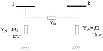
Figure 1. Model with variable resistance

2.png

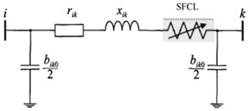
Figure 2. Equivalent diagram of a transmission line

where,

$\operatorname{Rsc}=\left\{\begin{array}{lr}o & (J<J c, T<T c) \\ \operatorname{Rc}\left(\frac{J}{J c}\right)^{n-1} & \text { if }(J>J c, T<T c) \\ \operatorname{Rsc} \max (T) & \quad(T>T c)\end{array}\right.$             (7)

Rsc: superconducting resistance, Rc: critical resistance of the superconductor,

Rsc max: Max superconducting resistance after the transition,

3.png

Figure 3. Model of SFCL inserted in the transmission line

4.png

Figure 4. Model of SFCL inserted in series with generator

The equivalent circuit in π of the transmission line with SFCL is illustrated in Figure 3. The following admittance matrix of the line can be formed [12]:

$Y_{i k}=\frac{1}{\left(r_{i k}+R_{S F C L}\right)+j x_{i k}}$                 (8)

where, r_ik, x_ik, and b_ikare resistance, reactance line, and capacitance line, respectively. R_SFCL is resistance of SFCL.

The equivalent circuit of generator equipped by SFCL is given by the figure 4.

When the resistive SFCL is placed in series with generator, the element of the admittance matrix is given by

$Y_{i k}=\frac{1}{\left(R_{G}+R_{S F C L}+J X_{d}^{1}\right)}$             (9)

where, $X_{d}^{1}$ is the d-axis generators transient reactance of generator, R_G is resistance of generator. R_SFCL are resistance of resistive SFCL, respectively.

So after inserting the SFCL into the network, there will be a significant change in the admittance matrix.

We present the simulation results obtained during a fault on a power grid with and without a current limiter using the PSIM software. The computation of Rsc max is done from the numerical code developed and implemented under the MATLAB environment, where we adopted the method of the finite volumes as method of resolution of the set of partial differential equations characteristic to the physical phenomena to be treated.

4.1 Spatial distribution of temperature t within the superconducting pellet (SFCL)

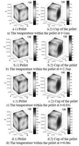
The results below represent the three-dimensional distribution of the temperature within the superconducting pellet used to limit the fault current. The temperature within the pellet increases gradually over time, which is to say with the increase of the fault current. The temperature reaches its maximum at the heart of the superconducting pellet and it decreases considerably on the walls of the pellet, this is due to the cooling effect of the cryogenic fluid.

6.png

Figure 6. Spatial distribution of the temperature within the pellet

When the current exceeds the critical current, the transition is initiated. The energy dissipated at the pellet heats the limiter constantly and homogeneously. If the pellet heats up to its critical temperature Tc, the material then passes by exceeding its critical temperature and goes into its normal state (transition from the superconducting state to the normal state).

7.png

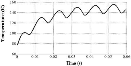
Figure 7. The variation of the temperature in the pellet as a function of time

Figure 6.a. Corresponds to the superconducting state of the pellet, the result has been noted at time t=1ms and in this case the limiter no longer intervenes. Because the maximum temperature inside the pellet is of the order of 79.8 ° K is lower than Tc.

Figure 6.b, c and d. Respectively recorded at times t=2.5 ms, t=0.03 s and t=0.06 s show how the limiter takes its normal state and comes into play limitation, the temperatures in the pellet are excessively of the order of 93.3 °K, 137.8 °K and 145.6 °K.

8.png

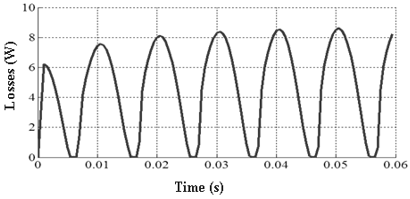
Figure 8. The variation of the average losses in the pellet as a function of time

Figure 7 Clearly shows the temporal evolution of the temperature within the superconducting pellet. It appears a beginning of transition at time t=2.5 ms, corresponds to a temperature close to the critical temperature.

Figure 8 illustrates the temporal evolution of the average losses in the pellet. These are increased over time because of the energy dissipated per unit volume within the superconducting pellet.

4.2 Inserting the SFCL into the network at nine- bus

4.2.1 Case of a two-phase fault

9.png

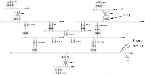
Figure 9. Nine-bus network with two-phase fault with SFCL

A short-circuit two-phase at the bus 8. PHASES terminals (V-W) is applied at time t=0.1s and for good visibility, the simulation is performed over a period of 0.4 s.

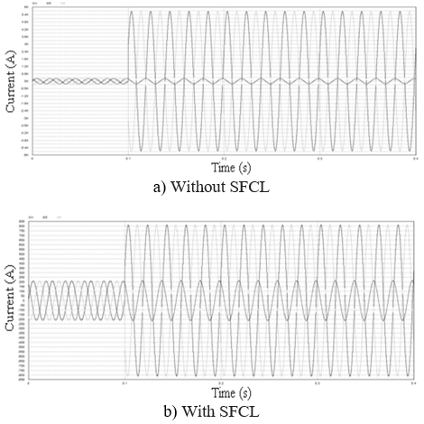
(1) Currents of the Line (4-7):

10.png

Figure 10. The pace of currents I1, I2, I3 of the line (4-7)

(2) Currents of the line (7-8):

11.png

Figure 11. The pace of the currents I4, I5, I6 of the line (7-8)

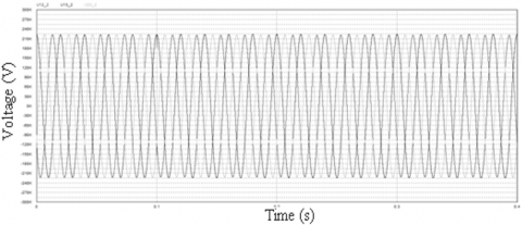
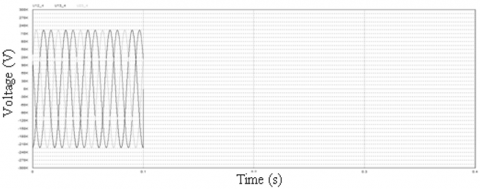
(3) Voltages of the line (7-8):

12.png

Figure 12. Waveform of the voltages U12, U23, U13 of the line (7-8) during two-phase fault

(4) Voltages of the line (4-7):

13.png

Figure 13. Waveform of the voltages U12, U23, U13 of the line (4-7) during two-phase fault

The Table 2 presents and collates the results of the currents recorded in the line (4-7) and in the line (7-8), also the transition time of SFCL.

Table 2. Two-phase short-circuit current values with and without SFCL limitation

4.2.2 Case of a three-phase fault

In this case, a short-circuit three-phase in the bus 8, phases terminals (U-V-W) is applied at time t=0.1s. The Table 3 presents and collates the results of the currents recorded in the line (4-7) and in the line (7-8), also the transition time of SFCL.

Table 3. Values of three-phase short-circuit currents with and without SFCL limitation

Figure 14 shows the voltages per phase of the line (7-8), whenever SFCL is placed in the power system network, precisely in bus 8.

14.png

Figure 14. Waveform of the voltages U12, U23, U13 of the line (7-8) during three-phase fault