Saad Khadar | Kouzou Abdellah | Hani Benguesmia
OPEN ACCESS
Five-phase fault-tolerant induction motor (FPIM) with open-end winding (OEW) can offer low torque ripple and it has a merit of high fault-tolerant capability due to its large number of phases. In order to improve the operation performance under an open single-phase. This paper proposes a Remedial Backstepping Control (RBSC) technique for a FPIM-OEW with the ability to run the system before and after fault condition. Hence, the FPIM-OEW losses are decreased, which improves the overall machine efficiency. The proposed RBSC technique lies in the orthogonal reduced-order transformation matrix, which is derived from the fault-tolerant current references, and a new zero-sequence current related to torque ripple. Also, the effect of the open-phase fault on the motor model under the transformation matrix is discussed. The simulation results of the proposed technique under open single-phase are provided, wherein we demonstrate the effectiveness of the proposed strategy with a fast dynamic and steady-state performances as that under healthy operation.
remedial backstepping control, open-phase fault, five-phase induction motor, transformation matrix, open end winding
In recent decades, multiphase machines have attracted more and more interest for their use in applications where high reliability such as in electric vehicles [1], aerospace [2], electric ship propulsion and wind power generation systems [3]. Current interest in these machines is mostly the consequence of their advantages, when compared to a power equivalent three-phase machines in terms of: reducing the amplitude and increasing the frequency of torque pulsation, reducing the current per phase without increasing the voltage per phase, and providing higher flux density and more output torque [4-6]. They have another distinguished advantage which is the improved reliability and continuous system operation even in the fault condition [7]. Among the available multiphase machines that have been proposed by Mengoni et al. and Immovilli et al. [8-10], the five-phase induction machines (FPIM) are now recognized as a practical selections in safety-critical high power applications, because of their ability to increase at least 10% of torque compared to its three-phase counterpart of the same active volume [11], in addition to the fact that they present a serious option that offers better machine performance under fault conditions [12].
On the other hand, multilevel inverters are used in single-sided supply mode for adjustable speed drive application. However, conventional multilevel inverters have some drawbacks such as dc link voltage balancing problems and the use of high rating capacitors [13]. Alternative solution for obtaining multilevel output is by supplying an open-end winding (OEW) machine using dual inverter [4]. The star point is opened and the supply is given from both sides of the motor through the inverters, which combines the advantages of high fault tolerance of multi-phase machines and high power quality of multilevel inverters and induction machines. This topology offers several advantages when compared with the traditional single-sided two-level inverter supplied motor [14, 15] such as higher redundancy, no clamping diodes or capacitors are needed and the possibility of the reduction of common mode voltage [4, 13]. However, an unexpected fault may occur due to improper operation. According to statistics from [16], among all types of faults, an open-phase or broken-phase of machines, short-circuiting of stator windings [17] and damage to switching devices in the five-phase bridge inverter are the most common. In FPIM with one phase open, when open-circuit fault occurs, a unbalanced currents are generated, which increases the induced torque ripple [18] and distorts the air gap flux distribution causing eventual motor breakdown [19]. In order to meet the requirement of high reliability applications, FPIM-OEW offers more degrees of freedom, which can be used with fault-tolerant control for compensation, thus ensuring the machine ability to continue to operate under fault conditions. Furthermore, many fault-tolerant control strategies for multiphase motors have been proposed in five [20], six [21], and seven phases [22], using permanent magnet synchronous motors and induction machines. A global fault-tolerance control technique is proposed by Mohammad and Parsa, and Scharlau et al. [23, 24], which can be applied to analyze all possible fault cases in any multi-phase motor regardless of the configuration of the motor’s stator windings.
Regarding the existing control techniques, the scalar control method (V/f) is simpler and still widely used in industrial fields. In the literature, the control of multiphase induction motor using V/f is addressed in healthy [25] and faulty operation [26]. The Rotor-Field Oriented Control (RFOC) method, based on PI controller loop, which requires accurate machine parameters, is the most widespread control technique in the multiphase case. This technique has been applied in FPIM in healthy [27] and faulty operation [28]. Another widely used control technique is the Direct torque control [29, 30]. Other well-known non-linear controller like Backstepping, has not been so deeply extended to the multiphase case, where only healthy operation of FPIM is considered [31]. Improving the fault-tolerant capability is a hot topic in FPIM [28, 18], [32-34]. However, this fault-tolerant capability using Backstepping methods has not been stated yet, being this a main contribution of our work. This paper proposes a Remedial BSC (RBSC) technique using a reduced-order transformation matrix for a FPIM-OEW. This strategy depends on choosing a Lyapunov function. The proposed orthogonal reduced-order transformation matrix can reduce the design complexity and can minimize torque ripple. Therefore, the proposed RBSC technique is conceptually clear and easy to realize.
This paper is organized as follows. Section 2 presents the FPIM-OEW detailed model. Section 3 presents the proposed RBSC technique with the transformation matrix is deduced. In Section 4, the simulation results will be given to verify the RBSC technique performance, before and after the fault event. The conclusions are finally summarized.
2.1 Modeling of five phase induction motor
This paper presents a FPIM with a squirrel-cage rotor and symmetrically distributed stator windings (with a fixed spatial displacement of $\alpha=\frac{2 \pi}{5}$ between windings), uniform air gap, and sinusoidal MMF distribution are considered [4]. The basic equations of FPIM under balanced condition are discussed in [35]. Defining γ=0.4π, the Clarke transformation matrix [19, 36], which transforms the phase variables into α-β and the zero-sequence subspace, and it will be referred to as TC can be written as:
$\left[T_{c}\right]=\frac{2}{5}\left[\begin{array}{ccccc}1 & \cos \gamma & \cos 2 \gamma & \cos 3 \gamma & \cos 4 \gamma \\ 0 & \sin \gamma & \sin 2 \gamma & \sin 3 \gamma & \sin 4 \gamma \\ 1 & \cos 3 \gamma & \cos 6 \gamma & \cos 9 \gamma & \cos 12 \gamma \\ 0 & \sin 3 \gamma & \sin 6 \gamma & \sin 9 \gamma & \sin 12 \gamma \\ 0.5 & 0.5 & 0.5 & 0.5 & 0.5\end{array}\right]$ (1)
The five phase stator currents of FPIM during healthy operation can be defined as following:
$\left\{\begin{array}{l}i_{s a}=i_{a 1}-i_{a 2} \\ i_{s b}=i_{b 1}-i_{b 2} \\ i_{s c}=i_{c 1}-i_{c 2} \\ i_{s d}=i_{d 1}-i_{d 2} \\ i_{s e}=i_{e 1}-i_{e 2}\end{array}\right.$ (2)
The total stator rotating magneto-motive forces (MMFs) is determined by the following formula:
$M M F=\sum_{A}^{E} M M F_{i}=N i_{s a}+a N i_{s b}+a^{2} N i_{s c}+a^{3} N i_{s d}+a^{4} N i_{s e}$ (3)
with: a=cosγ+jsinγ
The multiphase system modeling is usually simplified using the Vector Space Decomposition (VSD) approach [37]. For d-q-x-y reference, four independent variables divided in two orthogonal planes called d-q and x-y. However first components d-q are responsible for torque production, while x-y remaining components do not generate electrical torque and generates losses in the system [4]. An additional axis called z is also defined related to the zero-sequence component of the system. The dynamic equation of five phase induction motor in the d-q-x-y reference frame after transformation can be written in the following form [4]:
$\left\{\begin{array}{l}\frac{d i_{s d}}{d t}=\alpha_{1}+\frac{1}{\sigma L_{s}} V_{s d} \\ \frac{d i_{s q}}{d t}=\alpha_{2}+\frac{1}{\sigma L_{s}} V_{s q} \\ \frac{d i_{s x}}{d t}=\frac{R_{s}}{L l_{s}} i_{s x}+\frac{1}{L l_{s}} V_{s x} \\ \frac{d i_{s y}}{d t}=\frac{R_{s}}{L l_{s}} i_{s y}+\frac{1}{L l_{s}} V_{s y}\end{array}\right.$ (4)
$\left\{\begin{array}{l}\frac{d \psi_{r}}{d t}=\frac{L_{m}}{T_{r}} i_{s d}-\frac{\psi_{r}}{T_{r}} \\ \frac{d \omega}{d t}=\frac{n_{p}^{2} \psi_{r}}{J L_{r}}-\frac{n_{p}}{J} T_{L}-\frac{F}{J} \omega\end{array}\right.$ (5)
with:
$\alpha_{1}=-\frac{L_{m}^{2} R_{r}+R_{s} L_{r}^{2}}{\sigma L_{r}^{2} L_{s}} i_{d s}+\omega i_{s q}+\frac{L_{m} \psi_{r}}{\sigma L_{r} T_{r}}+\frac{L_{m} i_{s q}^{2}}{T_{r} \psi_{r}}$
$\alpha_{2}=-\frac{L_{m}^{2} R_{r}+R_{s} L_{r}^{2}}{\sigma L_{r}^{2} L_{s}} i_{s q}-\omega\left(i_{s q}+\frac{L_{m} \psi_{r}}{\sigma L_{r}^{2}}\right)-\frac{i_{s q} i_{s d} L_{m}}{T_{r} \psi_{r}}$
where: Rs, Rr, Lm, Ls and Lr are the stator resistance, the rotor resistance, the magnetizing inductance, the stator inductance and the rotor inductance, respectively. Lls=Ls-Lm is the stator leakage inductance, Llr=Lr-Lm is the rotor leakage inductance, np is the number of pole pairs.
2.2 Dual inverter open-end winding with one DC source
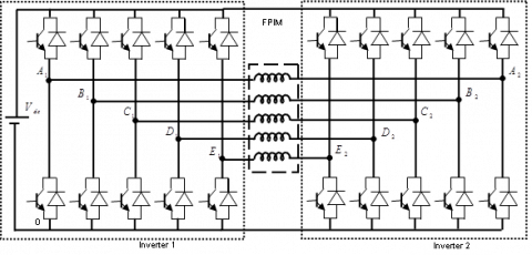
The proposed dual two-level inverter feeding the open-end stator winding of the five-phase induction motor is shown in Figure 1 [4], where only one DC source is used. The dual inverter are identified with indices 1 and 2. Inverter legs are denoted with capital letters A, B, C, D, E with their suffix 1 and 2, O is assumed virtual neutral point.
Figure 1. The dual five-phase voltage source inverter connected FPIM with one DC source
The phase voltages of the two inverters can be given as follows:
$\left\{\begin{array}{l}V_{s a}=V_{A 1}-V_{A 2} \\ V_{s b}=V_{B 1}-V_{B 2} \\ V_{s c}=V_{C 1}-V_{C 2} \\ V_{s d}=V_{D 1}-V_{D 2} \\ V_{s e}=V_{E 1}-V_{E 2}\end{array}\right.$ (6)
where, (VA1, VB1, VC1, VD1, VE1) are the five phase output voltages for inverter 1, (VA2, VB2, VC2, VD2, VE2) are the five phase output voltages for inverter 2.
3.1 Robust backstepping control based on field-oriented control
The basic idea of the Backstepping control (BSC) design is the use of the so-called virtual control to systematically decompose a complex nonlinear control design problem into simpler, smaller ones. BSC design is divided into various design steps [6, 38]. In each step we essentially deal with an easier, single-input-single-output design problem and each step will provide a reference for the next step. Stability and performance of our system will be studied using Lyapunov theory [4-6, 39]. The synthesis of this control can be achieved in two steps.
Step 1: Computation of the reference stator currents
Since the rotor speed and the rotor flux module are our control variables, we define the errors eω and eψ representing the error between the actual speed and the reference speed and the error between the rotor flux module and its reference, the tracking errors are defined by:
$\left\{\begin{array}{l}e_{\omega}=\omega^{*}-\omega \\ e_{\psi}=\psi_{r}^{*}-\psi_{r} \\ \dot{e}_{\omega}=\dot{\omega}^{*}-\dot{\hat{\omega}} \\ \dot{e}_{\psi}=\dot{\psi}_{r}^{*}-\dot{\psi}_{r}\end{array}\right.$ (7)
Accounting for Eq. (5), Eq. (7) turns to be:
$\left\{\begin{array}{l}e_{\omega}=\omega^{*}-\frac{n_{p}^{2} L_{m}}{J L_{r}} \hat{\psi}_{r} i_{s q}+\frac{F}{J} \omega+\frac{T_{L}}{J} n_{p} \\ \dot{e}_{\psi}=\dot{\psi}_{r}^{*}+\frac{\psi_{r}}{T_{r}}-\frac{L_{m}}{T_{r}} i_{s d}\end{array}\right.$ (8)
The first Lyapunov function associated with the speed and rotor flux errors can be defined as following:
$V_{1}=0.5\left(e_{\psi}^{2}+e_{\omega}^{2}\right)$
$\dot{V}_{1}=\left(-K_{\psi} \cdot e_{\psi}^{2}-K_{\omega} \cdot e_{\omega}^{2}\right)$ (9)
The pursuit of goals are achieved by choosing the references of the current components representing the stabilizing functions as [4]:
$\left\{\begin{array}{l}i_{s d}^{*}=\frac{T_{r}}{L_{m}}\left(K_{\psi} e_{\psi}+\dot{\psi}^{*}+\frac{\psi_{r}}{T_{r}}\right) \\ i_{s q}^{*}=\frac{L_{r}}{n_{p}^{2} L_{m} \psi_{r}}\left(\dot{\omega}^{*}+K_{o} e_{\omega}+\frac{F \omega}{J}+\frac{T_{L} n_{p}}{J}\right) \\ i_{s x}^{*}=0 \\ i_{s y}^{*}=0\end{array}\right.$ (10)
where, Kψ and Kψ are positive constants that determine the closed loop dynamics. To satisfy equation (10), we must choose the dynamic errors as the following form:
$\left\{\begin{array}{l}e_{\psi}=-K_{\psi} e_{\psi}^{2} \\ \dot{e}_{\omega}=-K_{\omega} e_{\omega}^{2}\end{array}\right.$ (11)
Thus, the tracking objectives will be satisfied if we choose. So, the control $i_{s d}^{*}$ and $i_{s q}^{*}$are asymptotically stabilizing and are considered as references for the next step.
Step 2: Computation of the reference stator voltages:
To calculate the control law $V_{s d}^{*}, V_{s q}^{*}, V_{s x}^{*}$ and $V_{s y}^{*}$ of the complete system, we will define in the second step the new errors $e_{i_{s d}}, e_{i_{s q}}, e_{i_{s x}}$ and $e_{i_{s y}}$, which represent respectively the errors signals between stator the current and their references as follows:
$\left\{\begin{array}{l}e_{i_{i d}}=i_{s d}^{*}-i_{s d} \\ e_{i_{i q}}=i_{s q}^{*}-i_{s q} \\ e_{i_{x}}=i_{s x}^{*}-i_{s x} \\ e_{i_{y}}=i_{s y}^{*}-i_{s y}\end{array}\right.$ (12)
The derivative of the stator current errors gives:
$\left\{\begin{array}{l}\dot{e}_{i_{z d}}=\dot{i}_{s d}^{*}-\dot{i}_{s d} \\ \dot{e}_{i_{g q}}=\dot{i}_{s q}^{*}-\dot{i}_{s q} \\ \dot{e}_{t_{x}}=\dot{i}_{s x}^{*}-\dot{i}_{s x} \\ \dot{e}_{i_{s}}=i_{s y}^{*}-i_{s y}\end{array}\right.$ (13)
Accounting for Eq. (6), Eq. (12) turns to be:
$\left\{\begin{array}{l}e_{i_{i d}}=\frac{d i_{s d}^{*}}{d t}-\alpha_{1}-\frac{1}{\sigma L_{r}} V_{s d} \\ \dot{e}_{i_{g}}=\frac{d i_{s q}^{*}}{d t}-\alpha_{2}-\frac{1}{\sigma L_{r}} V_{s q} \\ \dot{e}_{i_{\pi}}=\frac{d i_{s x}^{*}}{d t}-\frac{R_{s}}{L l_{s}} i_{s x}-\frac{1}{L l_{s}} V_{s x} \\ \dot{e}_{i_{y}}=\frac{d i_{s y}^{*}}{d t}-\frac{R_{s}}{L l_{s}} i_{s y}-\frac{1}{L l_{s}} V_{s y}\end{array}\right.$ (14)
The final Lyapunov function $V_{2}$ based on the errors of speed, rotor flux and of the stator currents, which is given by the following expression:
$V_{2}=\frac{1}{2}\left(e_{\psi}^{2}+e_{\omega}^{2}+e_{i_{sd}}^{2}+e_{i_{sq}}^{2}+e_{i_{sx}}^{2}+e_{i_{sy}}^{2}\right)$ (15)
By using (15), the derivative of the Lyapunov function is given by:
$\dot{V}_{2}=\left(e_{\psi} \dot{e}_{\psi}+e_{\omega} \dot{e}_{\omega}+e_{i_{s d}} \dot{e}_{i_{s d}}+e_{i_{s q}} \dot{e}_{i_{s q}}+e_{i_{s x}} \dot{e}_{i_{s x}}+e_{i_{s y}} \dot{e}_{i_{y}}\right)$ (16)
By replacing Eq. (14) in Eq. (16), one can obtain:
$\dot{V}_{2}=(-K_{\psi} e_{\psi}^{2}-K_{\omega} e_{\omega}^{2}-K_{i_{s d}} e_{i_{s d}}^{2}-K_{i_{s q}} e_{i_{s q}}^{2}-K_{i_{s x}} e_{i_{s x}}^{2}-K_{i_{s y}} e_{i_{s y}}^{2})+e_{i_{s d}}\left(\frac{L_{m}}{T_{r}} e_{\psi}+\frac{d i_{s d}^{*}}{d t}-\alpha_{1}\right.-\frac{V_{d s}}{\sigma L_{r}}+e_{i_{s d}} K_{i_{s d}}$
$+e_{i_{s g}}\left(\eta \psi_{r} e_{\omega}+\frac{d i_{s q}^{*}}{d t}-\alpha_{2}-\frac{V_{q s}}{\sigma L_{r}}+e_{i_{s q}} K_{i_{s q}}\right)+e_{i_{s x}}\left(\frac{d i_{s x}^{*}}{d t}-\frac{R_{s}}{L l_{s}} i_{s x}-\frac{1}{L l_{s}} V_{s x}+e_{i_{s x}} K_{i_{s x}}\right)$
$+e_{i_{s y}}\left(\frac{d i_{s y}^{*}}{d t}-\frac{R_{s}}{L l_{s}} i_{s y}\right.-\frac{1}{L l_{s}} V_{s y}+e_{i_{s y}} K_{i_{s y}}$ (17)
To ensure that the derivative of the Lyapunov function V2 must be negative:
$\dot{V}_{2}=\left\{\begin{array}{l}\left(-K_{\psi} e_{\psi}^{2}-K_{\omega} e_{\omega}^{2}-K_{i_{s d}} e_{i_{s d}}^{2}-K_{i_{s q}} e_{i_{s q}}^{2}-K_{i_{s r}} e_{i_{s r}}^{2}-K_{i_{s y}} e_{i_{s y}}^{2}\right)=0 \\ \left(\frac{L_{m}}{T_{r}} e_{\psi}+\frac{d i_{s d}^{*}}{d t}-\alpha_{1}-\frac{V_{s d}}{\sigma L_{r}}+e_{i_{s d}} K_{i_{s d}}\right)=0 \\ \left(\eta \psi_{r} e_{\omega}+\frac{d i_{s q}^{*}}{d t}-\alpha_{2}-\frac{V_{s q}}{\sigma L_{r}}+e_{i_{s q}} K_{i_{s q}}\right)=0 \\ \left(\frac{d i_{s x}^{*}}{d t}-\frac{R_{s}}{L l_{s}} i_{s x}-\frac{1}{L l_{s}} V_{s x}+e_{i_{s x}} K_{i_{s x}}\right)=0 \\ \left(\frac{d i_{s y}^{*}}{d t}-\frac{R_{s}}{L l_{s}} i_{s y}-\frac{1}{L l_{s}} V_{s y}+e_{i_{s y}} K_{i_{s y}}\right)=0\end{array}\right.$ (18)
The control voltages based on currents errors are given by:
$\left\{\begin{array}{l}V_{s d}^{*}=\sigma L_{s}\left(K_{s_{s d}} e_{i_{s d}}-\alpha_{1}+\frac{L_{m}}{T_{r}} e_{\psi}+d i_{s d}^{*} / d t\right) \\ V_{s q}^{*}=\sigma L_{s}\left(K_{i_{s q}} e_{i_{s q}}-\alpha_{2}+\eta \psi_{r} e_{\omega}+d i_{s q}^{*} / d t\right) \\ V_{s r}^{*}=\sigma\left(L l_{s}+L_{m}\right)\left(K_{i_{s x}} e_{i_{s x}}+d i_{s x}^{*} / d t-\frac{R_{s}}{L l_{s}} i_{s x}\right) \\ V_{s y}^{*}=\sigma\left(L l_{s}+L_{m}\right)\left(K_{i_{s y}} e_{i_{s y}}+d i_{s y}^{*} / d t-\frac{R_{s}}{L l_{s}} i_{s y}\right)\end{array}\right.$ (19)
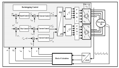
To ensure the control stability, the gains kisd,kisq,kisx and kisy should be considered positive by selecting the appropriate values. The block diagram of the proposed fault-tolerant RBSC for OEW-FPIM under single-phase open is shown in Figure 2.
Figure 2. The basic scheme for fault-tolerant Backstepping control of OEW-FPIM
3.2 Orthogonal reduced-order transformation matrices
The fault-tolerant capability of a motor means that the drive system can continue operation in satisfactory manner under fault condition [19]. Under open-circuit conditions, the currents in the remaining healthy phases can be continued, due to its independence of phases, we assume phase “A1-A2” as the open phase. As a consequence, the injected currents can be expressed as:
$i_{s a}=0$
$i_{s b}=1.382 \sin (w t-36)=-i_{s d}$
$i_{s c}=1.382 \sin (w t-144)=-i_{s e}$ (20)
For a FPIM-OEW with line ‘A1-A2’ assumed open, the remaining healthy phase currents that maintain the same rated fundamental MMF, thus providing the desired torque. The resultant MMF after the fault can be expressed as:
$M M F=\sum_{B}^{E} M M F_{i}=a N i_{s b}+a^{2} N i_{s c}+a^{3} N i_{s d}+a^{4} N i_{s e}$ (21)
It is worth noting that a disturbance-free operation can be achieved if the MMFs, produced by the phase windings, do not change in both healthy and fault conditions. Therefore, by using transformation, it can be derived as [40]:
For the healthy conditions
$\left[\begin{array}{l}i_{a s} \\ i_{b s} \\ i_{c s} \\ i_{d s} \\ i_{e s}\end{array}\right]=\left(\begin{array}{ll}1 & 0 \\ \cos \gamma & \sin \gamma \\ \cos 2 \gamma & \sin 2 \gamma \\ \cos 3 \gamma & \sin 3 \gamma \\ \cos 4 \gamma & \sin 4 \gamma\end{array}\right)\left(\begin{array}{cc}\cos \theta & -\sin \theta \\ \sin \theta & \cos \theta\end{array}\right)\left[\begin{array}{c}i_{s d}^{*} \\ i_{s q}^{*}\end{array}\right]$ (22)
For the fault conditions
$\left[\begin{array}{l}i_{b s} \\ i_{c s} \\ i_{d s} \\ i_{e s}\end{array}\right]=1.382\left(\begin{array}{ll}\cos 0.5 \gamma & \sin 0.5 \gamma \\ \cos 2 \gamma & \sin 2 \gamma \\ \cos 3 \gamma & \sin 3 \gamma \\ \cos 4.5 \gamma & \sin 4.5 \gamma\end{array}\right)\left(\begin{array}{cc}\cos \theta & -\sin \theta \\ \sin \theta & \cos \theta\end{array}\right)\left[\begin{array}{c}i_{s d}^{*} \\ i_{s q}^{*}\end{array}\right]$ (23)
It can be noted from (22) and (23) that the amplitudes of the healthy phase currents enlarge to 1.382 times at fault-tolerant operation, and the phasors of C1-C2 phase and D1-D2 phase remain their original places. Meanwhile, the phasor angles of B1-B2 phase and E1-E2 phase shift 0.2π, and A1-A2 phase phasor disappears. Hence, the current phasors under fault-tolerant condition are different from that under healthy condition. The use of the normal decoupling transformation matrices results in coupling currents [41]. Therefore, in order to perform BSC in the fault-tolerant operation, the transformation matrices have to be redefined. The production of the transformation matrix and its inverse matrix should be an identity matrix, the orthogonal reduced order transformation matrix can be derived as:
$[\Gamma]=\left[\begin{array}{cccc}\frac{\cos 0.5 \gamma}{3.618} & \frac{\cos 2 \gamma}{3.618} & \frac{\cos 3 \gamma}{3.618} & \frac{\cos 4.5 \gamma}{3.618} \\ \frac{\sin 0.5 \gamma}{1.91} & \frac{\sin 2 \gamma}{1.91} & \frac{\sin 3 \gamma}{1.91} & \frac{\sin 4.5 \gamma}{1.91} \\ \frac{\sin \gamma}{5} & \frac{\sin 4 \gamma}{5} & \frac{\sin 6 \gamma}{5} & \frac{\sin 9 \gamma}{5} \\ 1 & 1 & 1 & 1\end{array}\right]$ (24)
The inverse transformation matrix is:
$[\Gamma]^{-1}=1.382\left[\begin{array}{cccc}\cos 0.5 \gamma & \sin 0.5 \gamma & \sin \gamma & 0.181 \\ \cos 2 \gamma & \sin 2 \gamma & \sin 4 \gamma & 0.181 \\ \cos 3 \gamma & \sin 3 \gamma & \sin 6 \gamma & 0.181 \\ \cos 4.5 \gamma & \sin 4.5 \gamma & \sin 9 \gamma & 0.81\end{array}\right]$ (25)
To introduce the BSC strategy into fault-tolerant operation, the FPIM model should be rewritten under phase (A1-A2) open-circuit fault:
$\left\{\begin{array}{l}V_{sfd}=i_{s f d} R_{s}+L_{s} \frac{d i_{s f d}}{d t}-\omega L_{s} i_{s f q} \\ V_{sfq}=i_{s f q} R_{s}+L_{s} \frac{d i_{s f q}}{d t}+\omega L_{s} i_{s f d} \\ V_{z}=i_{z} R_{s}+L l_{s} \frac{d i_{z}}{d t} \\ V_{0}=0\end{array}\right.$ (26)
By applying (23), the voltage references can be obtained as:
$\left[\begin{array}{c}V_{b s} \\ V_{c s} \\ V_{d s} \\ V_{e s}\end{array}\right]=\Gamma^{-1} \Pi^{-1}\left[\begin{array}{c}V_{s f d} \\ V_{s f q} \\ V_{z} \\ V_{0}\end{array}\right]+\left[\begin{array}{c}e_{b} \\ e_{c} \\ e_{d} \\ e_{e}\end{array}\right]$ (27)
where:
$\left[\begin{array}{l}e_{b} \\ e_{c} \\ e_{d} \\ e_{e}\end{array}\right]=-\omega \psi_{r}\left[\begin{array}{l}\sin (\theta-0.5 \gamma) \\ \sin (\theta-2 \gamma) \\ \sin (\theta-3 \gamma) \\ \sin (\theta-4.5 \gamma)\end{array}\right]$ (28)
The proposed RBSC technique is different from the previous published works [3, 22, 34, 42], in which the reduced order transformation matrix of the post-fault have been identified. The proposed strategy simplifies the matching design of the transformation matrix. Also, it needs no solution to the generalized zero-sequence current, thus the fault-tolerant RBSC technique can be easily realized.
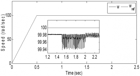
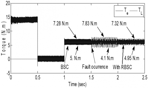
In this section, to prove the viability the efficiency of the proposed RBSC scheme, the Matlab/ Simulink software package has been used for the purpose of testing the motor under healthy as well as open phase cases. The parameters of the studied OEW-FPIM for simulation are listed in the following: Rs=10Ω, Rr=6.3Ω Ls=0.4642H, Lr=0.4642H, Msr=0.4212H, J=0.02 Kg⁄m2, F=0N.m.s The reference rotor flux used is 1 Wb. The performed test considers that the open-phase fault condition occurs in phase ‘A1-A2’ and the fault occurrence is emulated by opening a power relay connected in series with the faulty phase. When open-circuit fault occurs in phase (A1-A2), the Park transformation matrix and their inverse matrices are replaced by (22), (23) and their inverse matrices. It is assumed that a step reference speed of 100 rad/s is applied with the machine mechanically unloaded and then it is loaded with its load torque of 7 N.m at 1s. The resulting waveforms for RBSC are shown in Figure 3 to Figure 7, side by side, speeds, torque, d-q rotor flux, d-q stator current and flux trajectory are recorded. During the BSC method of the FPIM-OEW drive, the phase open-circuit fault occurs at 1 s, and then the RBSC method is activated at 2s. The reference and real speed are shown in Figure 3. The fault occurs at time t=1.5 s, it is observed that the real speed has more vibration suggesting that the loss of phase “A1-A2” cause more serious asymmetry for the motor. After one second. The motor speed ripple are decreased, when the proposed RBSC algorithm is applied, as it is illustrated in Figure 3.
Figure 3. The reference and real speed
Figure 4. The electromagnetic torque
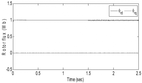
Figure 5. The d-q rotor flux
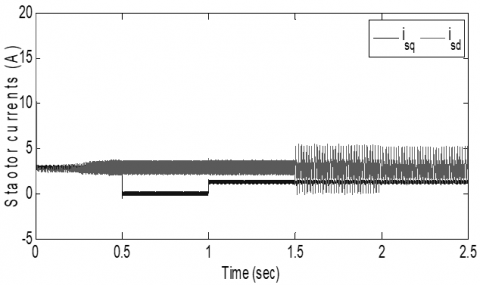
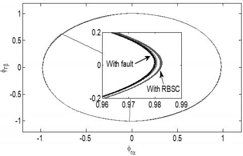
The load torque and the developed electromagnetic torque by the studied motor are shown in Figure 4. As a result of the improper control, the remaining phase currents are distorted, thus resulting in significant torque oscillation (3.73 N.m). When the RBSC is activated, it is also observed that the proposed controller reduces the torque oscillation considerably (2.37 N.m). Therefore, the proposed RBSC can retain the steady-state torque performance as the healthy operation (2.28 Nm), ensuring high performance for torque control under single-phase open. According to Figure 6 which presents the d-q-axis stator current response, before and after the fault appearance. It can be seen that isd is constant, while isq is approximately proportional to the electromagnetic torque. Therefore, in fault condition, the frequency of the torque fluctuation is the same as that of the q-axis current fluctuation, as illustrated in Figure 6. The performance of the trajectory of the α-β rotor flux is also shown in Figure 7. In fault condition, due to d-axis stator current disruption, the trajectory of the rotor flux is elliptical. When the RBSC is activated, the trajectory of the rotor flux with RBSC is circular, which coincides with that under healthy condition.
Figure 6. The d-q stator currents of OEW-FPIM
Figure 7. The trajectory of the α-β rotor flux
According to the elaborated results. It can be seen that the transition from the pre-fault to the post-fault situation is almost unnoticeable. So, the RBSC strategy is effective during the loss of one phase, offering a similar performance as in healthy condition.
The single-phase open fault being the most common type of faults, it is next analyzed in a generic multiphase machine with an odd number of phases. This paper has proposed a RBSC strategy for the FPIM-OEW with single-phase open. Its unique contribution is the derived orthogonal reduced-order transformation matrix. Firstly, the effect of an open-phase fault condition has been modeled, showing that it is necessary to modify the transformation matrix. Next, a phase domain motor model has been presented, which has the ability to provide insight into the behaviour of a FPIM-OEW after loss of phase. The transformation matrix has been derived from the optimal fault-tolerant currents. Finally, the simulation results conclude that the proposed control technique can operate the machine after the fault occurrence using the healthy phases. Also, the compensation strategy ensures disturbance-free operation, and has the same dynamic and steady-state performances as that under healthy operation. Additionally, the RBSC strategy requires no extra hardware, except the transformation matrices. Therefore, the proposed RBSC strategy is simple and easy to be implemented.
Acronyms
RBSC: Remedial Backstepping Control
BSC: Backstepping Control
FPIM: Five phase induction motor
OEW: Open-end winding
FPIM-OEW: Five phase induction motor open-end winding
RFOC: Rotor-Field Oriented Control
MMFs: Magnetomotive forces
VSD: Vector Space Decomposition
[1] Riveros, J., Bogado, B., Prieto, J., Barrero, F., Toral, S., Jones, M. (2010). Multiphase machines in propulsion drives of electric vehicles. In Proceedings of 14th International Power Electronics and Motion Control Conference EPE-PEMC 2010, T5-201. https://doi.org/10.1109/EPEPEMC.2010.5606658
[2] de Lillo, L., Empringham, L., Wheeler, P.W., Khwan-On, S., Gerada, C., Othman, M.N., Huang, X. (2010). Multiphase power converter drive for fault-tolerant machine development in aerospace applications. IEEE Transactions on Industrial Electronics, 57(2): 575-583. https://doi.org/10.1109/TIE.2009.2036026
[3] Duran, M., Barrero, F. (2016). Recent Advances in the Design, Modeling and Control of Multiphase Machines – Part 2. IEEE Transactions on Industrial Electronics, 63(1): 459-468. https://doi.org/10.1109/TIE.2015.2448211
[4] Khadar, S., Kouzou, A., Hafaifa, A., Iqbal, A. (2019). Investigation on SVM-Backstepping sensorless control of five-phase open-end winding induction motor based on model reference adaptive system and parameter estimation. Engineering Science and Technology, an International Journal, https://doi.org/10.1016/j.jestch.2019.02.008, 2019
[5] Layadi, N., Zeghlache, S., Benslimane, T., Berrabah, F. (2017). Comparative Analysis between the Rotor Flux Oriented Control and Backstepping Control of a Double Star Induction Machine (DSIM) under Open-Phase Fault. AMSE Journals, Series Advances C, 72(4): 292-311.
[6] Rahali, H., Zeghlache, S., Benalia, L., Layadi, N. (2007). Sliding mode control based on backstepping approach for a double star induction motor (DSIM). Advances in Modelling and Analysis, 73(4): 150-157.
[7] Ryu, H.M., Kim, J.W., Sul, S.K. (2006). Synchronous frame current control of multiphase synchronous motor under asymmetric fault condition due to open phases. IEEE Trans. on Ind. Appl., 42(4): 1062-1070.
[8] Mengoni, M., Zarri, L., Tani, A., Parsa, L., Serra, G., Casadei, D. (2015). High-torque density control of multiphase induction motor drives operating over a wide speed range. IEEE Transactions on Industrial Electronics, 62(2): 814-825. https://doi.org/10.1109/TIE.2014.2334662
[9] Mengoni, M., Zarri, L., Tani, A., Gritli, Y., Serra, G., Filippetti, F., Casadei, D. (2015). On-line detection of high-resistance connections in multiphase induction machines. IEEE Trans. Power Electron, 30(8): 4505-4513.
[10] Immovilli, F., Bianchini, C., Lorenzani, E., Bellini, A., Fornasiero, E. (2015). Evaluation of combined reference frame transformation for inter-turn fault detection in permanent magnet multi-phase machines. IEEE Trans. on Ind. Electron, 62(3): 1912-1920. https://doi.org/10.1109/TIE.2014.2348945
[11] Toliyat, H.A., Lipo, T.A., White, J.C. (1991). Analysis of a Concentrated Winding Induction Machine for Adjustable Speed Drive Applications Part II: Motor Design and Performance. IEEE Trans. on Energy Convers, 6(4): 684-692. https://doi.org/10.1109/60.103642
[12] Levi, E. (2008). Multiphase electric machines for variable-speed applications. IEEE Transactions on Energy Conversion, 55(5): 1893-1909.
[13] Khadar, S., Kouzou, A. (2018). Implementation of Control Strategy Based on SVM for Open-End Winding Induction Motor with short circuit fault between turns in Stator Windings. Journal of Automation & Systems Engineering, 12(3): 12-25.
[14] Kim, J., Jung, J., Nam, K. (2004). Dual-inverter control strategy for high speed operation of EV induction motors. IEEE Trans. on Ind. Electron, 51(2): 312-320. https://doi.org/10.1109/TIE.2004.825232
[15] Kawabata, Y., Nasu, M., Nomoto, T., Ejiogu, E.C., Kawabata, T. (2002). High efficiency and low acoustic noise drive system using open winding AC motor and two space-vector-modulated inverters. IEEE Trans. on Ind. Electron, 49(4): 783-789.
[16] Cheng, M., Hang, J., Zhang, J. (2015). Overview of fault diagnosis theory and method for permanent magnet machine. Chinese Journal of Electrical Engineering, 1(1): 21-36. https://doi.org/10.23919/CJEE.2015.7933135
[17] Bechkaoui, A., Ameur, A., Bouras, S., Ouamrane, K. (2014). Diagnosis of Turn Short Circuit Fault in PMSM Sliding-mode Control based on Adaptive Fuzzy Logic-2 Speed Controller. AMSE Journals, 70(1): 29-45.
[18] Abdel-Khalik, A., Ahmed, S., Elserougi, A., Massoud, A. (2015). Effect of stator winding connection of five-phase induction machines on torque ripples under open line condition. IEEE/ASME Trans. Mechatronics, 20(2): 580-593.
[19] Zhou, H., Zhao, W., Liu, G., Cheng, R., Xie, Y. (2016). Remedial field-oriented control of five-phase fault-tolerant permanent-magnet motor by using reduced-order transformation matrices. IEEE Transactions on Industrial Electronics, 64(1), 169-178. https://doi.org/10.1109/TIE.2016.2599501
[20] Dwari, S., Parsa, L. (2008). Fault–Tolerant Control of Five-Phase Permanent-Magnet Motors with Trapezoidal Back EMF. IEEE Trans. on Ind. Electron, vol. 58, no. 2, pp. 476-485. 2011. Phase. IEEE Trans. on Ind. Electron, 55(5): 1966-1977.
[21] Locment, F., Semail, E., Kestelyn, X. (2008). Vectorial approach-based control of a seven-phase axial flux machine designed for fault operation. IEEE Trans. on Ind. Electron, 55(10): 3682-3691.
[22] Mohammad, A., Parsa, L. (2015). Global Fault-Tolerant Control Technique for Multi-Phase Permanent-Magnet Machines. IEEE Transactions on Industry Applications, 51(1): 178-186. https://doi.org/10.1109/TIA.2014.2326084
[23] Mohammad, A., Parsa, L. (2013). A unified fault-tolerant current control approach for five-phase PM motors with trapezoidal back EMF under different stator winding connections. IEEE Transactions on Power Electronics, 28(7): 3517-3527.
[24] Scharlau, C., Pereira, L., Haffner, S. (2008). Performance of a fivephase induction machine with optimized air gap field under open loop V/f control. IEEE Trans. on Energy Convers, 23(4): 1046-1056. https://doi.org/10.1109/TEC.2008.2001437
[25] Morsy, A., Abdel-khalik, A.S., Abbas, A., Ahmed, S., Massoud, A. (2013). Open loop V/f control of multiphase induction machine under open circuit phase faults. Twenty-Eighth Annual IEEE Applied Power Electronics Conference and Exposition, APEC'2013, Long Beach, CA, USA, 17-21 March 2013, Proc. 1170-1176.
[26] Lim, C.S., Levi, E., Jones, M., Rahim, N.A., Hew, W.P. (2014). FCS-MPC Based Current Control of a Five-Phase Induction Motor and its Comparison with PI-PWM Control. IEEE Transactions on Industrial Electronics, 61(1): 149-163. https://doi.org/10.1109/TIE.2013.2248334
[27] Guzman, H., Duran, M.J., Barrero, F., Bogado, B., Toral, S. (2014). Speed Control of Five-Phase Induction Motors with Integrated Open-Phase Fault Operation Using Model-Based Predictive Current Control Techniques. IEEE Trans. on Ind. Electron, 61(9): 4474-4484. https://doi.org/10.1109/TIE.2013.2289882
[28] Zheng, L., Fletcher, J.E., Williams, B.W., He, X. (2011). A Novel Direct Torque Control Scheme for a Sensorless Five-Phase Induction Motor Drive. IEEE Trans. on Ind. Electron, 58(2): 503-513. https://doi.org/10.1109/TIE.2010.2047830
[29] Bermudez, M., Gonzalez-Prieto, I., Barrero, F., Duran, M.J., Kestelyn, X. (2016). Open-Phase Fault Operation of 5-Phase Induction Motor Drives using DTC Techniques. 41st Annual Conference of the IEEE Industrial Electronics Society, IECON'2015, Yokohama, Japan, 9-12 Nov. 2015, Proc. IEEE, 2016.
[30] Echeikh, H., Trabelsi, R., Iqbal, A., Bianchi, N., Mimouni, M.F. (2016). Non-linear backstepping control of five-phase IM drive at low speed conditions-experimental implementation. ISA Trans, 65: 244-253. https://doi.org/10.1016/j.isatra.2016.06.013
[31] Abdel-Khalik, A.S., Elgenedy, M.A., Ahmed, S., Massoud, A.M. (2016). An Improved Fault-Tolerant Five-Phase Induction Machine Using a Combined Star/Pentagon Single Layer Stator Winding Connection. IEEE Trans. on Ind. Electron, 63(1): 618-628. https://doi.org/10.1109/TIE.2015.2426672
[32] Guzman, H., Duran, M.J., Barrero, F., Zarri, L., Bogado, B., Gonzalez-Prieto, I., Arahal, M.R. (2016). Comparative Study of Predictive and Resonant Controllers in Fault-Tolerant Five-phase Induction Motor Drives. IEEE Trans. on Ind. Electron, 63(1): 606-617. https://doi.org/10.1109/TIE.2015.2418732
[33] Tani, A., Mengoni, M., Zarri, L., Serra, G., Casadei, D. (2012). Control of Multiphase Induction Motors with an Odd Number of Phases Under Open-Circuit Phase Faults. IEEE Trans. Power Electron, 27(2): 565-577. https://doi.org/10.1109/TPEL.2011.2140334
[34] Libo, Z., Fletcher, J.E., Williams, B.W. (2008). Dualplane vector control of a five-phase induction machine for an improved flux pattern. IEEE Trans. on Ind. Electron, 55(5): 1996-2005. https://doi.org/10.1109/TIE.2008.918464
[35] Liu, G., Qu, L., Zhao, W., Chen, Q., Xie, Y. (2016). Comparison of two SVPWM control strategies of five phase fault-tolerant permanent-magnet motor. IEEE Trans. on Power Electron, 31(9): 6621-6630. https://doi.org/10.1109/TPEL.2015.2499211
[36] Levi, E., Bojoi, R., Profumo, F., Toliyat, H., Williamson, S. (2007). Multiphase induction motor drives-A technology status review. IET Elect. Power Appl, 1(4): 489-516. https://doi.org/10.1049/iet-epa:20060342
[37] Moutchou, M., Abbou, A., Mahmoudi, H. (2015). MRAS-based sensorless speed backstepping control for induction machine, using a flux sliding mode observer. Turkish Journal of Electrical Engineering and Computer Sciences, 23: 187-200.
[38] Jagannathan, S., Lewis, F.L. (2000). Robust backstepping control of a class of nonlinear systems using fuzzy logic. Information Sciences, 123(3): 223-240. https://doi.org/10.1016/S0020-0255(99)00128-0
[39] Liu, G., Qu, L., Zhao, W., Chen, Q., Xie, Y. (2016). Comparison of two SVPWM control strategies of five phase fault-tolerant permanent-magnet motor. IEEE Trans. on Power Electron, 31(9): 6621-6630. https://doi.org/10.1109/TPEL.2015.2499211
[40] Duran, M.J., Barrero, F. (2016). Recent advances in the design, modeling, and control of multiphase machines -part II. IEEE Trans. Ind. Electron, 63(1): 456-468. https://doi.org/10.1109/TIE.2015.2448211
[41] Che, H.S., Duran, M.J., Levi, E., Jones, M., Hew, W.P., Abd Rahim, N. (2014). Post-fault operation of an asymmetrical six-phase induction machine with single and two isolated neutral points. IEEE Trans. Power Electron, 29(10): 5406-5416. https://doi.org/10.1109/TPEL.2013.2293195