Soufiane Guedda | Djilani Benattous | Oussama Belaroussi* | Yacine Labbi | Ilyes Chaouki | Djaafer Toumi | Misbah Al-Awamer
© 2026 The authors. This article is published by IIETA and is licensed under the CC BY 4.0 license (http://creativecommons.org/licenses/by/4.0/).
OPEN ACCESS
Real-time observation of power systems is highly required for security and reliability purposes. Phasor Measurement Units (PMU) provide real-time and accurate measurement of voltage and current phasors. Nevertheless, the Optimal Phasor Measurement Units Placement (OPP) is demanded due to the high costs associated with the placement and communication infrastructures of PMUs. This paper presents a comprehensive, reproducible, and dependable comparative study of four different families of algorithms, representing four different algorithmic paradigms, to solve the OPP problem under a uniform model of topological observability. The studied algorithms encompass Depth-First Search (DFS)-based heuristics, Graph-Theoretic approach (GTh), a Modified Simulated Annealing (M-SA) metaheuristic algorithm, and a Recursive N-Security (RSN) algorithm. All the studied algorithms were implemented in MATLAB and tested on the well-known IEEE 14-, 30-, 57-, 118-bus systems in addition to the New England 39-bus system. The experimental results show that the RSN-based algorithm achieves the least number of PMUs needed for complete observability in most of the test bus systems. On the contrary, the proposed M-SA algorithm mainly shows faster execution time, especially for bus systems with high connectivity, while RSN is faster in poorly connected large bus systems. In summary, no single algorithm paradigm is more successful than the others at all benchmarks. The choice of the algorithm paradigm should be made based on the specific network topology and the desired trade-off between the minimization of the placement cost and the speed of execution in the case of contingency observation.
Phasor Measurement Units, power system observability, Optimal Phasor Measurement Units Placement, Depth-First Search, Simulated Annealing, Recursive N-Security Algorithm, Graph-Theoretic procedure
Today's electric power systems, with all the complexity and interdependence created by renewable-energy sources, need real-time monitoring and secure operation more than ever. These systems are centrally monitored from a control center where the operator deploys advanced visualization and diagnostic tools to maintain the stability, security and overall reliability of the network in normal and emergency situations [1-3]. The tool that provides this visibility is state estimation, which allows deriving, on a continuous basis, the most probable operational states of the system based on the information collected from the field at the substations [4, 5].
Accuracy of the state estimation process heavily depends on the nature of the measurement scheme, particularly number, type and location of the measurement devices [6, 7]. Many algebraic approaches scrutinize the measurement Jacobian rank to assess state uniqueness; however, performing numerical rank tests can become problematic due to ill-conditioning encountered in large systems running on tight tolerances [8-11]. The topological observability, in contrast, employs the properties of graph theory to establish the measurable areas using a previously defined spanning tree, thus eliminating the need to work with the complicated numerical state-estimation equations [12, 13]. In the topological framework, the Optimal Phasor Measurement Units Placement (OPP) problem is posed to make the whole network observable by using minimum number of devices or enhance its redundancies while abiding by the strict budgetary barriers [14, 15]. The PMUs’ time-synchronized high-rate dynamic measurements allow real-time views of the grid’s transient behavior [16-19].
To tackle the problem of optimal placement of Phasor Measurement Units (PMUs), advances in ILP/MILP, contingency-aware placement, zero-injection-bus (ZIB) modelling, and exceptional metaheuristic optimization continue to emerge. New comprehensive reviews and mathematical formulations have shown the incorporation of degree centrality with ILP for increasing effective observation of the transmission network [20, 21]. Recently developed nature- and epidemic-inspired metaheuristics, like coronavirus herd-immunity optimizer [22], and quasi-oppositional artificial-rabbit optimization [23], have been found effective to minimize the PMU placement cost while controlling wide-area monitoring data traffic [24-27].
The contributions for this paper, unlike the contemporary works that present a novel optimizer, precludes the design of a new optimizer:
2.1 Mathematical formulation
The proposed OPP problem focuses on optimizing the determination of the least number of PMUs capable of full observability for an N-bus power system. The measurement model of PMUs can be linearized as follows:
$z=h(x)+e$ (1)
where, z is the measurement vector and x is the state vector. For a system with N buses, a system is said to be numerically observable if.
$\operatorname{Rank}(h)=2 N-1$ (2)
The placement decision is modelled using a binary decision variable for each bus i: xi = 1 if a PMU is installed at bus i; xi = 0 otherwise.
The objective function minimizes the total number of installed PMUs:
$\min \sum_{i=1}^{N_{\text {bus }}} X_i$ (3)
This minimization has the topological observability limitation that each bus must be topologically observed at least once. The direct observability constraint is described by using the network binary connectivity matrix A — where Ai,j = 1 if buses i and j are connected and Ai,j = 1 — the direct observability constraint is expressed as:
$f(X)=A \cdot X \geq I$ (4)
where, X = [x1, x2, …, xN]T is the vector of decision variables and I is an N-dimensional vector of ones. Each row of the inequality guarantees that bus i is observed by a PMU placed either at itself or at one of its neighbors.
2.2 Topological observability rules
Topology-based observability allows for the reconstruction of system states from measurements through three essential network rules.
Rule 1: PMU at bus will directly measure voltage phasor of the concerned bus and current phasors of all branches associated with that bus (Figure 1).
Figure 1. Phasor Measurement Units (PMU) placement Rule 1: observability with direct measurements
Rule 2: The pseudo-measured data must ensure that the bus voltage is always observable. The placement of PMU according to Rule 2 is shown in Figure 2.
Figure 2. Phasor Measurement Units (PMU) placement Rule 2: observability of bus voltage using pseudo-measurements
Rule 3: PMU Placement - Pseudo-measurements to observe branch current. As shown in Figure 3, if branches have only one terminal in the grid with some load, node current injection can be constructed. If the branch has both terminals present in the gird bus, then branch current can be directly calculated through PMU measurements and used to determine current at other end of branch too.
Figure 3. Phasor Measurement Units (PMU) placement Rule 3: observability of branch current using pseudo-measurements
2.3 Zero-injection bus modeling
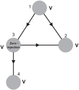
ZIB are those buses that do not generate or consume any active power. ZI buses also contribute to observability, without installing any PMU equipment at the ZIB. Kirchhoff’s Current Law (KCL) and Voltage Law (KVL) can be formulated around the ZI bus, and if only one of the adjacent nodes is not observable, the nodal variables can be found from a simple algebraic operation (Figure 4). In the case of adjacent ZI buses, if both adjacent buses have an unknown voltage phasor, we can write KCL and KVL equations considering the set of nodes referred to by that set of adjacent ZI buses: unknowns can be solved for both cases (Figures 5 and 6). In the constraint A · X ≥ I, this phenomenon is reflected by relaxing the observability of the ZI bus and its adjacent node but, in variating the number of unknowns found in a ZI bus’s adjacency, one of the number of unknowns found in the ZI group of buses can be solved based on these pseudo-measurements, rather than solving it from a direct PMU coverage.
Figure 4. Observability of a zero-injection bus (ZIB) using Kirchhoff’s Current Law (KCL) equations
Figure 5. Observability of an adjacent zero-injection bus (ZIB) with unknown voltage phasor
Figure 6. Observability of adjacent zero-injection buses (ZIB) with unknown voltage phasors
In this research, four different algorithms are used to solve the OPP defined above. To ensure impartiality, all algorithms are solved under the same observability rules used in Section 2, and the same connectivity-matrix observability criteria.
3.1 Depth-First Search heuristic
In this context, Depth-First Search (DFS) is used as a graph-search placement heuristic rather than a pathfinding algorithm. The algorithm will start with the bus with the highest degree and traverse the network in depth-first manner, while maintaining a stack of the unobserved buses. Upon reaching a high-degree node where at least one of its neighboring buses is unobserved, a PMU is placed at that location and Rules 1 to 3 are executed to mark the newly observed buses as observed. The algorithm continues traversing down the branches until all buses are marked as observed. The objective function in this case is the number of PMUs placed, observability is checked after each placement using A · X ≥ I and the algorithm halts when every bus has been shown observable. Due to this greedy and localized decision making, DFS is fast to complete although it does return a larger-than-necessary number of PMUs. The algorithm is summarized in Figure 7.
Figure 7. Modified Depth-First Search (DFS) flowchart for Phasor Measurement Units (PMU) placement
3.2 Graph-Theoretic procedure
The Graph-Theoretic-based method works directly on the adjacency matrix. It builds a minimal spanning tree for the grid, that already embeds the prioritization of ZI buses and the ability to optimally cut radial branches during its process. The Graph-Theoretic approach (GTh) method achieves a more globally-aware placement (i) by clustering the ZI clusters, and (ii) by maximizing their branch interconnections. The method is presented with a single consistent label throughout the paper (“GTh / Graph-Theoretic procedure”). The terminology “Greedy-Threshold” used before has been replaced to avoid confusion. The functionality of the method presented here was a Graph-Theoretic spanning-tree procedure, as further detailed in Figure 8.
Figure 8. Graph-Theoretic (GTh) method for Optimal Phasor Measurement Units Placement (OPP)
3.3 Original and Modified Simulated Annealing (O-SA / M-SA)
The original simulated annealing (O-SA) searches for candidate placement vectors and is allowed to probabilistically accept worse candidates, based on its cooling-temperature schedule, to break out of local optima. The O-SA searches a neighboring solution starting from an initial placement vector , x0, and parameters (T, k, c); A worse candidate is accepted with probability exp(−Δf / kT); where Δf refers to the difference of objective function, r is a uniformly distributed random number, r ∈ (0,1), and the temperature is reduced geometrically by factor c as T ← c · T until the stopping criterion is reached (Figure 9). The Modified Simulated Annealing (M-SA) retains the acceptance criteria, but applies different neighbor searcher: M-SA performs more robust, multi-bus candidate perturbations than mere single-bus swaps. Moreover, when identification of candidate stagnation occurs (no improvements for a set number of consecutive calls), M-SA applies candidates of even more severe structural perturbation with simultaneous relocation of a block of PMUs. The more aggressive candidate generation allows for a faster convergence to potentially more optimal solutions over the non-linear topologies defining larger grids. Both parametric settings for either variant are delivered in Table 1.
Figure 9. Methodological flowchart of the Simulated Annealing optimization algorithm
Table 1. Parameter settings of the original simulated annealing (O-SA) and Modified Simulated Annealing (M-SA) algorithms
|
Parameter |
Symbol |
Role |
Value |
|
Initial solution vector |
x0 |
Starting PMU placement vector |
random feasible |
|
Initial temperature |
T0 |
Controls early acceptance of worse solutions |
100 |
|
Cooling rate |
c |
Geometric cooling factor, T ← c · T |
0.95 |
|
Boltzmann scaling |
k |
Scales the acceptance probability |
1 |
|
Acceptance rule |
— |
Accept worse solution if r < exp(−Δf / kT), r ∈ (0,1) |
— |
|
Inner-loop length |
L |
Iterations evaluated at each temperature level |
100 |
|
Termination |
— |
Max iterations reached or temperature floor |
T ≤ 1 × 10⁻³ |
|
M-SA perturbation |
— |
Multi-bus disruptive mutation triggered on stagnation (vs. single-bus swap in O-SA) |
3-bus block |
3.4 Recursive N-Security algorithm
RSN best placed candidate is a greedy path search-based set-covering algorithm for minimum number of devices. Starting from topological bus with a high priority, the algorithm picks recursively the placement that provides maximum coverage to unobserved parts of the network. At every iteration, it checks if there are unobservable buses available; if so, it moves to the next best topological candidate and recurse. Although RSN ensures tight conditions on the number of devices, its greedy search can incur in a large computational cost for densely connected networks. The algorithm is illustrated in Figure 10.
Figure 10. Recursive N-Security (RSN) method flowchart
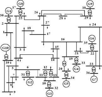
The implementation and execution of all four algorithms were carried out using MATLAB. Simulations were performed on five standard IEEE benchmark systems that have a different topology along with the ZI buses distributed differently. The utilization of ZI buses was in a manner that further relaxes the required number of PMUs. The topological characteristics of the simulated systems are shown in Table 2, while their single-line diagrams are indicated in Figures 11-15. All simulations were executed on a workstation equipped with an «CPU model» processor and «RAM» of RAM, running MATLAB «version» under «operating system». As O-SA and M-SA are stochastic, each algorithm was run «N» independent times on every test system; the execution times listed in Table 3 are the mean values over these runs, and the corresponding standard deviations of the SA-based methods are reported in Section 6. The bus, branch and zero-injection data of all benchmark systems were taken from the standard IEEE test-case data distributed with MATPOWER.
Figure 11. Single-line diagram of the IEEE 30-bus test system
Figure 12. Single-line diagram of the IEEE 14-bus test system
Figure 13. Single-line diagram of the IEEE 57-bus test system
Figure 14. Single-line diagram of the IEEE 118-bus test system
Figure 15. Single-line diagram of the New England 39-bus test system
Table 2. Test systems and zero-injection buses (ZIB)
|
System |
No. of Buses |
No. of Branches |
Zero-Injection Buses (ZIB) |
|
IEEE 14-bus |
14 |
20 |
7 |
|
IEEE 30-bus |
30 |
41 |
6, 9, 22, 25, 27, 28 |
|
IEEE 57-bus |
57 |
78 |
4, 7, 11, 21, 22, 24, 26, 34, 36, 37, 39, 40, 45, 46, 48 |
|
IEEE 118-bus |
118 |
179 |
5, 9, 30, 37, 38, 63, 64, 68, 71, 81 |
|
New England 39-bus |
39 |
46 |
1, 2, 5, 6, 9, 10, 11, 13, 14, 17, 19, 22 |
To account for best PMU counts and computation time of each method, an exhaustive study was made. Seeking observability of the network A · X ≥ I, i.e. all nodes are monitored, the placements of each algorithm in each system were validated prior to publishing the metrics; the table includes only those placements that comply with the rule. All case performance on each system is provided in Table 3 results, these identify the specific PMU buses selected in each case as observability evidence for the provided PMU counts. The DFS results in dense network coverage while the Recursive N-Security (RSN) algorithm picks a few nodes of high centrality.
Table 3. Simulation results of the Phasor Measurement Units (PMU) placement algorithms (selected buses and execution time)
|
System |
Algorithm |
PMUs |
Selected PMU Buses |
Exec. Time (s) |
|
14-bus |
DFS |
6 |
1, 4, 6, 8, 10, 14 |
0.009753 |
|
GTh |
6 |
1, 4, 6, 8, 10, 14 |
0.008370 |
|
|
O-SA |
4 |
2, 5, 6, 9 |
0.823044 |
|
|
M-SA |
5 |
1, 4, 6, 10, 14 |
0.104585 |
|
|
RSN |
3 |
2, 6, 9 |
0.240981 |
|
|
30-bus |
DFS |
10 |
1, 5, 6, 10, 11, 12, 18, 24, 26, 27 |
0.018140 |
|
GTh |
10 |
1, 5, 6, 10, 11, 12, 18, 24, 26, 27 |
0.024819 |
|
|
O-SA |
8 |
1, 5, 6, 10, 12, 18, 24, 27 |
0.277602 |
|
|
M-SA |
7 |
1, 5, 10, 12, 18, 24, 27 |
0.381523 |
|
|
RSN |
7 |
3, 7, 10, 12, 19, 24, 27 |
0.382163 |
|
|
57-bus |
DFS |
19 |
1, 4, 7, 9, 15, 19, 21, 24, 27, 30, 32, 36, 38, 39, 41, 46, 50, 52, 54 |
0.034562 |
|
GTh |
21 |
2, 4, 7, 9, 15, 16, 17, 19, 21, 24, 27, 30, 32, 36, 38, 39, 41, 46, 50, 52, 54 |
0.045720 |
|
|
O-SA |
19 |
1, 4, 7, 9, 15, 19, 21, 24, 27, 30, 32, 36, 38, 39, 41, 46, 50, 52, 54 |
0.615203 |
|
|
M-SA |
14 |
1, 6, 9, 15, 19, 21, 27, 29, 30, 32, 46, 50, 54, 56 |
2.458080 |
|
|
RSN |
12 |
1, 4, 13, 19, 27, 29, 30, 32, 38, 51, 54, 56 |
15.128233 |
|
|
118-bus |
DFS |
42 |
1, 5, 9, 12, 13, 17, 19, 21, 25, 28, 30, 32, 36, 37, 41, 43, 46, 49, 52, 57, 58, 59, 62, 65, 70, 72, 73, 77, 80, 83, 86, 89, 91, 93, 95, 100, 102, 105, 110, 115, 116, 118 |
0.137389 |
|
GTh |
42 |
1, 5, 9, 12, 13, 17, 19, 21, 25, 28, 30, 32, 36, 37, 41, 43, 46, 49, 52, 57, 58, 59, 62, 65, 70, 72, 73, 77, 80, 83, 86, 89, 91, 93, 95, 100, 102, 105, 110, 115, 116, 118 |
0.122252 |
|
|
O-SA |
40 |
1, 5, 9, 12, 13, 17, 19, 21, 25, 28, 30, 32, 36, 37, 41, 43, 46, 49, 52, 57, 58, 59, 62, 65, 70, 72, 77, 80, 83, 86, 89, 91, 93, 95, 100, 102, 105, 110, 115, 118 |
0.810999 |
|
|
M-SA |
37 |
1, 5, 9, 12, 13, 19, 21, 25, 28, 32, 36, 37, 41, 43, 46, 49, 52, 57, 58, 59, 62, 70, 72, 77, 80, 83, 86, 89, 91, 93, 95, 100, 102, 105, 110, 115, 118 |
6.245212 |
|
|
RSN |
36 |
1, 5, 9, 12, 13, 19, 21, 25, 29, 32, 36, 37, 41, 43, 46, 49, 53, 57, 58, 59, 62, 70, 72, 78, 80, 82, 84, 86, 89, 91, 94, 101, 105, 110, 115, 118 |
2.221426 |
|
|
New England 39-bus |
DFS |
16 |
2, 4, 6, 8, 10, 12, 16, 18, 20, 22, 26, 33, 36, 37, 38, 39 |
0.018402 |
|
GTh |
16 |
2, 4, 6, 8, 10, 12, 16, 18, 20, 22, 26, 33, 36, 37, 38, 39 |
0.024010 |
The absolute minimization tends to lower the capital cost, but it means a loss of topological observability redundancy. A generally acceptable monitoring system should have the relevant topological observability when any one of the relevant units is not in (or is failing in) proper operating order (N-1 contingencies). As a second check of compatibility of non-minimal topological redundancy, Table 4 reports topological redundancy metrics corresponding to the various assignments (subject to having no N-in extended ZI inference loops, for the given architecture). The indices are the Bus-based Observability Index average (BOI), the Sum of Redundancy Index (SORI), and the maximum fraction of the system which can be observed when the relevant single critical PMU is not available.
Table 4. Complementary structural redundancy metrics
|
System |
Algorithm |
Avg. BOI |
SORI |
Worst-Case Observed Ratio (1 PMU Lost) |
|
14-bus |
DFS |
1.571 |
22 |
0.857 |
|
14-bus |
RSN |
1.071 |
15 |
0.643 |
|
14-bus |
M-SA |
1.429 |
20 |
0.714 |
|
30-bus |
DFS |
1.433 |
43 |
0.867 |
|
30-bus |
RSN |
1.033 |
31 |
0.700 |
|
30-bus |
M-SA |
1.033 |
31 |
0.700 |
|
57-bus |
GTh |
1.421 |
81 |
0.930 |
|
57-bus |
RSN |
0.895 |
51 |
0.719 |
|
57-bus |
M-SA |
1.000 |
57 |
0.737 |
|
118-bus |
GTh |
1.610 |
190 |
0.966 |
|
118-bus |
RSN |
1.347 |
159 |
0.898 |
|
118-bus |
M-SA |
1.432 |
169 |
0.898 |
|
39-bus |
DFS |
1.462 |
57 |
0.923 |
|
39-bus |
RSN |
0.923 |
36 |
0.692 |
|
39-bus |
M-SA |
1.103 |
43 |
0.744 |
The highlighted advantage illustrates the trade-off between the solutions on operational parameters. Ranking the different algorithms by the number of PMU deployed, DFS and GTh regress to producing a high direct redundancy for the system (e.g. 96.6% for the case of the 118-bus one under the outage of a single PMU). The RSN algorithm scores the best short of coverage for specific locations at the expense of overexposing greater system area. The algorithms for deterministic grids with N-1 coverage security could add additional constraints to the M-SA and the RSN in the overlap of area coverage limits forcing further PMU under-coverage threshold. This could justify redundancy with explicit expectation of costs. To prove this full operational redundancy for the stochastic approaches (O-SA, M-SA) it still requires the assessment of the mean with standard deviation across runs. The mean and standard deviation for every case must therefore be reported before these outputs are relied upon in operational contexts, in order to confirm output stability.
The problem of OPP has been shown to be a complex one emphasizing the necessary tradeoff between minimum hardware and maximum observability of system structure. The immediate depth-first traversal approaches have not been found to yield a good solution, while the RSN is adept at discovering device minimums for complex networks. The M-SA is a robust stochastic method that yields nearly optimal counts while outperforming the RSN in less complex or sparser networks. As a result, grid managers must choose the appropriate algorithm for their placement policy: RSN for strict optimal financial deployment, or M-SA with additional N-1 securing topological constraints. Future research will endeavor to create hybrid algorithms combining the structural first tendencies of the RSN with stochastic type mutation methods to handle renewable-intermittency and more complex securing events.
[1] Mandal, A.K., De, S. (2023). Joint optimal PMU placement and data pruning for resource efficient smart grid monitoring. IEEE Transactions on Power Systems, 39(3): 5382-5392. https://doi.org/10.1109/TPWRS.2023.3320981
[2] Zhou, X., Wang, Y., Shi, Y., Jiang, Q., Zhou, C., Zheng, Z. (2024). Deep reinforcement learning-based optimal PMU placement considering the degree of power system observability. IEEE Transactions on Industrial Informatics, 20(6): 8949-8960. https://doi.org/10.1109/TII.2024.3378830
[3] Biswal, C., Sahu, B.K., Mishra, M., Rout, P.K. (2023). Real-time grid monitoring and protection: A comprehensive survey on the advantages of phasor measurement units. Energies, 16(10): 4054. https://doi.org/10.3390/en16104054
[4] Asadzadeh, B., Tousi, B., Galvani, S., Talavat, V. (2024). A robust state estimation by optimal placement of measurement units considering loads/renewable generations and measurements uncertainty. IET Renewable Power Generation, 18(6): 990-1006. https://doi.org/10.1049/rpg2.12983
[5] Islam, M.Z., Lin, Y., Vokkarane, V.M., Ogle, J. (2024). Observability-aware resilient PMU networking. IEEE Transactions on Power Systems, 40(1): 218-230. https://doi.org/10.1109/TPWRS.2024.3387338
[6] Perl, M., Sun, Z., Machlev, R., Belikov, J., Levy, K.Y., Levron, Y. (2024). PMU placement for fault line location using neural additive models—A global XAI technique. International Journal of Electrical Power & Energy Systems, 155: 109573. https://doi.org/10.1016/j.ijepes.2023.109573
[7] Wang, X., Xia, T., Li, Y., Mao, W. (2025). Two-stage optimal PMU placement for distribution systems. Measurement and Control, 58(6): 820-830. https://doi.org/10.1177/00202940241287641
[8] Ahmed, M.M., Amjad, M., Qureshi, M. A., Khan, M.O., Haider, Z.M. (2024). Optimal PMU placement to enhance observability in transmission networks using ILP and degree of centrality. Energies, 17(9): 2140. https://doi.org/10.3390/en17092140
[9] Almunif, A., Fan, L. (2020). Optimal PMU placement for modeling power grid observability with mathematical programming methods. International Transactions on Electrical Energy Systems, 30(2): e12182. https://doi.org/10.1002/2050-7038.12182
[10] Theodorakatos, N.P., Moschoudis, A.P., Lytras, M.D., Kantoutsis, K.T. (2023). Research on optimization procedure of PMU positioning problem achieving maximum observability based on heuristic algorithms. AIP Conference Proceedings, 2872(1): 120032. https://doi.org/10.1063/5.0162934
[11] Pal, A., Mishra, C., Vullikanti, A.K.S., Ravi, S.S. (2017). General optimal substation coverage algorithm for phasor measurement unit placement in practical systems. IET Generation, Transmission & Distribution, 11(2): 347-353. https://doi.org/10.1049/iet-gtd.2016.0553
[12] Okendo, E.O., Wekesa, C.W., Saulo, M.J. (2021). Optimal placement of phasor measurement unit considering system observability redundancy index: Case study of the Kenya power transmission network. Heliyon, 7(7): e07670. https://doi.org/10.1016/j.heliyon.2021.e07670
[13] Zhang, M., Wu, Z., Yan, J., Lu, R., Guan, X. (2022). Attack-resilient optimal PMU placement via reinforcement learning guided tree search in smart grids. IEEE Transactions on Information Forensics and Security, 17: 1919-1929. https://doi.org/10.1109/TIFS.2022.3173728
[14] Yuvaraju, V., Thangavel, S. (2022). Optimal phasor measurement unit placement for power system observability using teaching–learning based optimization. International Journal of Electrical Power & Energy Systems, 137: 107775. https://doi.org/10.1016/j.ijepes.2021.107775
[15] Vedik, B., Shiva, C.K. (2020). Multi-objective optimal placement of PMUS considering channel limitations and variable PMU costs using NSGA-II. Journal of Mechanics of Continua and Mathematical Sciences, 15(7): 148-167https://doi.org/10.26782/jmcms.2020.07.00012
[16] Nazari-Heris, M., Mohammadi-Ivatloo, B. (2015). Application of heuristic algorithms to optimal PMU placement in electric power systems: An updated review. Renewable and Sustainable Energy Reviews, 50: 214-228. https://doi.org/10.1016/j.rser.2015.04.152
[17] Pal, A., Sanchez-Ayala, G.A., Centeno, V.A., Thorp, J.S. (2013). A PMU placement scheme ensuring real-time monitoring of critical buses of the network. IEEE Transactions on Power Delivery, 29(2): 510-517. https://doi.org/10.1109/TPWRD.2013.2279172
[18] Manousakis, N.M., Korres, G.N., Georgilakis, P.S. (2012). Taxonomy of PMU placement methodologies. IEEE Transactions on Power Systems, 27(2): 1070-1077. https://doi.org/10.1109/TPWRS.2011.2179816
[19] Tangi, S., Gaonkar, D.N. (2021). Voltage estimation of active distribution network using PMU technology. IEEE Access, 9: 100436-100446. https://doi.org/10.1109/ACCESS.2021.3097001
[20] Abdolahi, A., Kalantari, N.T. (2022). State estimation of asymmetrical distribution networks by μ-PMU allocation: A novel stochastic two-stage programming. Electric Power Systems Research, 213: 108738. https://doi.org/10.1016/j.epsr.2022.108738
[21] Lei, X., Li, Z., Jiang, H., Yu, S.S., Chen, Y., Liu, B., Shi, P. (2025). Deep-learning based optimal PMU placement and fault classification for power system. Expert Systems with Applications, 292: 128586. https://doi.org/10.1016/j.eswa.2025.128586
[22] Korres, G.N., Manousakis, N.M. (2012). Observability analysis and restoration for state estimation using SCADA and PMU data. In 2012 IEEE Power and Energy Society General Meeting, San Diego, CA, USA, pp. 1-8. https://doi.org/10.1109/PESGM.2012.6345096
[23] Peng, Y., Wu, Z., Gu, W., Zhou, S., Liu, P. (2023). Optimal Micro-PMU placement for improving state estimation accuracy via mixed-integer semidefinite programming. Journal of Modern Power Systems and Clean Energy, 11(2): 468-478. https://doi.org/10.35833/mpce.2021.000615
[24] Blair, S.M., Syed, M.H., Roscoe, A.J., Burt, G.M., Braun, J.P. (2019). Measurement and analysis of PMU reporting latency for smart grid protection and control applications. IEEE Access, 7: 48689-48698. https://doi.org/10.1109/ACCESS.2019.2903929
[25] Tangi, S., Gaonkar, D.N., Nuvvula, R.S., Kumar, P.P., Colak, I., Tazay, A.F., Mosaad, M.I. (2024). Smart distribution network voltage estimation using PMU technology considering zero injection constraints. Plos One, 19(3): e0293616. https://doi.org/10.1371/journal.pone.0293616
[26] Ghamsari-Yazdel, M., reza Najafi, H., Amjady, N. (2019). Novel notions of zero injection property of buses in optimal PMU location with efficient observability enhancement focusing on security concepts. Electric Power Systems Research, 169: 24-34. https://doi.org/10.1016/j.epsr.2018.12.009
[27] Ali, A., Abdul Wahab, N.I., Othman, M.L., Farade, R.A., Samkari, H.S., Allehyani, M.F. (2025). Optimal µ-PMU placement and voltage estimation in distribution networks: Evaluation through multiple case studies. Sustainability, 17(24): 11036. https://doi.org/10.3390/su172411036