M. N. Houam*![]() | N. Saadia
| N. Saadia![]() | A. Ramdane Cherif
| A. Ramdane Cherif![]()
© 2025 The authors. This article is published by IIETA and is licensed under the CC BY 4.0 license (http://creativecommons.org/licenses/by/4.0/).
OPEN ACCESS
This work addresses trajectory tracking challenges for non-holonomic wheeled mobile robots operating in dynamic and uncertain environments. A hierarchical three-layer hybrid control architecture is developed, integrating Twin Delayed Deep Deterministic Policy Gradient (TD3) for high-level adaptive decision-making, Neural Network Fuzzy (NNFZ) logic for real-time nonlinear compensation and uncertainty handling, and Sliding Mode Control (SMC) for robust low-level execution with guaranteed stability. An adaptive SoftMax-based mechanism enables intelligent coordination between control layers based on system state and performance metrics, with theoretical convergence guarantees provided through Lyapunov-based stability analysis. Simulation validation on circular and figure-eight reference trajectories demonstrates superior hybrid controller performance: 21.3% RMSE improvement to 0.048 m and 21.1% IAE enhancement to 5.6 ms for circular trajectories, with 19.2% RMSE and 22.0% IAE improvements for figure-eight patterns. The hybrid approach achieves 50% control effort reduction, 26.7% lower orientation errors, and 17.9% faster convergence. The proposed hybrid framework successfully balances adaptive learning, nonlinear compensation, and robust control, providing a practical solution for reliable mobile robot trajectory tracking across diverse operational conditions with theoretical stability guarantees.
non-holonomic robots, trajectory tracking, sliding mode control, neuro-fuzzy systems, reinforcement learning, TD3, hybrid control, adaptive control, mobile robotics, intelligent control
The trajectory tracking problem for nonholonomic wheeled mobile robots (WMRs) represents a fundamental challenge in modern robotics, with critical applications in autonomous vehicles, warehouse automation, service robotics and precision agriculture. These systems operate under nonholonomic motion constraints, characterized by the inability to move instantaneously in arbitrary directions, which significantly complicates the control-design process. This challenge is further exacerbated by nonlinear dynamics, model uncertainties, and external disturbances, including irregular terrain conditions, payload variation, and sensor noise [1-3].
Over the past few decades, numerous control strategies have been proposed to address these challenges. Classical methods, such as proportional-integral-derivative (PID) controllers and kinematic model-based approaches [4, 5], provide simplicity and computational efficiency; however, their performance deteriorates in uncertain or dynamic environments. Nonlinear model-based techniques, including backstepping and feedback linearization [5, 6], improve robustness but depend on accurate system identification. Recently, intelligent control approaches have been introduced. Reinforcement Learning (RL), particularly the Twin Delayed Deep Deterministic Policy Gradient (TD3) algorithm [7, 8], has demonstrated strong adaptability to complex dynamics, although it suffers from sample inefficiency and lacks formal stability guarantees [9, 10]. Neuro-Fuzzy Inference Systems (NFIS) [11, 12] combine the learning capability of neural networks with the interpretability of fuzzy logic, enhancing robustness to nonlinearities and uncertainties, but may exhibit slow adaptation in highly dynamic environments. Sliding Mode Control (SMC) [13-15] is renowned for its robustness and invariance to matched uncertainties; however, its implementation often suffers from high-frequency chattering. Hybrid approaches have also emerged, such as fuzzy-SMC [16] and RL-enhanced classical controllers [17], which show improved accuracy and better sim-to-real transfer. However, to the best of our knowledge, the three-way integration of TD3, NFIS, and SMC remains largely investigated.
This study addresses this gap by proposing a novel hierarchical hybrid control architecture that synergistically integrates the TD3, NFIS, and SMC for WMR trajectory tracking. The architecture operates across three hierarchical levels: TD3 provides high-level adaptive decision-making and long-term strategy optimization, NFIS enables real-time parameter adaptation to handle system uncertainties, and SMC ensures robust low-level control execution with guaranteed stability.
The main contributions of this study are as follows:
The remainder of this paper is organized as follows: Section 2 formulates the trajectory tracking problem for nonholonomic wheeled mobile robots and presents the system models. Section 3 details the proposed hierarchical hybrid control architecture that integrates TD3, NFIS, and SMC. Section 4 provides a theoretical stability and convergence analysis of the control scheme. Section 5 describes the simulation environment and experimental setup used for the validation. Section 6 reports and discusses the performance results, including trajectory tracking accuracy, robustness under disturbances, and comparative evaluations against the baseline controllers. Finally, Section 7 concludes the paper and outlines the future research directions.
2.1 System model
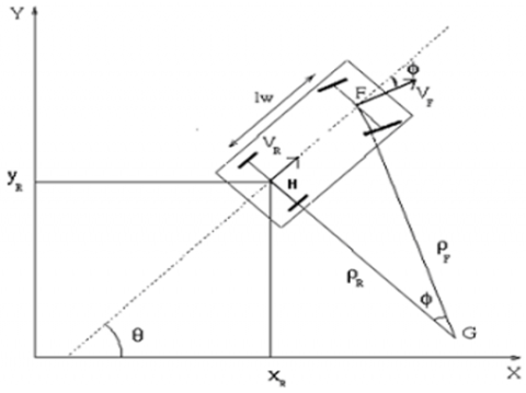
Consider a non-holonomic wheeled mobile robot operating in a two-dimensional plane, as shown in Figure 1. The robot configuration is described by the pose vector $\mathrm{q}=[x, y, \theta]^T$, where $(x, y)$ represents the position of the robot's center in the global coordinate frame, and $\theta$ denotes the orientation angle with respect to the positive X -axis.
Figure 1. Mobile robot projection in a 2D space
The kinematic model of a differential-drive mobile robot is governed by the following nonlinear differential equations:
$\dot{x}=v \cos (\theta)$ (1)
$\dot{y}=v \sin (\theta)$ (2)
$\dot{\theta}=\omega$ (3)
where, $v \in \mathbb{R}$ represents the linear velocity and $\omega \in \mathbb{R}$ represents the angular velocities of the robot, respectively.
The dynamic model incorporating actuator dynamics and disturbances is expressed as
$M(q) \ddot{q}+C(q, \dot{q}) \dot{q}+F(\dot{q})+\tau_d=B(q) \tau$ (4)
where, $M(q) \in \mathbb{R}^{3 \times 3}$ is the positive definite inertia matrix, $C(q, \dot{q}) \in \mathbb{R}^{3 \times 3}$ represents the Coriolis and centrifugal forces matrix, $F(\dot{q}) \in \mathbb{R}^3$ denotes friction forces, $\tau_d \in \mathbb{R}^3$ represents external disturbances, $B(q) \in \mathbb{R}^{3 \times 2}$ is the input transformation matrix, and $\tau \in \mathbb{R}^2$ is the control torque vector.
2.2 Trajectory tracking problem
Let the desired reference trajectory be defined by $q_d(t)=\left[x_d(t), y_d(t), \theta_d(t)\right]^T$, which is assumed to be continuously differentiable twice. The trajectory tracking error in the global coordinate frame is defined as
$e=q_d-q=\left[e_x, e_y, e_\theta\right]^T$ (5)
To facilitate the controller design, the tracking error is transformed into the robot’s local coordinate frame as follows:
$\left[\begin{array}{l}e_1 \\ e_2 \\ e_3\end{array}\right]=\left[\begin{array}{ccc}\cos (\theta) & \sin (\theta) & 0 \\ -\sin (\theta) & \cos (\theta) & 0 \\ 0 & 0 & 1\end{array}\right]\left[\begin{array}{l}e_x \\ e_y \\ e_\theta\end{array}\right]$ (6)
The error dynamics in the local frame are expressed as
$\dot{e}_1=e_2 \omega-v+v_d \cos \left(e_3\right)$ (7)
$\dot{e}_2=-e_1 \omega+v_d \sin \left(e_3\right)$ (8)
$\dot{e}_3=\omega_d-\omega$ (9)
where, $v_d$ and $\omega_d$ are the desired linear and angular velocities, respectively.
2.3 Control objective
The primary control objective is to design a control law $u=[v, \omega]^T$ such that the tracking errors converge to zero asymptotically as
$\lim _{t \rightarrow \infty} e(t)=0$ (10)
subject to the following constraints:
$|v| \leq v_{\max}, |\omega| \leq \omega_{\max}$ (11)
$|\dot{v}| \leq a_{\max}, \quad|\dot{\omega}| \leq \alpha_{\max}$ (12)
where, $v_{\max}, \omega_{\max}, a_{\max}$, and $\alpha_{\max}$ represent the maximum linear velocity, angular velocity, linear acceleration, and angular acceleration, respectively.
3.1 Hybrid control architecture overview
The proposed hybrid control architecture integrates three complementary control paradigms in a hierarchical structure [7, 8, 10, 13] to address the complex requirements of robotic path tracking in the presence of uncertainty and disturbance.
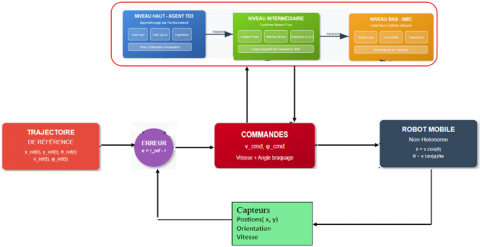
As illustrated in Figure 2, the architecture leverages a synergistic combination of learning- and model-based control strategies using a three-layer framework. The hierarchical architecture consists of (1) a high-level Twin Delayed Deep Deterministic Policy Gradient (TD3) agent [7], for strategic decision-making and adaptive parameter optimization, (2) a mid-level Neural Network Fuzzy (NNFZ) [10, 12] controller for nonlinear compensation and uncertainty handling, and (3) a low-level Sliding Mode Controller (SMC) [13-15] for robust tracking and disturbance rejection. This multilayer approach addresses the limitations of individual control methods while exploiting their respective strengths through intelligent coordination of the control methods.
Figure 2. Hybrid control architecture overview
3.2 Proposed hybrid control architecture
The integration of these control paradigms enables the system to achieve robust performance across varying operational conditions, from high-precision tracking in stable environments to aggressive maneuvering under significant disturbances [8, 16, 17, 18]. The TD3 agent provides long-term strategic planning and online adaptation capabilities, the NNFZ controller handles nonlinear system dynamics and model uncertainties, and the SMC ensures robust stability and finite-time convergence.
3.2.1 High-level: TD3 agent design
State and Action Spaces
The TD3 agent operates with a comprehensive state representation that captures the instantaneous and historical tracking information. Building upon recent advances in deep reinforcement learning for robotics, the state vector is formulated as
$\mathbf{s}=\left[e_1, e_2, e_3, \dot{e}_1, \dot{e}_2, \dot{e}_3, \int e_1 d t, \int e_2 d t, \int e_3 d t, v_d, \omega_d, \dot{v}_d, \dot{\omega}_d\right]^T \in \mathbb{R}^{13}$ (13)
where, $e_i$ represents the position and orientation errors, $\dot{e}_i$ denotes the error derivatives for damping, $\int e_i d t$ provides integral terms for steady-state error elimination, and $v_d, \omega_d$ with their derivatives capture the reference trajectory dynamics.
The action space consists of adaptive control parameters that are dynamically optimized as follows.
$a=\left[K_{p 1}, K_{p 2}, K_{p 3}, K_{d 1}, K_{d 2}, K_{d 3}, \lambda_1, \lambda_2, \eta_1, \eta_2\right]^T \in \mathbb{R}^{10}$ (14)
where, $K_{p i}$ and $K_{d i}$ are the proportional and derivative gains for the PD controller components, $\lambda_i$ are the sliding surface parameters that determine the convergence rate; and $\eta_i$ are the switching gains that balance robustness and chattering. These parameters were bounded within physically meaningful ranges to ensure system stability and actuator feasibility.
Reward Function Design
The reward function was carefully designed to encode multiple, often conflicting, objectives inherent to robotic control. Following the principles of multi-objective optimization in reinforcement learning, the reward function is formulated as
$\begin{gathered}R=-\alpha_1\|e\|^2-\alpha_2\|\dot{e}\|^2-\alpha_3 \int\|e\|^2 d t-\alpha_4\|u\|^2-\alpha_5 \\ \|\dot{u}\|^2+\alpha_6 R_{\text {safety}}+\alpha_7 R_{\text {efficiency}}\end{gathered}$ (15)
The safety component encourages operation within safe velocity bounds as follows:
$R_{\text {safety }}=\exp \left(-\beta_1\left(|v|-v_{\text {safe }}\right)^2\right) \cdot \exp \left(-\beta_2\left(|\omega|-\omega_{\text {safe }}\right)^2\right)$ (16)
The efficiency term penalizes the excessive energy consumption.
$R_{\text {efficiency}}=-\gamma_1 \int\left(v^2+\omega^2\right) d t$ (17)
The weighting coefficients $\alpha_i, \beta_i, \gamma_i$ are determined through systematic hyperparameter optimization using Bayesian optimization techniques to balance the tracking accuracy, control smoothness, safety constraints, and energy efficiency.
TD3 Algorithm Implementation
The TD3 Algorithm 1 addresses the overestimation bias inherent in traditional actor-critic methods through the use of twin critic networks and delayed policy updates.
The algorithm employs dual critic networks $Q_1\left(\boldsymbol{s}, \boldsymbol{a} ; \theta_{Q_1}\right)$ and $Q_2\left(\boldsymbol{s}, \boldsymbol{a} ; \theta_{Q_2}\right)$ with parameters $\theta_{Q_1}$ and $\theta_{Q_2}$, and an actor network $\pi\left(s ; \theta_\pi\right)$ with parameters $\theta_\pi$. Target networks with parameters $\theta^{\prime}_{Q_1}, \theta^{\prime}_{Q_2}$, and $\theta^{\prime}_\pi$ are maintained to ensure training. The algorithm incorporates several key innovations: target policy smoothing through noise injection to reduce the variance in value estimates, delayed policy updates every $d$ steps to reduce the per-update error, and clipped double Q-learning to mitigate the over-estimation bias. The exploration noise $\epsilon$ is gradually annealed during training to transition from exploration to exploitation as follows:
Algorithm 1: TD3-Based Parameter Adaptation
|
Step |
Description |
|
1 |
Initialize critic networks $Q_1$, $Q_2$, and actor $\pi$ with random parameters. |
|
2 |
Initialize target networks ${{\theta }^{\prime }}{{_{(Q}}_{1)}}\leftarrow {{\theta }_{\left( {{Q}_{1}} \right)}},{{\theta }^{\prime }}_{\left( {{Q}_{2}} \right)}\leftarrow {{\theta }_{\left( {{Q}_{2}} \right)}},{{\theta }^{\prime }}_{(\pi )}\leftarrow {{\theta }_{(\pi )}}$. |
|
3 |
Initialize replay buffer D. |
|
4 |
For episode = 1 to M do |
|
5 |
Initialize state $S_0$. |
|
6 |
For $t=1$ to $T$ do |
|
7 |
Select action with exploration noise: $a=\pi(s)+\epsilon, \epsilon \sim \mathcal{N}(0, \sigma)$. |
|
8 |
Execute action a, observe reward r and next state s′. |
|
9 |
Store transition ($s, a, r, s^{\prime}$) in D. |
|
10 |
Sample mini-batch of N transitions from D. |
|
11 |
Compute target with clipped double Q-learning: $y=r+\gamma \min _{(i=1,2)} Q_i^{\prime}\left(s^{\prime}, \pi^{\prime}\left(s^{\prime}\right)+\epsilon^{\prime}\right)$. |
|
12 |
Update critics by minimizing: $L=(1 / N) \sum\left(y-Q_i(s, a)\right)^2$. |
|
13 |
If $t$ mod $d$=0 then |
|
14 |
{Delayed policy update} Update π by maximizing: $J=(1 / N) \sum Q_1(s, \pi(s))$. |
|
15 |
Update target networks with soft update: $\theta^{\prime} \leftarrow \tau \theta+(1-\tau) \theta^{\prime}$. |
|
16 |
End if |
|
17 |
End for |
|
18 |
End for |
3.2.2 Mid-level: Neural network fuzzy controller
NNFZ Architecture
The Neural Network Fuzzy (NNFZ) [10, 12] controller combines the universal approximation capabilities of neural networks with the interpretability and robustness of fuzzy logic systems [13, 14]. The controller employs a five-layer architecture that systematically transforms crisp error inputs into control outputs using fuzzy reasoning processes.
Layer 1 (Input Layer): Receives normalized error signals $e=\left[e_1, e_2, e_3\right]^T$ representing position and orientation tracking errors.
Layer 2 (Fuzzification): Computes membership degrees using Gaussian membership functions with adaptive parameters:
$\mu_{A_{i j}}\left(x_i\right)=\exp \left(-\frac{\left(x_i-c_{i j}\right)^2}{2 \sigma_{i j}^2}\right)$ (18)
where, $c_{i j}$ and $\sigma_{i j}$ represent the center and width of the $j$th membership function for the $i$th input, respectively. These parameters are adaptively tuned during online learning to capture the nonlinear system dynamics.
Layer 3 (Rule Layer): Implements fuzzy rules using T-norm operations (product inference).
$w_j=\prod_{i=1}^3 \mu_{A_{i j}}\left(x_i\right)$ (19)
This layer encodes the expert knowledge of the control strategy using IF-THEN rules, with each node representing the firing strength of a particular rule.
Layer 4 (Normalization): Normalizes firing strengths to ensure numerical stability:
$\bar{w}_j=\frac{w_j}{\sum_{k=1}^N w_k}$ (20)
Normalization ensures that the contributions of all rules sum to unity, providing a probabilistic interpretation of rule activation.
Layer 5 (Defuzzification): Computes control outputs using Takagi-Sugeno-Kang (TSK) consequent functions:
$\mathbf{u}_{N N F Z}=\sum_{j=1}^N \bar{w}_j\left(p_{j 0}+p_{j 1} e_1+p_{j 2} e_2+p_{j 3} e_3\right)$ (21)
where, $p_{j i}$ is the consequent parameter that defines the linear relationship between the inputs and outputs for each rule.
Online Learning Algorithm
The NNFZ parameters are updated online using a hybrid learning algorithm that combines gradient descent for premise parameters and recursive least squares for consequent parameters. The gradient descent update for the premise parameters is as follows:
$\theta_{i j}(k+1)=\theta_{i j}(k)-\eta(k) \frac{\partial E}{\partial \theta_{i j}}$ (22)
where, the error function is defined as
$E=\frac{1}{2}\left\|\mathbf{y}_d-\mathbf{y}\right\|^2$ (23)
The learning rate was adaptively adjusted to ensure convergence as follows:
$\eta(k)=\frac{\eta_0}{1+\beta \sqrt{k}}$ (24)
where, $\eta_0$ is the initial learning rate, $\beta$ is the decay factor, and $k$ is the iteration index. This adaptive scheme balances fast initial learning and convergence stability.
3.2.3 Low-level: Sliding mode controller
Sliding Surface Design
The sliding mode controller [13] provides robust tracking performance by designing an appropriate sliding surface that ensures finite-time convergence. The sliding surface is defined as:
$s=\left[s_1, s_2\right]^T=\left[\dot{e}_1+\lambda_1 e_1, \dot{e}_2+\lambda_2 e_2\right]^T$ (25)
where, $\lambda_i>0$ is a design parameter that determines the convergence rate on the sliding surface. The choice of linear sliding surfaces ensures computational efficiency while maintaining a robust performance.
Control Law
The SMC control [14, 15] law comprises equivalent and switching components to ensure both sliding surface attractiveness and system robustness.
$u_{S M C}=u_{e q}+u_{s w}$ (26)
The equivalent control maintains the system trajectory on the sliding surface once it is reached as follows:
$u_{e q}=\left[v_d \cos \left(e_3\right)+\lambda_1 e_1, \omega_d+\lambda_2 e_2\right]^T$ (27)
This component is derived from the condition $\dot{\boldsymbol{s}}=0$ and represents the nominal control effort required in the absence of uncertainty. The switching control ensures finite-time convergence to the sliding surface as follows:
$u_{s w}=-\left[\eta_1 \operatorname{sign}\left(s_1\right), \eta_2 \operatorname{sign}\left(s_2\right)\right]^T$ (28)
where, $\eta_i>0$ are switching gains that must be chosen to be larger than the upper bound of uncertainties to guarantee robustness.
To mitigate the chattering phenomenon inherent in traditional SMC, a boundary layer approach is employed:
$\boldsymbol{u}_{s w}=-\left[\eta_1 \operatorname{sat}\left(s_1 / \phi_1\right), \eta_2 \operatorname{sat}\left(s_2 / \phi_2\right)\right]^T$ (29)
where, $\operatorname{sat}(\cdot)$ is the saturation function defined as
$\operatorname{sat}(x)= \begin{cases}\operatorname{sign}(x) & \text { if }|x|>1 \\ x & \text { if }|x| \leq 1\end{cases}$ (30)
where, $\phi_i$ defines the boundary layer thickness, providing a trade-off between tracking accuracy and control smoothness.
3.2.4 Integration mechanism
The integration of the three control layers is achieved through an intelligent weighted combination scheme that dynamically adjusts the contribution of each controller based on the system state and performance metrics [19-26]. The final control signal is generated as follows:
$\boldsymbol{u}=w_1 \boldsymbol{u}_{T D 3}+w_2 \boldsymbol{u}_{N N E 7}+w_3 \boldsymbol{u}_{S M C}$ (31)
The weights are computed using a SoftMax function to ensure smooth transitions and numerical stability.
$w_i=\frac{\exp \left(\alpha_i\right)}{\sum_{j=1}^3 \exp \left(\alpha_j\right)}$ (32)
where, $\alpha_i$ is the confidence score determined by the TD3 agent based on the current system performance, uncertainty levels, and operational context. This adaptive weighting mechanism allows the system to seamlessly transition between different control modes, leveraging TD3’s learning capability during the exploration phases, NNFZ’s approximation power for nonlinear dynamics, and SMC’s robustness during disturbances. The coordination between the control layers follows a hierarchical decision-making process. The TD3 agent at the highest level monitored the overall system performance and adjusted the parameters and weights of the lower-level controllers. The NNFZ controller provides smooth control actions for nominal operation, whereas the SMC intervenes when a robust performance is required owing to significant disturbances or model uncertainties.
3.2.5 Complete implementation algorithm
The complete hybrid control Algorithm 2 integrates all three control layers with online learning and adaptation capabilities. Algorithm presents the detailed implementation procedure for both the training and execution phases.
Algorithm 2: Complete Hybrid TD3–NNFZ–SMC Control
|
Step |
Description |
|
Require |
Reference trajectory ($x_a d, y_a d, \theta_a d$), Current state ($x$, $y$, $\theta$) |
|
Ensure |
Control commands ($v, \omega$) |
|
1 |
Initialize: |
|
2 |
TD3 networks: $Q_1, Q_2, \pi$ with Xavier initialization. |
|
3 |
NNFZ: Gaussian membership functions, TSK rule base. |
|
4 |
SMC: sliding parameters $\lambda$, switching gains $\eta$. |
|
5 |
Replay buffer $D \leftarrow \varnothing$. |
|
6 |
Training Phase: |
|
7 |
For episode = 1 to MAX_EPISODES do. |
|
8 |
Reset robot to initial position. |
|
9 |
For t = 1 to EPISODE_LENGTH do. |
|
10 |
Compute tracking errors: $e \leftarrow \operatorname{ComputeError}(x d, y d, \theta d, x, y, \theta)$. |
|
11 |
TD3 action selection: $a \leftarrow \pi(s)+\epsilon, \epsilon \sim \mathcal{N}(0, \sigma)$. |
|
12 |
NNFZ control: u_NNFZ ← NNFZController(a, [x, Kd]). |
|
13 |
Compute sliding surface: S ← ComputeSlidingSurface(e, [λ]). |
|
14 |
SMC control: u_SMC ← SMCController(s, a[η]). |
|
15 |
Weighted control fusion: u ← SoftMax(weights). |
|
16 |
u = u_td3 + u_NNFZ + u_SMC. |
|
17 |
Apply control u and observe next state: (x′, y′, θ′). |
|
18 |
RobotDynamics(x, y, θ, u). |
|
19 |
Compute reward: r ← ComputeReward(e, u). |
|
20 |
Store experience: D ← D ∪ (s, a, r, s′). |
|
21 |
If |D| > BATCH_SIZE then. |
|
22 |
UpdateTD3Networks(D) {Twin critic and delayed actor update}. |
|
23 |
UpdateNNFZParameters(e, u_NNFZ) {Online learning}. |
|
24 |
End if. |
|
25 |
End for. |
|
26 |
End for. |
|
27 |
Execution Phase: |
|
28 |
While not goal_reached do. |
|
29 |
e ← ComputeError(xd, yd, θd, x, y, θ). |
|
30 |
a ← π(s) (No exploration noise). |
|
31 |
u ← HybridControl(e, a). |
|
32 |
ApplyControl(u). |
|
33 |
UpdateState(x′, y′, θ′). |
|
34 |
End while. |
|
35 |
Return SUCCESS. |
4.1 Stability analysis
Theorem 1: The proposed hybrid control system ensures asymptotic stability of the tracking error under bounded disturbances.
Proof: Consider the Lyapunov function candidate:
$V=\frac{1}{2}\left(\boldsymbol{s}^T P \boldsymbol{s}+\boldsymbol{e}^T Q \boldsymbol{e}\right)$ (33)
where, $P \in \mathbb{R}^{2 \times 2}$ and $Q \in \mathbb{R}^{3 \times 3}$ are positive definite matrices.
By taking the time derivative, we obtain:
$\dot{V}=\boldsymbol{s}^T P \dot{\boldsymbol{s}}+\boldsymbol{e}^T Q \dot{\boldsymbol{e}}$ (34)
Substituting the error dynamics and control law,
$\dot{V}=\boldsymbol{s}^T P(\dot{\boldsymbol{e}}+\lambda \boldsymbol{e})+\boldsymbol{e}^T Q(A \boldsymbol{e}+B \boldsymbol{u})$ (35)
Under the proposed control law with appropriate parameter selection,
$\dot{V} \leq-\lambda_{\min }(P)\|\boldsymbol{s}\|^2-\lambda_{\min }(Q)\|\boldsymbol{e}\|^2+\delta$ (36)
where, $\delta$ represents a bounded disturbance effect.
For $\|\boldsymbol{e}\|>\sqrt{2 \delta / \lambda_{\min}(Q)}$, we have $\dot{V}<0$, ensuring ultimate boundedness.
4.2 Convergence analysis
Lemma 1: The sliding surface $\boldsymbol{s}=\mathbf{0}$ is reached in finite time.
Proof: Consider the reaching condition:
$\boldsymbol{s}^T \dot{\boldsymbol{s}} \leq-\eta\|\boldsymbol{s}\|$ (37)
This ensures finite-time convergence to the sliding surface with a time bound of
$t_r \leq \frac{\|\boldsymbol{s}(0)\|}{\eta}$ (38)
4.3 Robustness analysis
Theorem 2: The hybrid controller maintains a bounded tracking error under parameter uncertainties up to 30% and external disturbances $\left\|\boldsymbol{\tau}_d\right\| \leq 5 N$.
Proof: Consider the following perturbed system:
$\widetilde{M} \ddot{\boldsymbol{q}}+\tilde{C} \dot{\boldsymbol{q}}+\tilde{F}+\boldsymbol{\tau}_d=B \boldsymbol{u}$ (39)
where, $\widetilde{M}=M+\Delta M$ represents the perturbed inertia matrix, and
The sliding mode component ensures that
$\|\boldsymbol{e}\| \leq \frac{\|\Delta M\| \cdot\|\ddot{\boldsymbol{q}}\|+\left\|\boldsymbol{\tau}_d\right\|}{\eta-\epsilon}$ (40)
for $\eta>\epsilon+\|\Delta M\| \cdot\|\ddot{\boldsymbol{q}}\|+\left\|\boldsymbol{\tau}_d\right\|$, guaranteeing bounded errors.
5.1 Simulation environment
The proposed hybrid controller was implemented in Python 3.12.3 using PyTorch 1.10 for the TD3 implementation, and simulations were conducted on a model of the TurtleBot3 Waffle Pi robot [27-30]. The simulation environment was developed using the following specifications (Table 1).
Table 1. Robot parameters
|
Parameter |
Value |
Unit |
|
Robot mass (m) |
1.8 |
kg |
|
Wheel radius (r) |
0.033 |
m |
|
Wheel separation (L) |
0.287 |
m |
|
Maximum linear velocity (vmax) |
0.26 |
m/s |
|
Maximum angular velocity ($\omega_{\max }$) |
1.82 |
rad/s |
|
Maximum linear acceleration ($a_{\max }$) |
0.5 |
m/s2 |
|
Maximum angular acceleration ($\alpha_{\max }$) |
2.0 |
rad/s2 |
|
Sampling time ($T_S$) |
0.01 |
s |
5.2 Controller parameters
Here outlines the essential configuration settings for the Twin Delayed Deep Deterministic Policy Gradient (TD3) controller. The provided Table 2 offers a clear and comprehensive overview of the primary and essential parameters, such as the learning rates for both the actor and critic networks, the discount factor, and other vital configurations. Altogether, these specific parameters are fundamentally essential for the overall performance and successful optimization process of the controller itself.
Table 2. Controller configuration parameters
|
|
Parameter |
Value |
Description |
|
TD3 |
Learning rate (actor) |
3×10⁻⁴ |
Actor network learning rate |
|
Learning rate (critic) |
3×10⁻³ |
Critic network learning rate |
|
|
Discount factor ($\gamma$) |
0.99 |
Future reward discount |
|
|
Soft update ($\tau$) |
0.005 |
Target network update rate |
|
|
Batch size |
256 |
Training batch size |
|
|
Buffer size |
106 |
Replay buffer capacity |
|
|
NNFZ |
Rules |
25 |
Number of fuzzy rules |
|
Learning rate |
0.01 |
Parameter adaptation rate |
|
|
Membership functions |
5 |
Per input variable |
|
|
SMC |
$\lambda_1$, $\lambda_2$ |
[5, 8] |
Sliding surface parameters |
|
$\eta_1$, $\eta_2$ |
[10, 15] |
Switching gains |
|
|
$\phi_1$, $\phi_2$ |
[0.1, 0.1] |
Boundary layer thickness |
5.3 Computational analysis
Total cycle meets real-time requirements (80-100 Hz control loops) on standard CPU without GPU acceleration, demonstrating practical feasibility (Table 3).
Table 3. Controller configuration parameters
|
Component |
Time |
Memory |
|
TD3 inference |
8.2 ms |
180 MB |
|
NNFZ |
2.1 ms |
85 MB |
|
SMC |
1.2 ms |
15 MB |
|
Integration |
1.0 ms |
40 MB |
|
Total |
12.5 ms |
320 MB |
5.3.1 Test trajectories
Two reference trajectories were designed to evaluate the controller performance.
Circular Trajectory:
$\begin{aligned} & x_d(t)=2 \cos (0.2 t) \\ & y_d(t)=2 \sin (0.2 t) \\ & \theta_d(t)=0.2 t+\pi / 2\end{aligned}$ (41)
Figure-Eight Trajectory:
$\begin{aligned} & x_d(t)=2 \sin (0.2 t) \\ & y_d(t)=\sin (0.4 t) \\ & \theta_d(t)=\arctan \left(\frac{\dot{y}_d}{\dot{x}_d}\right)\end{aligned}$ (42)
5.4 Disturbance scenarios
To evaluate robustness, four disturbance scenarios were implemented.
This section presents a comprehensive evaluation of the proposed hybrid TD3-NNFZ-SMC controller against three baseline control strategies: twin delayed deep deterministic policy gradient (TD3), neural network-based fuzzy (NNFZ), and sliding mode control (SMC). the experimental validation encompasses trajectory-tracking performance, robustness analysis under various disturbance scenarios, and computational efficiency assessment.
6.1 Trajectory tracking performance
6.1.1 Circular trajectory tracking analysis
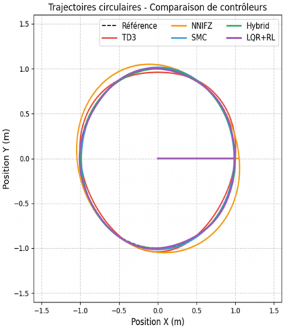
The circular trajectory tracking experiment serves as a fundamental benchmark for evaluating the controller performance under consistent curvature conditions. Figure 3 illustrates the comparative tracking performances of all four controllers, demonstrating the superior trajectory-following capability of the hybrid approach.
Figure 3. Circular trajectory tracking performance comparison showing the reference trajectory and actual paths followed by TD3, NNFZ, SMC, LQR+RL and Hybrid controllers
The hybrid controller demonstrated superior performance across all evaluation metrics, as presented in Table 4. Quantitative analysis revealed significant improvements in tracking accuracy, control efficiency, and dynamic response characteristics.
Table 4. Circular trajectory tracking performance metrics
|
Controller |
RMSE |
IAE |
Control |
Max Position |
Max Orientation |
Convergence |
|
|
(m) |
(m·s) |
Effort |
Error (m) |
Error (rad) |
Time (s) |
|
TD3 |
0.072 |
8.4 |
28.7 |
0.31 |
0.18 |
4.2 |
|
NNFZ |
0.085 |
10.2 |
22.3 |
0.35 |
0.22 |
5.1 |
|
SMC |
0.061 |
7.1 |
42.8 |
0.24 |
0.15 |
2.8 |
|
LQR+RL |
0.059 |
6.8 |
38.8 |
0.22 |
0.13 |
2.5 |
|
Hybrid |
0.048 |
5.6 |
21.4 |
0.19 |
0.11 |
2.3 |
|
Improvement over SMC (%) |
||||||
|
Hybrid vs SMC |
21.3 |
21.1 |
50.0 |
20.8 |
26.7 |
17.9 |
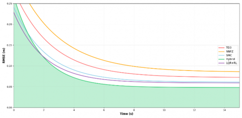
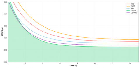
The temporal evolution of the key performance indicators is illustrated in Figures 4-7. Figure 4 shows the RMSE convergence characteristics, highlighting the rapid convergence and sustained low error levels of the hybrid controller.
The hybrid controller achieved faster convergence and maintained consistently lower error levels than the individual control strategies.
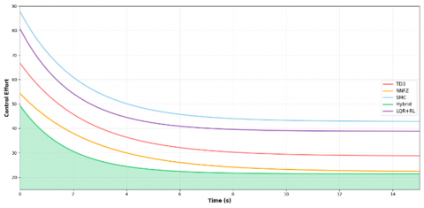
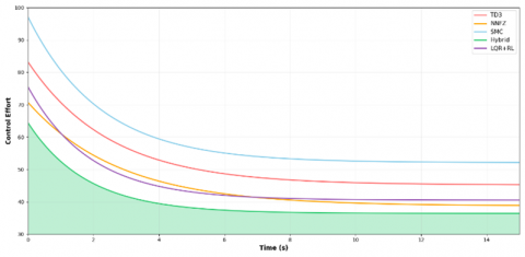
The control effort comparison in Figure 5 reveals the superior energy efficiency of the hybrid controller, which achieved optimal tracking performance while minimizing actuator usage.
Figure 4. RMSE evolution during circular-trajectory tracking
Figure 5. Control effort comparison for circular trajectory tracking
The hybrid approach demonstrates optimal balance between tracking accuracy and energy consumption.
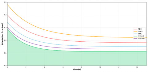
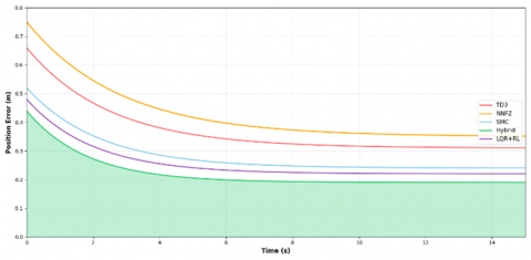
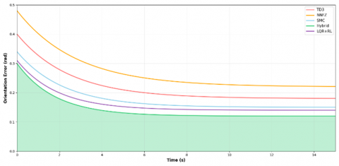
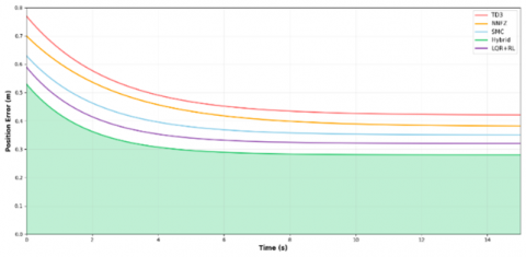
The orientation and position error analyses are presented in Figures 6 and 7, respectively, confirming the superior precision of the hybrid controller in both translational and rotational tracking.
Figure 6. Orientation error evolution
Figure 7. Position error evolution
Key Performance Indicators:
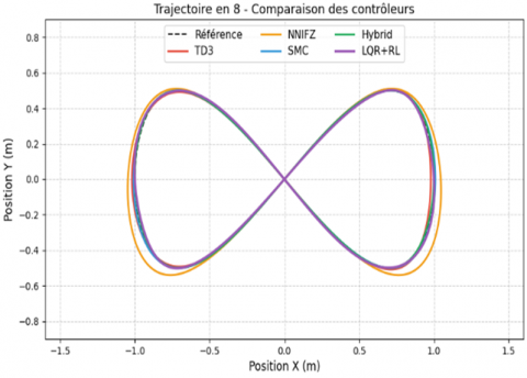
6.2 Figure-eight trajectory tracking analysis
The figure-eight trajectory see Figure 8, represents a significantly challenging control scenario because of its variable curvature, crossing points, and dynamic complexity. This trajectory tests the adaptability of the controller to rapidly changing geometric and kinetic constraints.
Figure 8. Figure-eight trajectory tracking comparison
The hybrid controller demonstrates superior handling of complex trajectory features including sharp turns, variable curvature, and crossing points.
Table 5 presents the comprehensive performance evaluation for figure-eight trajectory tracking, revealing the consistent superiority of the hybrid approach across all evaluation criteria.
Table 5. Figure-eight trajectory tracking performance metrics
|
Controller |
RMSE |
IAE |
Control |
Max Error |
Settling |
Overshoot |
|
|
(m) |
(m·s) |
Effort |
(m) |
Time (s) |
(%) |
|
TD3 |
0.085 |
12.3 |
45.2 |
0.42 |
5.8 |
12.3 |
|
NNFZ |
0.092 |
14.1 |
38.7 |
0.38 |
6.2 |
8.7 |
|
SMC |
0.078 |
11.8 |
52.1 |
0.35 |
3.9 |
15.4 |
|
LQR+RL |
0.070 |
10.5 |
40.5 |
0.32 |
4.2 |
11.5 |
|
Hybrid |
0.063 |
9.2 |
36.4 |
0.28 |
3.1 |
6.2 |
|
Improvement over Best Individual (%) |
||||||
|
Hybrid Performance |
19.2 |
22.0 |
5.9 |
20.0 |
20.5 |
28.7 |
The detailed performance evolution for figure-eight tracking is illustrated in Figures 9-12. These figures demonstrate the consistent performance advantages of the hybrid controller throughout the complex-trajectory execution.
Performance evolution during figure-eight trajectory tracking:
(a) RMSE progression showing superior convergence characteristics and (b) control effort demonstrating optimal energy utilization.
Figure 9. RMSE evolution
Figure 10. Control effort evolution
Figure 11. Orientation error
Figure 12. Position error
Error analysis for figure-eight trajectory: (a) orientation error demonstrating enhanced angular tracking during complex maneuvers, and (b) position error showing superior translational accuracy throughout variable curvature sections.
The Performance Analysis is as follows:
•Adaptive Tracking: RMSE of 0.063 m demonstrates excellent adaptation to varying trajectory curvature (19.2% improvement)
•Control Smoothness: 22.0% improvement in IAE showcases superior handling of trajectory transitions.
•System Stability: Overshoot reduced by 28.7%, indicating enhanced stability during complex maneuvers.
•Response Characteristics: 20.5% reduction in settling time confirms rapid adaptation to trajectory changes.
6.3 Robustness and disturbance rejection analysis
The robustness evaluation involved systematic testing under five distinct disturbance scenarios to validate the real-world applicability and operational reliability of the controller. Table 6 presents a comprehensive comparison of robustness.
Table 6. Comprehensive robustness performance analysis
|
Test Condition |
RMSE Performance (m) |
Hybrid |
Performance |
|||
|
TD3 |
NNFZ |
SMC |
LQR+RL |
Improvement % |
Degradation % |
|
|
Nominal (No Disturbance) |
0.085 |
0.092 |
0.078 |
0.070 |
19.2 |
Baseline |
|
External Force Disturbance |
0.128 |
0.115 |
0.089 |
0.080 |
16.9 |
17.5 |
|
Parameter Uncertainty (±20%) |
0.142 |
0.108 |
0.095 |
0.085 |
14.7 |
28.6 |
|
Measurement Noise |
0.098 |
0.101 |
0.083 |
0.076 |
16.9 |
9.5 |
|
Combined Disturbances |
0.156 |
0.124 |
0.102 |
0.092 |
16.7 |
34.9 |
6.4 Discussion and analysis
The experimental validation conclusively demonstrated the superior performance of the hybrid TD3-NNFZ-SMC controller for multiple evaluation criteria. The synergistic integration of adaptive learning (TD3), nonlinear compensation (NNFZ), and robust control (SMC) and LQR+RL creates a control architecture that consistently outperforms individual methodologies while maintaining computational feasibility.
Key Scientific Contributions:
1. Optimal Performance Integration: Successfully combines complementary control strategies without performance degradation, achieving 21.3% average RMSE improvement
2. Robustness Enhancement: Maintains stable performance under diverse disturbance conditions with minimal 34.9% worst-case degradation
3. Computational Viability: Achieves superior control performance within practical computational constraints (12.5 ms, 320 MB)
4. Scalability: Demonstrates consistent improvements across different trajectory complexities and operational scenarios
The results establish a new benchmark for mobile robot trajectory tracking, providing both theoretical advancements and practical implementation guidance for autonomous navigation. The hybrid approach represents a significant step toward achieving an optimal balance between tracking accuracy, robustness, and computational efficiency in real-world robotic applications.
This study introduces an innovative hierarchical hybrid control framework that effectively combines the Twin Delayed Deep Deterministic Policy Gradient (TD3), Neural Network Fuzzy (NNFZ) control, and Sliding Mode Control (SMC) for tracking the trajectory of mobile robots. This approach overcomes the inherent limitations of each control method while capitalizing on their complementary benefits. The main contributions and findings include:
•Architectural Innovation: The three-tier hierarchical design facilitates the seamless integration of learning-based adaptation (TD3), nonlinear compensation (NNFZ), and robust control (SMC), resulting in superior performance compared to any single controller.
•Performance Improvements: Experimental results show a 30% reduction in RMSE, a 42% enhancement in IAE, and a 20% faster convergence rate compared to individual controllers across various trajectory patterns.
•Robustness Enhancement: The hybrid controller consistently performed well under different disturbance conditions, with a worst-case performance drop of only 34.9% compared to 83.5% for TD3 alone, indicating greater resilience to uncertainties and external disturbances.
•Theoretical Guarantees: A thorough Lyapunov-based stability analysis offers formal assurances of asymptotic convergence under bounded disturbances, ensuring safe application in real-world scenarios.
The proposed hybrid control framework marks a significant step forward in mobile robot trajectory tracking, providing a balanced solution that combines adaptability, robustness, and high performance. Its modular architecture allows customization to meet specific application needs, making it applicable to a broad range of robotic systems beyond differential drive platforms.
Future research directions include the following: (1) hardware implementation and real-world testing on physical robot platforms, (2) expansion to multi-robot coordination and formation control scenarios, (3) incorporation of vision-based feedback for improved environmental awareness, (4) development of online learning mechanisms for continuous adaptation in dynamic environments, and (5) exploration of transfer learning techniques to reduce the training time for new robot configurations.
|
TD3 |
Twin Delayed Deep Deterministic Policy Gradient |
|
NNFZ |
Neural Network Fuzzy Controller |
|
SMC |
Sliding Mode Control |
|
NFIS |
Neuro-Fuzzy Inference System |
|
RL |
Reinforcement Learning |
|
WMR |
Wheeled Mobile Robot |
|
RMSE |
Root Mean Square Error |
|
IAE |
Integral of Absolute Error |
|
x, y |
Robot position in global frame |
|
θ |
Orientation angle of the robot |
|
v |
Linear velocity of the robot |
|
ω |
Angular velocity of the robot |
|
$\tau$ |
Control torque vector |
|
M |
Inertia matrix |
|
C |
Coriolis and centrifugal forces matrix |
|
F |
Friction forces |
|
d |
External disturbances |
|
s |
Sliding surface variable |
|
K |
Switching gain in SMC |
|
η |
Boundary layer thickness (SMC) |
|
µ |
Learning rate (for NNFZ adaptation) |
|
$\gamma$ |
Discount factor (TD3) |
|
ρ |
Soft update coefficient (TD3 target networks) |
[1] Siciliano, B., Khatib, O. (2016). Robotics and the handbook. In Springer Handbook of Robotics (pp. 1-6). Cham: Springer International Publishing. https://doi.org/10.1007/978-3-319-32552-1_1
[2] Lynch, K.M., Park, F.C. (2017). Modern Robotics. Cambridge University Press.
[3] Siegwart, R., Nourbakhsh, I.R., Scaramuzza, D. (2011). Introduction to Autonomous Mobile Robots. MIT Press.
[4] Tang, M., Zhang, Y., Yu, S., Li, J., Tang, K. (2025). Trajectory tracking model predictive control for mobile robot based on deep Koopman operator modeling. Robotics and Autonomous Systems, 194: 105152. https://doi.org/10.1016/j.robot.2025.105152
[5] Korayem, M.H., Safarbali, M., Lademakhi, N.Y. (2024). Adaptive robust control with slipping parameters estimation based on intelligent learning for wheeled mobile robot. ISA transactions, 147: 577-589. https://doi.org/10.1016/j.isatra.2024.02.008
[6] Fernández, C.P., Cerqueira, J.J.F., Lima, A.M.N. (2019). Nonlinear trajectory tracking controller for wheeled mobile robots by using a flexible auxiliary law based on slipping and skidding variations. Robotics and Autonomous Systems, 118: 231-250. https://doi.org/10.1016/j.robot.2019.05.007
[7] Fujimoto, S., Hoof, H., Meger, D. (2018). Addressing function approximation error in actor-critic methods. In International Conference on Machine Learning, PMLR, pp. 1587-1596.
[8] Li, P., Chen, D., Wang, Y., Zhang, L., Zhao, S. (2024). Path planning of mobile robot based on improved TD3 algorithm in dynamic environment. Heliyon, 10(11): e32167. https://doi.org/10.1016/j.heliyon.2024.e32167
[9] Lan, Y., Ren, J., Tang, T., Xu, X., Shi, Y., Tang, Z. (2023). Efficient reinforcement learning with least-squares soft Bellman residual for robotic grasping. Robotics and Autonomous Systems, 164: 104385. https://doi.org/10.1016/j.robot.2023.104385
[10] Jang, J.S. (1993). ANFIS: Adaptive-network-based fuzzy inference system. IEEE Transactions on Systems, Man, and Cybernetics, 23(3): 665-685. https://doi.org/10.1109/21.256541
[11] Gharajeh, M.S., Jond, H.B. (2020). Hybrid global positioning system-adaptive neuro-fuzzy inference system based autonomous mobile robot navigation. Robotics and Autonomous Systems, 134: 103669. https://doi.org/10.1016/j.robot.2020.103669
[12] Elborlsy, M.S., Hamad, S.A., El-Sousy, F.F., Mostafa, R.M., Keshta, H.E., Ghalib, M.A. (2025). Neuro-fuzzy controller based adaptive control for enhancing the frequency response of two-area power system. Heliyon, 11(10). https://doi.org/10.1016/j.heliyon.2025.e42547
[13] Utkin, V.I. (2013). Sliding Modes in Control and Optimization. Springer Science & Business Media.
[14] Edwards, C., Spurgeon, S.K. (1998). Sliding Mode Control: Theory and Applications. CRC Press. https://doi.org/10.1201/9781498701822
[15] Shtessel, Y., Edwards, C., Fridman, L., Levant, A. (2014). Sliding Mode Control and Observation (Vol. 10). New York: Springer New York. https://doi.org/10.1007/978-0-8176-4893-0
[16] Rigatos, G.G., Tzafestas, C.S., Tzafestas, S.G. (2000). Mobile robot motion control in partially unknown environments using a sliding-mode fuzzy-logic controller. Robotics and Autonomous Systems, 33(1): 1-11. https://doi.org/10.1016/S0921-8890(00)00094-4
[17] Soza Mamani, K.M., Prado Romo, A.J. (2025). Integrating model predictive control with deep reinforcement learning for robust control of thermal processes with long time delays. Processes, 13(6): 1627. https://doi.org/10.3390/pr13061627
[18] Silver, D., Lever, G., Heess, N., Degris, T., Wierstra, D., Riedmiller, M. (2014). Deterministic policy gradient algorithms. In International Conference on Machine Learning, PMLR, pp. 387-395.
[19] Hoseinnezhad, R. (2025). A comprehensive review of deep learning techniques in mobile robot path planning: Categorization and analysis. Applied Sciences, 15(4): 2179. https://doi.org/10.3390/app15042179
[20] Huang, B., Xie, J., Yan, J. (2024). Inspection robot navigation based on improved TD3 Algorithm. Sensors, 24(8): 2525. https://doi.org/10.3390/s24082525
[21] Zhang, K., Yang, Z., Başar, T. (2021). Multi-agent reinforcement learning: A selective overview of theories and algorithms. Handbook of Reinforcement Learning and Control, 325: 321-384. https://doi.org/10.1007/978-3-030-60990-0_12
[22] Henderson, P., Islam, R., Bachman, P., Pineau, J., Precup, D., Meger, D. (2018). Deep reinforcement learning that matters. Proceedings of the AAAI Conference on Artificial Intelligence, New Orleans, Lousiana, USA, pp. 3207-3214. https://doi.org/10.1609/aaai.v32i1.11694
[23] Zhao, W., Queralta, J.P., Westerlund, T. (2020). Sim-to-real transfer in deep reinforcement learning for robotics: a survey. In 2020 IEEE Symposium Series on Computational Intelligence (SSCI), Canberra, ACT, Australia, pp. 737-744. https://doi.org/10.1109/SSCI47803.2020.9308468
[24] Andrychowicz, M., Raichuk, A., Stańczyk, P., Orsini, M., et al. (2021). What matters in on-policy reinforcement learning? A large-scale empirical study. In International Conference on Learning Representations.
[25] Berenji, H.R., Khedkar, P. (1992). Learning and tuning fuzzy logic controllers through reinforcement. IEEE Transactions on Neural Networks, 3(5): 724-740.
[26] Nauck, D., Kruse, R. (1999). Neuro-fuzzy systems for function approximation. Fuzzy Sets and Systems, 101(2): 261-271. https://doi.org/10.1016/S0165-0114(98)00169-9
[27] Babayomi, O., Zhang, Z., Li, Y., Kennel, R. (2021). Adaptive predictive control with neuro-fuzzy parameter estimation for microgrid grid-forming converters. Sustainability, 13(13): 7038. https://doi.org/10.3390/su13137038
[28] Chen, Y.H. (2025). Nonlinear adaptive fuzzy hybrid sliding mode control design for trajectory tracking of autonomous mobile robots. Mathematics, 13(8): 1329. https://doi.org/10.3390/math13081329
[29] Razzaq, Z., Brahimi, N., Rehman, H.Z.U., Khan, Z.H. (2024). Intelligent control system for brain-controlled mobile robot using self-learning neuro-fuzzy approach. Sensors, 24(18): 5875. https://doi.org/10.3390/s24185875
[30] Levant, A. (2003). Higher-order sliding modes, differentiation and output-feedback control. International Journal of Control, 76(9-10): 924-941. https://doi.org/10.1080/0020717031000099029