Almojtaba Munaf*![]() | Ahmed Rahman Jasim Almusawi
| Ahmed Rahman Jasim Almusawi![]()
© 2025 The authors. This article is published by IIETA and is licensed under the CC BY 4.0 license (http://creativecommons.org/licenses/by/4.0/).
OPEN ACCESS
In the robotics field, with the rapid development of robotics, the challenge of devising effective strategies for planning paths for mobile robots navigating unfamiliar terrain has become increasingly central, impacting a wide range of industrial and academic applications. This research addresses the application of the Q-learning algorithm to construct a mathematical model of a differentially driven mobile robot. The algorithm enables the robot to independently control and execute four kinematic actions-up, down, right, and left-thus determining its path in unpredictable, constrained environments through an experimental and systematic approach. Our research focuses on using Q-learning to enable trajectory generation for differentially driven mobile robots, allowing them to navigate autonomously and skillfully adapt to their environment. Simulation results demonstrate that Q-learning achieves significantly higher computational efficiency, reducing computation time from 0.37 s with MPC to 0.22 s in simple maps (a 40% improvement) and from 3.74 s to 0.875 s in complex maps (a 75% improvement). In terms of path planning, Q-learning achieved a shorter trajectory in simple environments (51 units vs. 73.61 units with MPC), while in highly complex terrains it successfully reached the goal with longer but safer paths (163.57 units vs. 76 units with MPC), ensuring robust obstacle avoidance. Although Q-learning required more iterations to converge (250 vs. 3 with MPC), it consistently adapted to dynamic environments where MPC performance deteriorated. These results confirm that Q-learning not only outperforms MPC in convergence speed and path optimization under uncertainty but also enhances navigation efficiency in dynamically changing environments. The insights derived from this study highlight the transformative potential of reinforcement learning in mobile robotics, paving the way for future innovations in autonomous navigation.
machine learning, Q-learning, path planning (PP), differential-drive robotics (DDR), mobile robot path planning (MRPP), trajectory tracking, reinforcement learning, autonomous navigation, obstacle avoidance
The integration of “ML” strategies into the realm of robotics has opened new avenues for addressing complex challenges, specially inside the area of trajectory monitoring for robots. These improvements are vital given the robots' giant programs inside the agriculture industry, surveillance, among others [1]. Robots work to reduce labor, reduce costs, save time and increase human life by increasing efficiency. His deployment in many applications highlights his versatility and power for power. Navigating and progress from visible features in many environments from indoor space to robust landscape [2]. A mobile robot is defined as an independent entity designed to navigate and maneuver thru various environments. Equipped with mobility mechanisms inclusive of wheels, tracks, and legs, these robots can navigate through a large number of terrains. Their functionality to function in a huge choice of settings, from indoor facilities to rugged out of doors landscapes, underscores their versatility and importance in pushing the bounds of robotics era and tackling difficult demanding conditions presented via diverse environments. Central to leveraging this versatility for realistic applications is the robotics functionality for powerful trajectory monitoring control [3]. Trajectory-tracking control for a (MR) involves ensuring that the robotics’ modern-day position and orientation converge toward a predetermined reference course. This path can be predefined or generated dynamically, along with following the trajectory of a shifting digital target. The elementary aim is to manual the mobile robotic successfully alongside the required trajectory. Path planning as a consequence constitutes a critical computational challenge in the subject of robotics, representing a critical and integral talent [4]. The primary objective of path planning is to identify the gold standard route between a place to begin and a destination. In the context of most robots, achieving optimal path planning typically entails determining the shortest distance between two locations [5]. This fundamental aspect of robotics not only underscores the complexity of navigating through unpredictable terrains but also highlights the necessity for progressive solutions that could dynamically adapt to new environments. Machine learning for mobile robots refers to the usage of system mastering techniques and algorithms along with reinforcement learning (RL), neural networks, supervised learning, imitation learning, planning and optimization, Bayesian Filters, and Monte Carlo methods that are used to enable autonomous or semi- autonomous robots to perceive, navigate, and have interaction with their environment [6]. This study is dedicated to harnessing system studying strategies for reinforcing path planning in mobile robots. At its core, this research develops and trains a mathematical version utilizing the Q-learning set of rules for a differential power robot. Q-L algorithm for a differential drive robot. Q-L essence resides in its trial-and-error process, empowering the robot to autonomously identify the most efficient path across unknown terrains [7]. Through analytical comparison, Q-learning has performed better performance Methods of traditional trajectory planning, fast navigation, characterized by small routes and high precision Obstacle. These findings confirm the extraordinary ability of Q learning in the selection of refining Offer a significant advantage to navigate through an unwanted environment without the need for pre-existing maps or knowledge. The basic aim of this paper is to explore the demanding situations of course making plans in undefined environments and to propose a novel approach the use of device getting to know to decorate the adaptability and performance of cellular robots. By leveraging the strengths of Q-learning, this research now not best addresses the inherent barriers of traditional direction planning strategies but also units a brand-new benchmark for self-sufficient navigation. The primary problem addressed in this research is the task of skilled track plan for cell robots. Navigate unwanted and dynamically converted environment. Traditional methods such as model predictive Control (MPC) often decreases because of their dependence on predefined models and limited adaptability unexpected boundaries. The purpose of this research is to monitor the path and increase the direction. The ability to plan mobile robots by taking advantage of the Q-learning algorithm. The purpose of this research is to develop A strong machine learning -based structure that allows the medium -differential-drive robots to be autonomously Navigate through complex areas with speeds of progress and course performance. The approach involves imposing the Q-L algorithm to train a mathematical version of the robotic, putting in place numerous simulated environments to assess performance, and engaging in a comparative analysis with MPC to demonstrate the benefits of Q-L in dynamic and unpredictable settings. Through this research, the test seeks to contribute to the development of autonomous navigation in robotics by addressing the constraints of traditional methods and proposing an extra adaptable and green solution.
The use of Q-learning and Sarsa algorithms for mobile robot path planning was examined in the reference [8]. Through digital experiments, it becomes located that Q-learning is quicker but Sarsa offers more secure paths. The studies aimed to optimize those algorithms for performance and protection through adjusting parameters. While Q-learning is appropriate for velocity-vital responsibilities, Sarsa is most well-known for scenarios requiring caution. The study's limitation lies in its virtual testing environment, which might not fully reflect real-world complexities. A reinforcement learning (RL) algorithm for mobile robot position control in a 3D simulation, aimed at engineering education was introduced in the reference [9]. The algorithm has a learning phase, where it autonomously learns navigation and an operational phase for position control application. Its advantage is model-free autonomous learning, with the main drawback being the long learning time required. Initial results indicate improved target navigation with increased iterations, though not surpassing the integral position control (IPC) algorithm due to velocity adjustment limitations. Future efforts will focus on incorporating linear velocity and distance learning to improve the model's performance for educational use with actual robots. Multi-robot path planning was focused on in the reference [10], a novel approach using deep Q-network (DQN), was introduced, the proposed method employs DQN to train a policy network, mapping environmental states to actions. Leveraging neural networks and hierarchical reinforcement learning (HRL) for autonomous path planning in mobile robots was focused on in the reference [11].
These techniques address limitations in existing robots, enhancing adaptability to changing environments and improving convergence rates. A navigation technique for mobile robots combining deep reinforcement learning and recurrent neural networks was developed in the reference [12], improving pathfinding in diverse environments. Tests confirm its effectiveness in optimizing path efficiency and reducing lengths. Future work will tackle more complex scenarios. A method that combines the double deep Q-network (DDQN) algorithm was proposed in the reference [13], which addresses the overestimation problem inherent in deep Q-network (DQN), with an RNN module to capture temporal dependencies in the robot's environment. A deep reinforcement learning (DRL) method for guiding nonholonomic wheeled mobile robots (NWMRs) for path-following and avoiding obstacles was presented in the study [14], utilizing the deep deterministic policy gradient (DDPG) algorithm. Unlike traditional methods, this DRL approach can handle continuous control challenges without pre-existing dynamic models. The approach introduces an efficient manipulation technique for path navigation and obstacle evasion, optimizing kingdom and reward talents for complicated environments. Through simulations, the technique proves superior to traditional version predictive control (MPC), showcasing better path adherence and impediment negotiation with extra fine accuracy and robustness. These paintings advance the combination of DRL in robotic navigation, paving the manner for greater adaptable and smart self-sustaining structures. A deep reinforcement learning method for rapid trajectory planning and control of mobile robots in unknown environments was introduced in the reference [15]. Despite promising consequences, further investigation is wanted to assess robustness and scalability throughout various settings. A reinforcement learning (RL) approach for controlling robots with mecanum wheels was introduced in the study [16], enabling omnidirectional movement. Unlike conventional control structures that require exact robotic fashions, RL learns immediately from environmental interactions, addressing version uncertainties and nonlinearities. The study develops a unique reward characteristic tailor-made for mecanum-wheeled robots, facilitating navigation toward a goal at the same time as retaining orientation. Simulations display the effectiveness of the proposed RL approach, suggesting its capability for complicated robot manage responsibilities. Future paintings might also discover extra superior navigation challenges for mecanum-wheeled robots.
A smart cleaner mobile robot avoiding obstacles is designed to clean the building’s flat and complex ground and it is too useful to reduce the time and effort’s person in the cleaning process. The proposed device included: the forward and inverse kinematics is derived to compute an accurate position and orientation for complex states of the mobile robot [17].
In this research, Q-L is used to educate a mathematically model of a DDMR to get its route using some unknown maps in special eventualities.
3.1 Q-learning algorithm
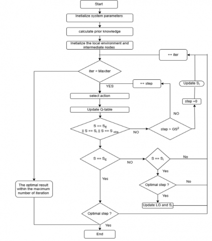
Q-L is a reinforcement learning approach for fashions to iteratively improve by way of selecting optimal moves. It operates without a pre-defined version of the environment, mastering from moves' consequences-rewards for desirable movements and consequences for undesirable ones. Through non-stop interplay and exploration of the surroundings, the "agent" autonomously predicts and adapts. This method includes adjusting strategies based on exploration effects and enhancing decision-making over time. The learning process of the Q-learning algorithm is outlined in Algorithm 1 and illustrated in Figure 1. The updating process is described mathematically in Eq. (1).
Figure 1. Q-learning flowchart
The multiple additives of Q-L include:
Agent: This is an entity that operates inside an environment and exhibits movement.
States: This variable denotes the present position of an agent inside an environment.
Actions: It elucidates the functions or actions executed by the agent while situated in a particular place within an environment.
Rewards: This reinforcement establishes a fundamental idea in the learning environment, where the agent receives either positive or negative feedback based on the characteristics.
Episodes: When an agent reaches a juncture at which he can no longer accept additional tasks, resulting in the conclusion of an episode.
The Q value: a calculation that determines the usefulness or efficiency of an action. in a certain setting in the context of learning a reinforcement.
Belman's equation: a recurrent system used to make best decisions. In Q-L, this equation is used to determine a specific state fee and evaluate its relatives. Help with status adaptability and decision-making.
3.1.1 Reward function design
The performance of reinforcement learning algorithms is highly dependent on the reward function, which defines the objective for the agent. In this study, the reward function was designed to balance three main goals: (i) reaching the target as efficiently as possible, (ii) avoiding collisions with obstacles, and (iii) minimizing unnecessary exploration. The design of the reward function is a key element for reinforcement learning. The positive and negative reward structure ensures convergence. The reward values were defined as follows:
•Goal reached: + 100
•Provides a strong incentive to complete the task successfully. A high positive reward ensures that the agent prioritizes reaching the goal state above all other actions.
•Collision with obstacle: - 100
•Introduces a strong penalty to discourage unsafe trajectories. The large negative reward makes obstacle avoidance a primary behavior.
•Step penalty: -1 per action
•Encourages the agent to minimize path length and avoid wandering, as each unnecessary step reduces the cumulative reward.
3.1.2 Theoretical basis
•According to reinforcement learning theory [7], a sparse but high terminal reward (goal) combined with dense intermediate penalties (steps, collisions) accelerates convergence by shaping the exploration space.
•The choice of +100 and -100 maintains symmetry, ensuring the agent evaluates reaching the goal and avoiding failure as equally critical.
3.2 Path-planning using Q-L
The fundamental concept of the QL-based path planning method is centered on the Q-learning algorithm. In this approach, the Q-value associated with each state-action pair is updated during the learning process, this method incorporates the Q value of the subsequent state-action pair generated by the policy being evaluated, under the current policy, rather than the Q value of the subsequent state-action pairings. In mobile robot path planning, the algorithm operates by randomly sampling the environment and generating potential paths over multiple iterations. During this process, the behavior policy interacts with the target policy progressively adapts, converging toward the optimal path. The fundamental concept behind the QL-based totally route making plans approach entails the Q-L set of rules. When revising the Q value of a state-action pair, this approach includes the Q value of the following state action pair generated with the aid of the coverage below assessment, as opposed to the Q-value of the next state-action pair adhering to the cutting-edge policy. Consider planning the course. The algorithm for cellular robots requires random sampling samples and producing them over a number of samplings tries. Throughout this process, the interplay between behavioral policy and objectives consistently ensures the attainment of the most lucrative route. The learning method of the Q-L algorithm is outlined in Algorithm 1 and Figure 1. The updating process described by Eq. (1) unfolds as follows [18]:
$Q(s, a)=Q(s, a)+\alpha\left[r+\gamma \cdot a^{\prime} \max Q\left(s^{\prime}, a^{\prime}\right)-Q(s, a)\right]$ (1)
where, $s, \mathrm{a}, r$ and $s^{\prime}$ represent state, action, the reward received as a reinforcement signal after executing action $s$ and next state respectively, $\gamma(0 \leq \gamma<1)$ is discount factor, and $\alpha(0 \leq \alpha<1)$ is learning rate. Various approaches have been used to tackle the issues.
3.2.1 Hyperparameter settings for Q-learning
In our experiments, the Q-learning algorithm was trained using the following hyperparameters:
•Learning rate ($\alpha$): 0.1
•Chosen to ensure stable but reasonably fast convergence without overshooting.
•Discount factor ($\gamma$): 0.9
•Balances immediate rewards with long-term gains, suitable for navigation tasks where reaching the goal is critical.
•Exploration rate ($\varepsilon$): Initially set to 1.0 and decayed linearly to 0.1 over 200 episodes.
•Ensures sufficient exploration in the early stage and exploitation in later stages.
•Number of episodes: 250 (consistent with the iteration counts in the results).
|
Algorithm 1. Q-learning algorithm [19] |
|
1. Preamble $\mathrm{Q}_{\mathrm{n} \times \mathrm{m}}(\mathrm{s}, \mathrm{a})=0$ for all $n$ states and $m$ actions. 2. Recur 3. Use $\varepsilon$-greedy strategy to choose action a from the current states; 4. Execute action a, receive reward r, and observe new ${states}^{\prime}$. 5. Update Q-value: apply Eq. (1) to update Q (s, a). 6. Set $\mathrm{s} \leftarrow \mathrm{s}^{\prime}$ 7. Until the state ‘s’ reaches the destination |
3.3 Simulation environment and robot model
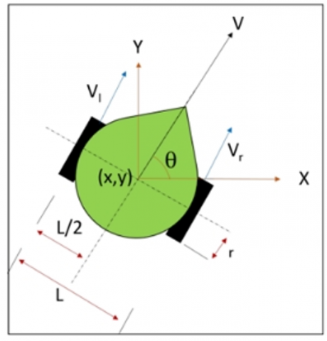
To simulate the differential-drive mobile robot (DDMR), the differential-drive library in Python was used. The robot kinematics are described in Eqs. (2)-(7). The structure of the robot is shown in Figure 2. This library enables accurate modeling of the robot's kinematics and physical behavior by incorporating essential mechanical parameters such as wheel radius and wheel base. The robot's motion was not simulated as a simple grid movement but rather as continuous pose updates in two-dimensional space, considering the robot’s heading angle (θ), linear and angular velocities. The forward kinematics were calculated based on the velocity of the left and right wheels (Vl and Vr), and the robot’s updated pose (x, y, θ) was determined using differential drive motion Eqs. These calculations reflect the real physical constraints and behavior of an actual mobile robot. Using this model, the Q-learning algorithm was implemented to control the robot’s movements (up, down, right, left) in response to the environment. The learning process was guided by a reward function designed to encourage reaching the goal while avoiding obstacles. The use of the differential-drive model provides a realistic and physically- grounded environment, bridging the gap between theoretical learning algorithms and practical robotic applications.
Figure 2. Differential drive mobile robot [20]
3.4 Differential drive
The MR platform illustrated in Figure 2 features two driving wheels arranged side by side, along with a single passive wheel designed to maintain the robot's static stability. The radius of driving wheels is denoted as "r", while "L" represents the distance among the two wheels, enabling the robot to travel from one point to another, understanding its position and direction is crucial; it needs to be aware of both its location and the way it is facing to navigate from one place to another [19].
By separating the velocities of each wheel, the path can be replaced by the robot. Assume the rotation speed ($\omega$) around the instantaneous curvature center (ICC) must be the same for both wheels, which can be expressed by the following equations.
$V r=\omega\left(R+\frac{1}{2}\right)$ (2)
$V r=\omega\left(R-\frac{1}{2}\right)$ (3)
where, R: is the signed distance from the ICC to the midpoint between the wheels.
Vr and Vl represent the Velvet of the right and left wheels respectively on the ground., and ICC: At any instant, point R represents the center of curvature and $\omega$ can be solved as follows:
$R=\frac{l}{2} \frac{(V l+V r)}{V r-V l}$ (4)
$\omega=\frac{(V r+V l)}{l}$ (5)
when Vl = Vr the robot moves in a straight line with linear motion.
If Vl = - Vr then R = 0 resulting in rotation about the midpoint of the wheel axis - a rotation in place occurs. Should Vl = 0 the robot will rotate around the left wheel, with R = - l/2. The same principle applies if Vr = 0, R = l/2 [21].
3.5 Forward kinematics for differential drive robots
In Figure 2, it is considered that the robot is positioned at coordinates (x, y) and oriented in a direction defined by an angle θ relative to the x-axis. It is assumed that the robot's center coincides with a point along the wheel axle. Through the manipulation of control parameters Vl and Vr, the robot can be maneuvered to various positions and orientations. The control parameters Vl and Vr are understood to represent the velocities of the “L” and “R” wheels influence the robot's movement and direction. Once the velocities Vl and Vr are known, the ICC location can be calculated using Eq. (3). Which determined as follows:
$I C C=[X-R \sin (\theta), y+R \cos (\theta)]$ (6)
and at time t + $\delta$t the robot’s pose will be:
$\begin{gathered}{\left[\begin{array}{c}x^{\prime} \\ y^{\prime} \\ \theta\end{array}\right]=\left[\begin{array}{ccc}\cos (\omega \delta t) & -\sin (\omega \delta t) & 0 \\ \sin (\omega \delta t) & \cos (\omega \delta t) 0 & 0 \\ 0 & 0 & 1\end{array}\right]+} {\left[\begin{array}{c}x-I C C x \\ y-I C C y \\ \theta\end{array}\right]+\left[\begin{array}{c}I C C x \\ I C C y \\ \omega \delta t\end{array}\right]}\end{gathered}$ (7)
This Eq. (7) simply describes the motion of a robot rotation (R) about its ICC with an angular velocity of ω [22].
Regarding to the significance of path planning and control of robot, it plays a crucial role in various industries and fundamental applications in life, especially considering the rapid advancements witnessed globally and the desire to simplify human life by exploring alternatives that provide accurate results in a short time and at a lower cost. This research focuses on studying a mathematical model for a “DDMR” using the Q-L algorithm. The algorithm incorporates the application of the Bellman Eq., chosen for its ability to run without prior knowledge of the robot's surroundings. It trains the robot through trial-and-error techniques, introducing four possible movements for the robot (up, down, right, left), representing the actions in Q-L. The aim of this work is analyzing the state and clarify how the robot selects its path, subsequently comparing the results with the model predictive control algorithm.
4.1 Training D using Q-L algorithm
As shown in Eq. (1), to train the robot, four possible actions were defined (up, down, right, left). The learned Q-values for selected points are summarized in Table 1. These movements can vary based on the robot's state, depending on the presence or absence of obstacles in the map. The aim is to find the best path for the robot, considering the changing movements, by identifying the shortest possible route that can be reached in the least amount of time. This is achieved by adapting to the robot's requirements, considering the presence of obstacles in the environment. To implement this training, the differential drive library in Python was utilized.
Table 1. Q-values for each action in selected states (corresponding to Figure 8)
|
Point |
Action 0 (Up) |
Action 1 (Down) |
Action 2 (Right) |
Action 3 (Left) |
|
(5, 5) |
-7.1428 |
-7.1428 |
-7.1428 |
-7.1428 |
|
(10,10) |
-7.1428 |
-7.1428 |
-7.1428 |
-7.1428 |
|
(15, 15) |
-7.1427 |
-7.1427 |
-7.1427 |
-7.14276 |
|
(25, 25) |
-7.1423 |
-7.1424 |
-7.1423 |
-7.1423 |
|
(35,35) |
-5.7936 |
-6.8712 |
-6.9026 |
-6.8622 |
|
(45,45) |
20.4279 |
30.1351 |
20.4279 |
30.1351 |
For the point (5,5) the negative values indicate that the agent should avoid these actions at this state. The closer the value is to zero, the better the action is perceived. For the point (10,10) similar to the previous point, these negative values suggest that the agent should avoid these actions at this state. For the point (15,15) The agent prefers moving down (action 1) or left (action 3) at this state as these have relatively higher Q-values. For the point (25,25) The agent shows a preference for moving left (action 3) as it has the highest Q-value. For the point (35,35) The agent seems to have updated its preference at this state, and the Q-values indicate a higher value for moving left (action 3) compared to the previous results. For the point (45,45) The positive values indicate a high preference for moving down (action 1) or left (action 3) at this goal state, suggesting a favorable path towards the goal with a high reward.
4.2 Environment configuration for algorithm evaluation
The efficacy of path planning algorithms, such as Q-learning and model predictive control (MPC), is profoundly influenced by the complexity and nature of the environment in which they operate. To systematically assess these algorithms' performance, this study employs a series of simulated environments, each designed to incrementally increase complexity. These environments simulate realistic scenarios that a mobile robot may encounter, ranging from open spaces to densely populated obstacle fields. The evaluation was carried out in six environment models. The results of these environments are presented in Table 2 and illustrated in Figures 3-7.
Table 2. Average performance parameters of Q-learning
|
Parameters |
First Map |
Second Map |
Third Map |
Fourth Map |
Fifth Map |
Sixth Map |
|
Computation time |
0.35 (s) |
1.4(s) |
1.52 (s) |
01.85 (s) |
1.625(s) |
1.125(s) |
|
Path length |
103 |
135 |
115 |
129 |
156 |
163 |
|
Iterations |
250 |
250 |
250 |
250 |
250 |
250 |
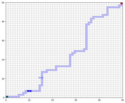
Figure 3. Navigation of the differential-drive mobile robot in an open environment without obstacles
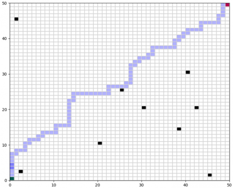
Figure 4. Q-learning trajectory in an environment with randomly distributed obstacles
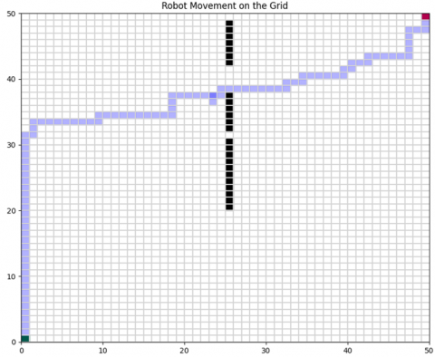
Figure 5. Robot trajectory in a linear obstacle scenario
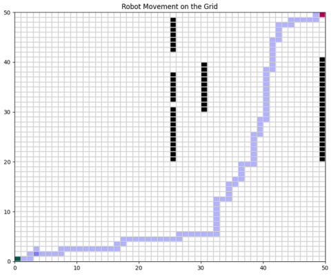
Figure 6. Navigation in a complex terrain with multiple obstacles
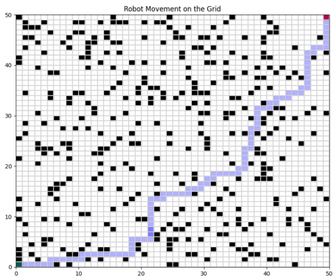
Figure 7. Path planning performance in a high-density obstacle environment
In Figure 3, the robot follows the shortest trajectory toward the goal.
The plot in Figure 4 shows how the robot adapts its path to avoid collions.
In Figure 5, the robot successfully plans a path around the barrier to reach the goal position.
In this Figure 6, the Q-learning agent adjusts its trajectory to avoid clustered obstacles.
In this Figure 7 the longer path reflects safe navigation around all barriers.
4.2.1 Environment models
Model 1: Basic navigation scenario
•Description: This initial model presents a straight route with a straight route
The beginning of the target point, devoid of obstacles. It acts as a goal to assess the origin
The navigation effect of the algorithm.
•Objective: Evaluate algorithm efficiency in unobstructed conditions.
Model 2: Random obstacle distribution
•Description: Introduction to randomly, this version simulates an environment with boundaries
• An unexpectedly assigned on the map. It examines the adaptability of the algorithm and dynamic pathfinding capabilities.
•Objective: Assess adaptability to spontaneous environmental changes.
Model 3: Linear obstacle challenge
•Description: A direct barrier between the starting and destination points is presented, challenging the algorithms to navigate around or over linear obstacles efficiently.
•Objective: Examine obstacle negotiation strategies in the presence of direct barriers.
Model 4 & Model 5: Complex Terrains
•Description: These models introduce multiple layers of constraints and more elaborate terrain configurations, representing highly complex environments. The density and arrangement of obstacles are carefully calibrated to simulate real-world navigation challenges.
•Objective: To investigate algorithm performance under high-complexity conditions.
Model 6: High-Density Obstacle Environment
•Description: This model introduces multiple layers of constraints and intricate terrain configurations, representing highly complex environments. The density and distribution of obstacles are meticulously designed to replicate real-world navigation challenges.
•Objective: Evaluate path planning efficiency and obstacle avoidance in dense environments.
4.2.2 Methodological approach
Each environment model changed into meticulously designed to incrementally introduce and strengthen navigation challenges, bearing in mind a complete evaluation of the Q-studying and MPC algorithms across a spectrum of real-global situations. The models range from essential to relatively complicated environments, supplying insights into the algorithms' robustness, adaptability, and performance in dynamic and unpredictable settings.
4.2.3 Analytical framework
The simulated environments serve as controlled framework for systematically reading the overall performance metrics of Q-mastering and MPC algorithms. These metrics consist of computation time, path length, and the range of iterations to reach the designated purpose. The environments facilitate nuanced information about each algorithm's strengths and barriers, informing the improvement of more powerful and adaptable path planning techniques for autonomous cellular robots.
By using this environment simulation-based technique, the study aims to derive empirical evidence of the comparative advantages of study-based path planning strategies, especially Q-learning, against algorithms such as MPC. The insights received from these simulations are anticipated to make contributions drastically to the sector of robotics, particularly in enhancing independent navigation capabilities through the utility of sophisticated machine learning strategies.
The simulation consequences provide a quantifiable assessment of the Q-learning algorithm's performance throughout six unique environmental fashions, each presenting various tiers of complexity and impediment density. The data from Table 2 reveals numerous key insights into the algorithm's path planning efficiency and adaptableness:
Table 3. Environment performance comparison between Q-learning and MPC
|
Map Type |
Simple Map |
Complex Map |
||
|
Parameters |
Q-learning |
Model predictive control |
Q-learning |
Model predictive control |
|
Average iteration |
164 |
15 |
250 |
3 |
|
Computation time (sec.) |
0.22 sec |
0.3733sec |
0.875 sec |
3.744 sec |
|
Average path length |
51.0000 |
73.61 |
163.578 |
76 |
|
Average total step |
8 |
16 |
162 |
3 |
•Performance across environments: The set of rules demonstrated the capability to navigate through environments with increasing complexity, as evidenced via the computation instances which ranged from zero.35 seconds inside the simplest surroundings (first map) to at least one.85 seconds in one of the more complicated environments (fourth map). This variability in computation time underscores the Q-learning adaptability to the surrounding’s complexity.
•Path length optimization: The path lengths, which indicate the efficiency of the route chosen by the algorithm, varied across the scenarios. Notably, the shortest route turned into accomplished in the handiest surroundings (103 units inside the first map), at the same time as the longest course was located in the most complicated surroundings (163 gadgets within the sixth map). This trend shows that as environmental complexity increases, the algorithm strategically opts for longer routes that dodge boundaries, prioritizing successful navigation over path duration minimization.
•Consistent iteration counts: Across all environmental fashions, the new release depends remained regular at 250 iterations. This consistency demonstrates the algorithm's solid performance in phrases of convergence price, no matter the environmental complexity.
•Discussion: The obtained outcomes offer compelling evidence of Q-learning effectiveness in path planning for cell robots, in particular in unknown or dynamically converting environments. Several essential observations may be drawn:
•Adaptability to environmental complexity: Q-learning's performance in environments with random obstacles and complex terrain layouts illustrates its sturdy adaptability. Unlike conventional path planning algorithms which can require pre-defined environmental models, Q-learning method lets in it to dynamically alter its method primarily based on actual-time feedback from the environment.
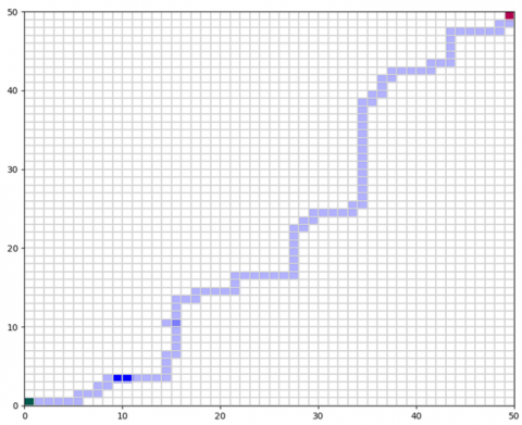
The results demonstrate the efficiency of Q-learning across increasing levels of complexity. The Q-values illustrating convergence in a complex environment are shown in Figure 8. The comparison between Q-learning and MPC is summarized in Table 3 and illustrated in Figures 9-12.
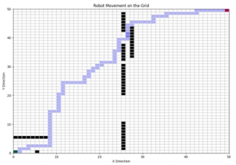
Figure 8. Comparison of Q-learning’s successful trajectory in a complex environment with multiple obstacles
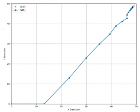
Figure 9. Q-learning adaptability in a complex environment
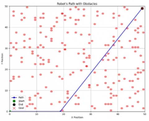
Figure 10. Model predictive control in a simple map: A comparative analysis
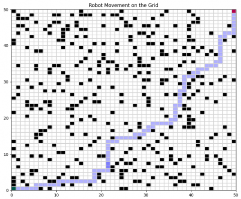
Figure 11. Implementing Q-learning in a highly complex map
Figure 12. Model predictive control in complex terrain
The plotted Q-values indicate convergence toward an optimal safe path.
5.1 Efficiency vs. accuracy trade-off
The variant in path lengths throughout extraordinary fashions highlights an alternate-off between performance and accuracy. In less difficult environments, Q-learning of successfully reveals shorter paths, even as in greater complicated settings, it opts for slightly longer paths to ensure impediment avoidance and aim success. This exchange-off is a vital consideration for real-global packages were navigating safely may outweigh the want for the absolute shortest path.
Implications for Autonomous Robotics: The findings have considerable implications for the improvement of independent robotic systems, mainly in packages requiring navigation in unpredictable or poorly mapped environments. Q-learning's demonstrated ability to learn and adapt in actual time makes it a valuable device for enhancing the autonomy and operational performance of robot.
5.2 Comparing between Q-learning path planning algorithm and model predictive control path planning algorithm
Adaptability:
•Excel in unexpected environment by using your strategy through learning from Q-learning
Interaction, ideal for areas with dynamic changes.
•MPC depends on predefined models, performing well in predicted settings but can tire together
Unexpected changes.
Computational efficiency:
•MPC is precise but computationally intensive in complex scenarios due to optimization over a finite horizon.
•Q-learning potentially offers better long-term efficiency by iteratively improving policy with less immediate computational demand.
Dynamic environment performance:
•Q-learning's model-free approach allows seamless adaptation to changing environments, making it superior in scenarios with frequent alterations.
•MPC's performance is contingent on the accuracy of the environmental model, limiting its adaptability to dynamic changes.
Real-World application:
•Integrating Q-learning in real-world scenarios requires addressing its exploratory time cost.
•MPC necessitates accurate, up-to-date environmental and system dynamics.
•Models, tough in evolving eventualities.
The preference between Q-learning and MPC relies upon at the application's adaptability desires, computational constraints, and environmental dynamics.
•Future research could explore hybrid models that combine Q-learning's adaptability with MPC's precision, aiming for optimized performance across diverse navigation challenges.
In this work, Q-learning and Model Predictive Control (MPC) were applied to the trajectory planning and control of a mobile robot. The results demonstrate that Q-learning provides a flexible and model-free solution, making it particularly suitable for scenarios where the environment is uncertain, dynamic, or difficult to model accurately. On the other hand, MPC showed superior performance in structured environments where an accurate system model is available and computational resources allow real-time optimization. From a practical standpoint, Q-learning is recommended for applications such as autonomous navigation in unknown terrains, exploration tasks, or situations with high variability in operating conditions. Conversely, MPC is more applicable to industrial settings, automated guided vehicles, or environments where constraints and safety requirements must be strictly enforced. Future improvements could include hybrid approaches that integrate the adaptability of reinforcement learning with the stability and constraint-handling capabilities of MPC. Additionally, further work should investigate the scalability of Q-learning to higher-dimensional problems and explore strategies to reduce the computational burden of MPC for real-time applications. Such directions may enable more robust, efficient, and generalizable solutions for autonomous robotics.
Key findings:
•Adaptability and dynamic environments:
This research underscores Q-learning adaptability, permitting self-learning structures to navigate efficaciously in environments replete with unexpected boundaries and dynamic changes. This adaptability is juxtaposed with the precision and rapid selection-making technique of MPC in robust and predictable environments.
•Computational efficiency:
This visual detects a business band between calculation rate and performance. While MPC Simple convergence shows rapid convergence, the calculation demand increases in complex environment. On the other hand, Q learning provides through its relapse processing, a scalable solution under different boundaries of environmental complexity, which suggests more balanced calculation
Performance over time.
•Real-World application considerations:
Both algorithms provide precious insights into their integration within real-world self-sustaining systems. Q-getting to know model-loose nature offers a basis for sturdy navigation in unpredictable settings, on the equal time as MPC's model-based totally approach excels in environments wherein correct predictions and speedy responses are paramount.
This work is supported by the Mechatronics Engineering Department at Al-Khawarizmi Engineering College, University of Baghdad.
[1] Zheng, L. (2022). Predictive control of the mobile robot under the deep long‐short term memory neural network model. Computational Intelligence and Neuroscience, 2022(1): 1835798. https://doi.org/10.1155/2022/1835798
[2] Zhang, S., Wang, W. (2019). Tracking control for mobile robot based on deep reinforcement learning. In 2019 2nd International Conference on Intelligent Autonomous Systems (ICoIAS), Singapore, pp. 155-160. https://doi.org/10.1109/ICoIAS.2019.00034
[3] Zhang, D., Wang, G., Wu, Z. (2022). Reinforcement learning-based tracking control for a three mecanum wheeled mobile robot. Transactions on Neural Networks and Learning Systems, 35(1): 1445-1452. https://doi.org/10.1109/TNNLS.2022.3185055
[4] Lynch, K.M., Park, F.C. (2017). Modern robotics-mechanics, planning, and control: Video supplements and software.
[5] Correll, N., Hayes, B., Heckman, C., Roncone, A. (2022). Introduction to Autonomous Robots: Mechanisms, Sensors, Actuators, and Algorithms. Mit Press.
[6] Urbaneck, D., Rehlaender, P., Schafmeister, F., Boecker, J. (2020). LLC converter design in capacitive operation utilizes ZCS for IGBTs-A concept study for a 2.2 kW automotive DC-DC Stage. In PCIM Europe digital days 2020; International Exhibition and Conference for Power Electronics, Intelligent Motion, Renewable Energy and Energy Management, Germany, pp. 1-8.
[7] Sutton, R.S., Barto, A.G. (1998). Reinforcement Learning: An Introduction. Cambridge: MIT Press.
[8] Sichkar, V.N. (2019). Reinforcement learning algorithms in global path planning for mobile robot. In 2019 International Conference on Industrial Engineering, Applications and Manufacturing (ICIEAM), Sochi, Russia, pp. 1-5. https://doi.org/10.1109/ICIEAM.2019.8742915
[9] Farias, G., Garcia, G., Montenegro, G., Fabregas, E., et al. (2020). Position control of a mobile robot using reinforcement learning. IFAC-PapersOnLine, 53(2): 17393-17398. https://doi.org/10.1016/j.ifacol.2020.12.2093
[10] Yang, Y., Juntao, L., Lingling, P. (2020). Multi-robot path planning based on a deep reinforcement learning DQN algorithm. CAAI Transactions on Intelligence Technology, 5(3): 177-183. https://doi.org/10.1049/trit.2020.0024
[11] Yu, J., Su, Y., Liao, Y. (2020). The path planning of mobile robot by neural networks and hierarchical reinforcement learning. Frontiers in Neurorobotics, 14: 63. https://doi.org/10.3389/fnbot.2020.00063
[12] Quan, H., Li, Y., Zhang, Y. (2020). A novel mobile robot navigation method based on deep reinforcement learning. International Journal of Advanced Robotic Systems, 17(3): 1729881420921672. https://doi.org/10.1177/1729881420921672
[13] Bin Issa, R., Das, M., Rahman, M.S., Barua, M., et al. (2021). Double deep Q-learning and faster R-Cnn-based autonomous vehicle navigation and obstacle avoidance in dynamic environment. Sensors, 21(4): 1468. https://doi.org/10.3390/s21041468
[14] Cheng, X., Zhang, S., Cheng, S., Xia, Q., et al. (2022). Path-following and obstacle avoidance control of nonholonomic wheeled mobile robot based on deep reinforcement learning. Applied Sciences, 12(14): 6874. https://doi.org/10.3390/app12146874
[15] Yang, L., Li, P., Qian, S., Quan,et al. (2023). Path planning technique for mobile robots: A review. Machines, 11(10): 980. https://doi.org/10.3390/machines11100980
[16] Setiadilaga, O., Cahyadi, A., Ataka, A. (2023). Mecanum-wheeled robot control based on deep reinforcement learning. In 2023 15th International Conference on Information Technology and Electrical Engineering (ICITEE), Chiang Mai, Thailand, pp. 25-30. https://doi.org/10.1109/ICITEE59582.2023.10317659
[17] Khaleel, H.Z., Oleiwi, B.K. (2024). Design and Implementation low cost smart cleaner mobile robot in complex environment. Mathematical Modelling of Engineering Problems, 11(10): 2869-2877. https://doi.org/10.18280/mmep.111030
[18] Jiang, Q. (2022). Path planning method of mobile robot based on Q-learning. Journal of Physics: Conference Series. 2181(1): 012030. https://doi.org/10.1088/1742-6596/2181/1/012030
[19] Ma, T., Lyu, J., Yang, J., Xi, R., et al. (2022). CLSQL: Improved Q-learning algorithm based on continuous local search policy for mobile robot path planning. Sensors, 22(15): 5910. https://doi.org/10.3390/s22155910
[20] Kim, D. (Ed.). (2020). Advanced Mobile Robotics: Volume 2. MDPI.
[21] Kothandaraman, K. (2016). Motion planning and control of differential drive robot.
[22] Allen, P. (2013). CS W4733 NOTES-Differential drive robots. Columbia University: Department of Computer Science.