Hue Luu Thi![]()
© 2025 The author. This article is published by IIETA and is licensed under the CC BY 4.0 license (http://creativecommons.org/licenses/by/4.0/).
OPEN ACCESS
The complex overhead system featuring a double-pendulum payload is a severely underactuated system. The system only has two control inputs, while six state variables need to be controlled. Therefore, anti-swing control for this system is a significant challenge. Furthermore, it is a nonlinear system with uncertain parameters and is strongly affected by external disturbances, which makes anti-swing control even more difficult. This research presents a time-delay estimation-based adaptive sliding mode controller for a 6 degree of freedom (DOF) double-pendulum overhead crane system. The dynamic model of the 6-DOF overhead crane is first presented. Next, a sliding surface is constructed by analyzing the relationship between the unactuated and actuated states. Adaptive control based on time-delay estimation techniques and the anti-swing sliding mode control method is designed to handle system parameter uncertainties. Lyapunov stability theory is employed to analyze and establish the stability of the closed-loop system. Subsequently, simulations are performed to validate both the anti-swing performance and the robustness of the proposed controller.
time-delay estimation, double-pendulum crane, adaptive sliding mode control, 6-DOF, three-dimensional double-pendulum
In recent years, underactuated systems (where the number of variables to be controlled exceeds the number of control inputs) have developed rapidly. In particular, the overhead crane is a typical underactuated system, widely used in various fields such as construction, manufacturing, and transportation due to its high load capacity, efficient material handling, and small footprint. Due to the great applicability of overhead crane systems, they have drawn significant interest among researchers. During operation, several main issues are always of concern: moving the payload to the desired position accurately while simultaneously limiting its swing within an allowable range. Input shaping feedforward control [1, 2], which employs a linear model and swarm optimization, has been used to reduce payload oscillations. This control strategy performs well without the influence of external disturbances or variations in system parameters. However, since open-loop control lacks feedback, it cannot eliminate the effects of external disturbances, making it difficult to achieve control objectives. Feedback control can overcome this limitation. A backstepping controller with tuned parameters is proposed to enhance steady-state performance [3]. A terminal sliding mode controller, combined with the construction of an S-shaped reference trajectory [4], is used to optimize operational efficiency and reduce payload oscillation. The issues of disturbance estimation and rejection are addressed in the studies [5, 6] through the use of a finite-time disturbance observer. The problem of system model uncertainty has been addressed through adaptive control. An online adaptive output shaping controller is effective for a system with an uncertain payload in the study [7]. The controller parameters are tuned by a fuzzy controller, which improved performance as well as controllability [8]. The collision-free motion planning proposed in the study [9], utilizing a second-order sliding mode controller combined with an extended state observer, effectively tackles system uncertainties and external disturbances. The terminal sliding mode controller combined with a fixed-time extended state observer, along with the optimal motion planning based on flatness theory proposed in the study [10], has ensured robust payload transportation in the shortest time.
However, the above studies only focused on single pendulum crane systems without considering the swing of the hook. In practice, the hook swing has a significant impact on payload stability. When the crane system takes hook oscillations into account, the number of degrees of freedom of the system increases, making the suppression of payload swing more challenging. Therefore, anti-sway control for double pendulum crane systems in three-dimensional space is a challenging problem that has attracted considerable attention. Based on system dynamics, an auxiliary control input is introduced to develop a nonlinear anti-sway control method as described in the study [11]. Another approach, an energy-based controller that also considers saturation constraints [12], successfully eliminated payload swing. A hierarchical sliding mode controller with a statedependent switching gain is proposed in the study [13], which effectively suppressed the oscillations of both the hook and the payload. A disturbance observer is developed based on the dynamics of the system, reformulated with an additional auxiliary signal to eliminate the effects of disturbances in the studies [14, 15]. An integral sliding mode controller that constrains system errors, combined with a neural network to estimate unknown terms, is presented in the study [16]. An S-shaped trajectory combined with minimal position error is introduced, and a trajectory tracking adaptive anti sway controller is used to estimate the system parameters online in the study [17]. An adaptive backstepping based hierarchical sliding mode controller is developed by using a simplified dynamic model of the system in the study [18]. The adaptive neural tracking controller presented in the study [19] ensures that the jib and trolley quickly follow the desired trajectory, while eliminating oscillations of the hook and payload. Meanwhile, Yumin et al. [20] introduced an adaptive mutation approach to update the mutation factor in real time, where the controller parameters are tuned using a differential evolution algorithm.
In 6-DOF overhead crane control, challenges arising from strong nonlinearity, the large number of degrees of freedom (DOFs), and significant uncertainties have spurred the development of numerous robust control schemes. Among these, methods based on adaptive sliding mode control (ASMC) are widely applied to ensure robustness and adapt to parametric uncertainties [21, 22]. However, designing the adaptive laws for a 6-DOF system is computationally complex and prone to chattering. Consequently, standalone ASMC often struggles to maintain high performance and durability in real industrial environments.
Concurrently, the Time Delay Estimation (TDE) technique is also employed as a model-free approach to estimate lumped uncertainty [23], but its performance is highly dependent on the sampling rate. When the sampling rate is low, estimation errors increase, which degrades the controller's robustness, particularly in fast-dynamic systems such as 6-DOF overhead cranes. Therefore, the independent application of these schemes frequently entails inherent limitations, necessitating a more effective combined solution.
Indeed, most of the controllers for 6-DOF overhead crane systems discussed above are developed based on detailed system dynamics models or possess complex structures that demand significant computational resources. In this research, a time-delay estimation-based adaptive sliding mode controller (ASMC-TDE) is introduced to control the tracking trajectory of the trolley and effectively suppress the oscillations of both the hook and the payload. The proposed controller not only ensures robust stability but also effectively compensates for model uncertainties and external disturbances. Crucially, it does not require precise model information, complex training, or large data collection, thus consuming minimal computational resources.
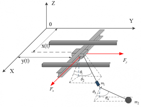
As illustrated in Figure 1, the 6-DOF overhead crane model is presented.
Movement of the trolley occurs along the $x$-axis and $y$-axis. under the corresponding forces $F_x$ and $F_y$, and is subject to air resistance with coefficients $d_x$ and $d_y$, as well as friction forces $F_{r x}$ and $F_{r y}$, respectively; $x$ and $y$ are position of the trolley along the x -axis and y -axis, respectively. During payload transportation, the swing angle hook with angles $\theta_1$ and $\theta_2$ in the horizontal ($x$) and vertical ($y$) directions, respectively, and is affected by air resistance with coefficients $d_1$ and $d_2$. The payload oscillations along the $x$-axis and $y$ axis are denoted by $\theta_3$ and $\theta_4$, subject to air resistance with coefficients $d_3$ and $d_4$. The friction forces $F_{r x}$ and $F_{r y}$ are determined according to the study [24] as follows:
$\left\{\begin{array}{l}F_{r x}=f_{r x} \tanh \left(\dot{x} / \varepsilon_x\right)+k_{r x}|\dot{x}| \dot{x} \\ F_{r y}=f_{r y} \tanh \left(\dot{y} / \varepsilon_y\right)+k_{r y}|\dot{y}| \dot{y}\end{array}\right.$ (1)
where, $f_{r x}, f_{r y}, \varepsilon_x$, and $\varepsilon_y$ denote friction at rest coefficients, while $k_{r x}$ and $k_{r y}$ represent the viscous friction coefficients.
Figure 1. Three-dimensional crane model with a double pendulum
The Euler–Lagrange equations are employed to describe the dynamics of the crane system featuring a 3D double pendulum [12].
$\mathbf{M}(\mathbf{q}) \ddot{\mathbf{q}}+\mathbf{C}(\mathbf{q}, \dot{\mathbf{q}}) \dot{\mathbf{q}}+\mathbf{G}(\mathbf{q})+\mathbf{D}=\mathbf{F}-\mathbf{U}_f$ (2)
where, $\mathbf{q}=\left[x, y, \theta_1, \theta_2, \theta_3, \theta_4\right]^T$ is the state vector of the system; $\mathbf{M}(\mathbf{q}) \in R^{6 \times 6}$ is the inertia matrix; $\mathbf{C}(\mathbf{q}, \dot{\mathbf{q}}) \in R^{6 \times 6}$ denotes the Coriolis-centrifugal matrix; $\mathbf{G}(\mathbf{q}) \in R^{6 \times 1}$ is the gravity vector; $\mathbf{D} \in R^{6 \times 1}$ represents external disturbances; and $\mathbf{F} \in R^{6 \times 1}$ is the control input vector; $\mathbf{U}_f \in R^{6 \times 1}$ denotes the friction/resistance forces of the system. The specific matrices and vectors are given as follows:
$\mathbf{M}(\mathbf{q})=\left[\begin{array}{llllll}M_{11} & M_{12} & M_{13} & M_{14} & M_{15} & M_{16} \\ M_{21} & M_{22} & M_{23} & M_{24} & M_{25} & M_{26} \\ M_{31} & M_{32} & M_{33} & M_{34} & M_{35} & M_{36} \\ M_{41} & M_{42} & M_{43} & M_{44} & M_{45} & M_{46} \\ M_{51} & M_{52} & M_{53} & M_{54} & M_{55} & M_{56} \\ M_{61} & M_{62} & M_{63} & M_{64} & M_{65} & M_{66}\end{array}\right] ;$
$\mathbf{C}(\mathbf{q}, \dot{\mathbf{q}})=\left[\begin{array}{llllll}C_{11} & C_{12} & C_{13} & C_{14} & C_{15} & C_{16} \\ C_{21} & C_{22} & C_{23} & C_{24} & C_{25} & C_{26} \\ C_{31} & C_{32} & C_{33} & C_{34} & C_{35} & C_{36} \\ C_{41} & C_{42} & C_{43} & C_{44} & C_{45} & C_{46} \\ C_{51} & C_{52} & C_{53} & C_{54} & C_{55} & C_{56} \\ C_{61} & C_{62} & C_{63} & C_{64} & C_{65} & C_{66}\end{array}\right] ;$
$\mathbf{G}=\left[\begin{array}{llllll}0 & 0 & G_{33} & G_{44} & G_{55} & G_{66}\end{array}\right]^T ;$
$\mathbf{F}=\left[\begin{array}{llllll}F_x & F_y & 0 & 0 & 0 & 0\end{array}\right]^T ;$
$\mathbf{U}_f=\left[\begin{array}{llllll}F_{r x}+d_x \dot{x} & F_{r y}+d_y \dot{y} & d_1 \dot{\theta}_1 & d_2 \dot{\theta}_2 & d_3 \dot{\theta}_3 & d_4 \dot{\theta}_4\end{array}\right]^T$.
The detailed components of the matrices and vectors can be found in the study [17].
$M_{11}=M_1+m_1+m_2 ; M_{12}=M_{21}=0 ;$
$M_{13}=M_{31}=\left(m_1+m_2\right) l_1 C_1 C_2 ;$
$M_{14}=M_{41}=-\left(m_1+m_2\right) l_1 S_1 S_2 ;$
$M_{15}=M_{51}=m_2 l_2 C_3 C_4 ; M_{16}=M_{61}=-m_2 l_2 S_3 S_4 ;$
$M_{22}=M_2+m_1+m_2 ; M_{23}=M_{32}=0 ;$
$M_{24}=M_{42}=\left(m_1+m_2\right) l_1 C_2 ; M_{25}=M_{52}=0 ;$
$M_{26}=M_{62}=m_2 l_2 C_4 ; M_{33}=\left(m_1+m_2\right) l_1^2 C_2^2 ;$
$M_{34}=M_{43}=0 ;$
$M_{35}=M_{53}=m_2 l_1 l_2\left(C_1 C_2 C_3 C_4+S_1 C_2 S_3 C_4\right) ;$
$M_{36}=M_{63}=m_2 l_1 l_2\left(S_1 C_2 C_3 S_4-C_1 C_2 S_3 S_4\right) ;$
$M_{44}=\left(m_1+m_2\right) l_1^2 ;$
$M_{45}=M_{54}=m_2 l_1 l_2\left(C_1 S_2 S_3 C_4-S_1 S_2 C_3 C_4\right)$
$M_{46}=M_{64}=m_2 l_1 l_2\left(C_2 C_4+C_1 S_2 C_3 S_4+S_1 S_2 S_3 S_4\right) ;$
$M_{55}=m_2 l_2^2 C_4^2 ; M_{56}=M_{65}=0 ; M_{66}=m_2 l_2^2$
$C_{11}=F_{r x} ; \quad C_{12}=0 ;$
$C_{13}=-\left(m_1+m_2\right) l_1\left(S_1 C_2 \dot{\theta}_1+C_1 S_2 \dot{\theta}_2\right) ;$
$C_{14}=-\left(m_1+m_2\right) l_1\left(C_1 S_2 \dot{\theta_1}+S_1 C_2 \dot{\theta_2}\right) ;$
$C_{15}=-m_2 l_2\left(S_3 C_4 \dot{\theta}_3+C_3 S_4 \dot{\theta}_4\right) ;$
$C_{16}=-m_2 l_2\left(C_3 S_4 \dot{\theta}_3+S_3 C_4 \dot{\theta}_4\right) ; C_{21}=0 ; C_{22}=F_{r y} ;$
$C_{23}=0 ; C_{24}=-\left(m_1+m_2\right) l_1 S_2 \dot{\theta}_2 ; C_{25}=0 ;$
$C_{26}=-m_2 l_2 S_4 \dot{\theta}_4 ; \quad C_{31}=0 ; C_{32}=0 ;$
$C_{26}=-m_2 l_2 S_4 \dot{\theta}_4 ; \quad C_{31}=0 ; C_{32}=0 ;$
$C_{33}=-\left(m_1+m_2\right) l_1^2 S_2 C_2 \dot{\theta}_2 ;$
$C_{34}=-\left(m_1+m_2\right) l_1^2 S_2 C_2 \dot{\theta_1} ;$
$C_{35}=m_2 l_1 l_2 S_{1-3}\left(C_2 C_4 \dot{\theta}_3+S_2 S_4 \dot{\theta}_4\right) ;$
$C_{36}=-m_2 l_1 l_2 C_2\left(C_1 C_3 S_4 \dot{\theta}_3+S_1 S_3 S_4 \dot{\theta}_3+C_1 S_3 C_4 \dot{\theta}_4-S_1 C_3 C_4 \dot{\theta}_4\right) ;$
$C_{41}=0 ; \quad C_{42}=0 ; \quad C_{43}=\left(m_1+m_2\right) l_1^2 S_2 C_2 \dot{\theta}_1 ; \quad C_{44}=0 ;$
$C_{45}=m_2 l_1 l_2 S_2\left(C_1 C_3 C_4 \dot{\theta}_3+S_1 S_3 C_4 \dot{\theta}_3-C_1 S_3 S_4 \dot{\theta}_4+S_1 C_3 S_4 \dot{\theta}_4\right)$
$\begin{gathered}C_{46}=m_2 l_1 l_2\left(C_1 S_2 C_3 C_4 \dot{\theta}_4+S_1 S_2 S_3 C_4 \dot{\theta}_4-C_2 S_4 \dot{\theta}_4\right. \\ \left.-C_1 S_2 S_3 S_4 \dot{\theta}_3+S_1 S_2 C_3 S_4 \dot{\theta}_3\right) ; \\ C_{51}=0 ; C_{52}=0 ; \\ C_{53}=-m_2 l_1 l_2 C_4\left(S_1 C_2 C_3 \dot{\theta}_1-C_1 C_2 S_3 \dot{\theta}_1+C_1 S_2 C_3 \dot{\theta}_2+S_1 S_2 S_3 \dot{\theta}_2\right) ; \\ C_{54}=-m_2 l_1 l_2 C_4\left(C_1 S_2 C_3 \dot{\theta}_1+S_1 S_2 S_3 \dot{\theta}_1-C_1 C_2 S_3 \dot{\theta}_2+S_1 C_2 C_3 \dot{\theta}_2\right) ;\end{gathered}$
$\begin{gathered}C_{55}=-m_2 l_2^2 S_4 C_4 \dot{\theta}_4 ; \quad C_{56}=-m_2 l_2^2 S_4 C_4 \dot{\theta}_3 ; \\ C_{61}=0 ; C_{62}=0 ; \\ C_{63}=m_2 l_1 l_2 S_4\left(C_1 C_2 C_3 \dot{\theta}_1+S_1 C_2 S_3 \dot{\theta}_1+C_1 C_2 S_3 \dot{\theta}_2-S_1 S_2 C_3 \dot{\theta}_2\right) ; \\ C_{64}=m_2 l_1 l_2\left(C_1 C_2 C_3 S_4 \dot{\theta}_2+S_1 C_2 S_3 S_4 \dot{\theta}_2-S_2 C_4 \dot{\theta}_2\right. \\ \left.+C_1 S_2 S_3 S_4 \dot{\theta}_1-S_1 S_2 C_3 S_4 \dot{\theta}_1\right) ; \\ C_{65}=m_2 l_2^2 S_4 C_4 \dot{\theta}_3 ; C_{66}=0 ; \\ G_{33}=\left(m_1+m_2\right) g l_1 S_1 C_2 ; G_{44}=\left(m_1+m_2\right) g l_1 C_1 S_2 ; \\ G_{55}=m_2 g l_2 S_3 C_4 ; G_{66}=m_2 g l_2 C_3 S_4 ; \\ \text { with } C_i=\cos \theta_i ; S_i=\sin \theta_i ;(i=1 \div 4)\end{gathered}$
where, $M_1$ and $M_2$ are trolley mass along x -axis and y -axis, respectively; $m_1$ is hook mass; $m_2$ denotes payload mass; $l_1$ and $l_2$ denote hook length vaf cable length, respectively.
The objective of controlling the 3D double-pendulum overhead crane system (3DDOC) must achieve two simultaneous goals: (i) the actuated state variables $x(t)$ and $y(t)$ are controlled to follow a trajectory to the desired position $\left(x_d, y_d\right), x(t) \rightarrow x_d, y(t) \rightarrow y_d$; and (ii) the unactuated state variables $\theta_i(i=1 \div 4)$ are suppressed to zero, $\theta_i \rightarrow 0$. To facilitate the controller design for the 3DDOC system, the system is divided into two subsystems: the actuated subsystem and the unactuated subsystem, corresponding to the state variables $\mathbf{q}_a=[x, y]^T$ and $\mathbf{q}_u= \left[\theta_1, \theta_2, \theta_3, \theta_4\right]^T$, respectively. The system dynamics (2) can then be rewritten as follows:
$\begin{aligned} & \mathbf{M}_{a a}(\mathbf{q}) \ddot{\mathbf{q}}_a+\mathbf{M}_{a u}(\mathbf{q}) \ddot{\mathbf{q}}_u+\mathbf{C}_{a a}(\mathbf{q}, \dot{\mathbf{q}}) \dot{\mathbf{q}}_a+\mathbf{C}_{a u}(\mathbf{q}, \dot{\mathbf{q}}) \dot{\mathbf{q}}_u +\mathbf{G}_{a a}(\mathbf{q})+\mathbf{D}_{a a}=\mathbf{F}_a-\mathbf{U}_{f a}\end{aligned}$ (3)
$\begin{aligned} & \mathbf{M}_{u a}(\mathbf{q}) \ddot{\mathbf{q}}_a+\mathbf{M}_{u u}(\mathbf{q}) \ddot{\mathbf{q}}_u+\mathbf{C}_{u a}(\mathbf{q}, \dot{\mathbf{q}}) \dot{\mathbf{q}}_a+\mathbf{C}_{u u}(\mathbf{q}, \dot{\mathbf{q}}) \dot{\mathbf{q}}_u +\mathbf{G}_{u u}(\mathbf{q})+\mathbf{D}_{u u}=-\mathbf{U}_{f u}\end{aligned}$ (4)
where:
$\begin{aligned} & \mathbf{M}_{a a}(\mathbf{q})=\left[\begin{array}{ll}M_{11} & M_{12} \\ M_{21} & M_{22}\end{array}\right] ; \mathbf{M}_{a u}=\left[\begin{array}{llll}M_{13} & M_{14} & M_{15} & M_{16} \\ M_{23} & M_{24} & M_{25} & M_{26}\end{array}\right] \\ & \mathbf{M}_{u a}(\mathbf{q})=\left[\begin{array}{ll}M_{31} & M_{32} \\ M_{41} & M_{42} \\ M_{51} & M_{52} \\ M_{61} & M_{62}\end{array}\right] ; \mathbf{M}_{u u}=\left[\begin{array}{llll}M_{33} & M_{34} & M_{35} & M_{36} \\ M_{43} & M_{44} & M_{45} & M_{46} \\ M_{53} & M_{54} & M_{55} & M_{56} \\ M_{63} & M_{64} & M_{65} & M_{66}\end{array}\right] ;\end{aligned}$
$\mathbf{C}_{a a}(\mathbf{q}, \dot{\mathbf{q}})=\left[\begin{array}{ll}C_{11} & C_{12} \\ C_{21} & C_{22}\end{array}\right] ;$
$\mathbf{C}_{a u}(\mathbf{q}, \dot{\mathbf{q}})=\left[\begin{array}{llll}C_{13} & C_{14} & C_{15} & C_{16} \\ C_{23} & C_{24} & C_{25} & C_{26}\end{array}\right]$
$\mathbf{C}_{u a}(\mathbf{q}, \dot{\mathbf{q}})=\left[\begin{array}{ll}C_{31} & C_{32} \\ C_{41} & C_{42} \\ C_{51} & C_{52} \\ C_{61} & C_{62}\end{array}\right]$;
$\mathbf{C}_{u u}(\mathbf{q}, \dot{\mathbf{q}})=\left[\begin{array}{llll}C_{33} & C_{34} & C_{35} & C_{36} \\ C_{43} & C_{44} & C_{45} & C_{46} \\ C_{53} & C_{54} & C_{55} & C_{56} \\ C_{63} & C_{64} & C_{65} & C_{66}\end{array}\right]$
$\mathbf{G}_{a a}=[0,0]^T ; \mathbf{G}_{u u}=\left[G_{33}, G_{44}, G_{55}, G_{66}\right]^T ; \mathbf{D}_{a a} \in R^{2,1} ;$
$\mathbf{D}_{u u} \in R^{4,1} ; \mathbf{F}_a=\left[F_x, F_y\right]^T ; \mathbf{U}_{f a}=\left[F_{r x}+d_x \dot{x}, F_{r y}+d_y \dot{y}\right]^T ;$
$\mathbf{U}_{f l}=\left[\begin{array}{llll}d_1 \dot{\theta}_1 & d_2 \dot{\theta}_2 & d_3 \dot{\theta}_3 & d_4 \dot{\theta}_4\end{array}\right]^T$
From Eq. (4), it follows that $\ddot{\mathbf{q}}_u=\mathbf{h}_u(\mathbf{q}, \dot{\mathbf{q}})$, which is then substituted into Eq. (3). The system dynamics can be rewritten as a fully actuated system as follows:
$\mathbf{M}_a(\mathbf{q}) \ddot{\mathbf{q}}_a+\mathbf{h}_a(\mathbf{q}, \dot{\mathbf{q}})=\mathbf{F}_a$ (5)
$\begin{aligned} & \text { with } \mathbf{M}_a=\mathbf{M}_{a a}(\mathbf{q})-\mathbf{M}_{a u}(\mathbf{q}) \mathbf{M}_{u u}^{-1}(\mathbf{q}) \mathbf{M}_{u a}(\mathbf{q}) ; \mathbf{h}_a(\mathbf{q}, \dot{\mathbf{q}})=\left(\mathbf{C}_{a a}(\mathbf{q}, \dot{\mathbf{q}})-\mathbf{M}_{a u}(\mathbf{q}) \mathbf{M}_{u u}^{-1}(\mathbf{q}) \mathbf{C}_{u a}(\mathbf{q}, \dot{\mathbf{q}})\right) \dot{\mathbf{q}}_a \\ & +\left(\mathbf{C}_{a u}(\mathbf{q}, \dot{\mathbf{q}})-\mathbf{M}_{a u}(\mathbf{q}) \mathbf{M}_{u u}^{-1}(\mathbf{q}) \mathbf{C}_{u u}(\mathbf{q}, \dot{\mathbf{q}})\right) \dot{\mathbf{q}}_u+\mathbf{G}_{a a}+\mathbf{D}_{a a}+\mathbf{U}_{f a} -\mathbf{M}_{a u}(\mathbf{q}) \mathbf{M}_{u u}^{-1}(\mathbf{q})\left(\mathbf{G}_{u u}+\mathbf{D}_{u u}+\mathbf{U}_{f u}\right) .\end{aligned}$.
The nominal mass matrix of $\mathbf{M}_a(\mathbf{q})$ is defined as $\mathbf{M}_{\text {const}}$. Eq. (5) can be rewritten as follows:
$\mathbf{M}_{\text {const }} \ddot{\mathbf{q}}_a+\mathbf{f}_a(\mathbf{q}, \dot{\mathbf{q}}, \ddot{\mathbf{q}})=\mathbf{F}_a$ (6)
where: $\mathbf{M}_{\text {const }}=\operatorname{diag}\left(M_{\text {const } 1}, M_{\text {const } 2}\right)$, with $M_{\text {const } 1}$ and $M_{\text {const } 2}$ are positive coefficients $\mathbf{f}_a(\mathbf{q}, \dot{\mathbf{q}}, \ddot{\mathbf{q}})=\left(\mathbf{M}_a-\right. \left.\mathbf{M}_{\text {const }}\right) \ddot{\mathbf{q}}_a+\mathbf{h}_a$.
In Eq. (6), the uncertainties and external disturbances of the 3DDOC system are contained in the vector $\mathbf{f}_a(\mathbf{q}, \dot{\mathbf{q}}, \ddot{\mathbf{q}})$.
Based on the relationship between the actuated and unactuated state variables, the signal error is defined as follows:
$\mathbf{e}=\mathbf{q}_a-\mathbf{q}_r-\mathbf{q}_{l u}$ (7)
with $\mathbf{q}_r=\left[x_r, y_r\right]^T$, the reference trajectory of the trolley when moving along the axis $x$, axis $y ; \mathbf{e}_a=\mathbf{q}_a-\mathbf{q}_r$: tracking error of position control; $\mathbf{q}_{l u}=\left[l_1 \theta_1+l_2 \theta_3 \quad l_1 \theta_2+l_2 \theta_4\right]$.
The sliding surface is designed with the following structure:
$\mathbf{s}=\dot{\mathbf{e}}+\Gamma \mathbf{e}$ (8)
with $\boldsymbol{\Gamma}=\operatorname{diag}\left(\Gamma_1, \Gamma_2\right)$ is the matrix of positive coefficients and the sliding surface matrix. The derivative of the sliding surface (8) with respect to time is expressed as:
$\begin{aligned} \dot{\mathbf{s}} & =\ddot{\mathbf{e}}+\boldsymbol{\Gamma} \dot{\mathbf{e}} \\ & =\ddot{\mathbf{q}}_a-\left(\ddot{\mathbf{q}}_r+\ddot{\mathbf{q}}_{l u}-\boldsymbol{\Gamma} \dot{\mathbf{e}}\right) \\ & =\ddot{\mathbf{q}}_a-\ddot{\mathbf{q}}_{a c}\end{aligned}$ (9)
where: $\ddot{\mathbf{q}}_{a c}=\ddot{\mathbf{q}}_r+\ddot{\mathbf{q}}_{l u}-\boldsymbol{\Gamma} \dot{\boldsymbol{e}}$, with $\ddot{\mathbf{q}}_r=\left[\ddot{x}_r, \ddot{y}_r\right]^T ; \ddot{\mathbf{q}}_{l u}=\begin{aligned}& {\left[l_1 \ddot{\theta_1}+l_2 \ddot{\theta_3} \quad l_1 \ddot{\theta_2}+l_2 \ddot{\theta}_4\right]^T ; \dot{\mathbf{e}}=\dot{\mathbf{q}}_a-\dot{\mathbf{q}}_r-\dot{\mathbf{q}}_{l u} ; \dot{\mathbf{q}}_a=[\dot{x},} \dot{y}]^T ; \dot{\mathbf{q}}_r=\left[\dot{x}_r, \dot{y}_r\right]^T ; \dot{\mathbf{q}}_{l u}=\left[l_1 \dot{\theta_1}+l_2 \dot{\theta_3} \quad l_1 \dot{\theta_2}+l_2 \dot{\theta}_4\right]^T\end{aligned}$.
An adaptive sliding mode controller leveraging time-delay estimation (ASMC-TDE) is proposed as follows:
$\mathbf{F}_a=\hat{\mathbf{f}}_a+\mathbf{M}_{\text {const }}\left(\ddot{\mathbf{q}}_{a c}-\Lambda \operatorname{sign}(\mathbf{s})-\mathbf{K s}\right)$ (10)
$\hat{\mathbf{f}}_a$ is the estimate of $\mathbf{f}_a$. Then, the estimation error is defined as:
$\boldsymbol{\sigma}=\hat{\mathbf{f}}_a-\mathbf{f}_a$ (11)
Meanwhile, $\boldsymbol{\Lambda}=\operatorname{diag}\left(\Lambda_1, \Lambda_2\right)$ is switching gain matrix and matrice $\mathbf{K}=\operatorname{diag}\left(K_1, K_2\right)$ is linear gain matrix, where $\Lambda_1$ and $\Lambda_2$ are chosen such that $\Lambda_{\text {min }}=\min \left(\Lambda_1, \Lambda_2\right)_{\text {}}$, with $\xi= \left\|\mathbf{M}_{\text {const }}^{-1} \boldsymbol{\sigma}\right\|$.
Using the time-delay estimation technique [25] the estimate $\hat{\mathbf{f}}_a$ is structured as follows:
$\hat{\mathbf{f}}_a=\mathbf{f}_{a(t-T)}=\mathbf{F}_{a(t-T)}-\mathbf{M}_{\mathrm{const}} \ddot{\mathbf{q}}_{a(t-T)}$ (12)
where, T is a very small time delay, selected to be the same as the sampling time (TDE).
The parameters in the proposed ASMC-TDE controller are systematically selected to ensure Lyapunov stability and optimize tracking performance, while effectively mitigating chattering:
$\boldsymbol{\Gamma}$ is chosen such that the eigenvalues of $\boldsymbol{\Gamma}$ establish the desired exponential convergence rate of the error to zero.
$\mathbf{M}_{\text {const}}$ must be chosen as a constant, positive definite matrix that is the best approximation of the actual mass matrix $\mathbf{M}_a(\boldsymbol{q})$ to minimize the residual uncertainty.
T is set equal to the smallest possible sampling period of the discrete-time control system to minimize the TDE estimation error.
$\boldsymbol{\Lambda}$ is a positive diagonal matrix determined by the upper bound of the residual uncertainty.
$\mathbf{K}$ is selected through simulation tuning to balance a fast transient response with the need to avoid actuator saturation.
Theorem 3.1. The sliding surface designed in Eq. (8), the proposed controller in Eq. (10), and the uncertainties and disturbances estimated in Eq. (12) are employed for the 3DDOC system. The signal error e will converge to zero. Simultaneously, the actuated state variables $x$ and $y$ converge to the desired positions $x_d$ and $y_d$ $\left(x \rightarrow x_d, y \rightarrow y_d\right)$, and the swing angles of the hook and payload will converge to zero ($\theta_i \rightarrow 0$).
Proof: The following is the chosen candidate Lyapunov function:
$V=\frac{1}{2} \mathbf{s}^T \mathbf{s}$ (13)
By differentiating the Lyapunov function (13) with respect to time and subsequently substituting (9) and (10) into it, we obtain:
$\begin{array}{cc}\dot{V}= & \mathbf{s}^T\left(\mathbf{M}_{\text {const }}^{-1}\left(\hat{\mathbf{f}}_a-\mathbf{f}_a\right)-\boldsymbol{\Lambda} \operatorname{sign}(\mathbf{s})-\mathbf{K} \mathbf{s}\right) \\ = & \mathbf{s}^T\left(\mathbf{M}_{\text {const }}^{-1} \sigma-\boldsymbol{\Lambda} \operatorname{sign}(\mathbf{s})-\mathbf{K} \mathbf{s}\right) \\ \leqslant & -\left(\Lambda_{\text {min }}-\xi\right)| | \mathbf{s}| |-\mathbf{s}^T \mathbf{K} \mathbf{s} \leqslant 0\end{array}$ (14)
By applying the Lyapunov stability principle, it is ensured that the system is stable and the sliding surface $\mathbf{s}$ reaches zero, $\mathbf{s} \rightarrow 0$ as $t \rightarrow \infty$. This implies that $\dot{\mathbf{e}}+\boldsymbol{\Gamma} \rightarrow 0$. For this firstorder differential equation, the solution is expressed as $e_i= e^{-\Gamma_i t} \rightarrow 0$.
When the system reaches stability, the following equation holds:
$\begin{aligned} & x=l_1 \theta_1+l_2 \theta_3+x_d ; \quad \dot{x}=l_1 \dot{\theta}_1+l_2 \dot{\theta}_3 \\ & y=l_1 \theta_2+l_2 \theta_4+y_d ; \quad \dot{y}=l_1 \dot{\theta}_2+l_2 \dot{\theta}_4\end{aligned}$ (15)
where: $\dot{\mathbf{q}}_a=[\dot{x}, \dot{y}]^T=\mathbf{K}_u \dot{\mathbf{q}}_u$, with $\mathbf{K}_u=\left[\begin{array}{cccc}l_1 & 0 & l_2 & 0 \\ 0 & l_1 & 0 & l_2\end{array}\right]$; $\ddot{\mathbf{q}}_a=\mathbf{K}_u \ddot{\mathbf{q}}_u$.
Since the hook and payload swing angles are typically small during the trolley motion, it is reasonable to approximate $\cos \theta_i \approx 1$ and $\sin \theta_i \approx \theta_i$. Consequently:
$\mathbf{M}_{u a} \approx\left[\begin{array}{cc}\left(m_1+m_2\right) l_1 & 0 \\ 0 & \left(m_1+m_2\right) l_1 \\ m_2 l_2 & 0 \\ 0 & m_2 l_2\end{array}\right] ;$
$\mathbf{M}_{u u} \approx\left[\begin{array}{cccc}\left(m_1+m_2\right) l_1^2 & 0 & m_2 l_1 l_2 & 0 \\ 0 & \left(m_1+m_2\right) l_1^2 & 0 & m_2 l_1 l_2 \\ m_2 l_1 l_2 & 0 & m_2 l_2^2 & 0 \\ 0 & m_2 l_1 l_2 & 0 & m_2 l_2^2\end{array}\right] ;$
$\begin{gathered}\mathbf{G}_{u u} \approx\left[\left(m_1+m_2\right) g l_1 \theta_1,\left(m_1+m_2\right) g l_1 \theta_2, m_2 g l_2 \theta_3, m_2 g l_2 \theta_4\right]^T \\ =\mathbf{K}_G \mathbf{q}_u\end{gathered}$
with $\mathbf{K}_G=\operatorname{diag}\left(\left(m_1+m_2\right) g l_1,\left(m_1+m_2\right) g l_1, m_2 g l_2, m_2 g l_2\right)$.
$\mathbf{C}_{u a}(\mathbf{q}, \dot{\mathbf{q}}) \approx\left[\begin{array}{ll}0 & 0 \\ 0 & 0 \\ 0 & 0 \\ 0 & 0\end{array}\right] ; \mathbf{C}_{u u}(\mathbf{q}, \dot{\mathbf{q}}) \approx\left[\begin{array}{lll}0 & 0 & 0 \\ 0 & 0 & 0 \\ 0 & 0 & 0 \\ 0 & 0 & 0\end{array}\right]$
This is because most components of the $\mathbf{C}_{u a}(\mathbf{q}, \dot{\mathbf{q}})$ and $\mathbf{C}_{u u}(\mathbf{q}, \dot{\mathbf{q}})$ are approximately zero, as they contain products of angles $\left(\theta_i\right)$ with angular velocities $\left(\dot{\theta_i}\right)$, which are treated as higher-order terms.
From the above approximation and Eq. (4), we obtain:
$\begin{aligned} & \mathbf{M}_{u a} \mathbf{K}_u \ddot{\mathbf{q}}_u+\mathbf{M}_{u u} \ddot{\mathbf{q}}_u+\mathbf{C}_{u a} \mathbf{K}_u \dot{\mathbf{q}}_u+\mathbf{C}_{u u} \dot{\mathbf{q}}_u +\mathbf{K}_G \mathbf{q}_u+\mathbf{d} \dot{\mathbf{q}}_u=0\end{aligned}$ (16)
with $\mathbf{d}=\operatorname{diag}\left(d_1, d_2, d_3, d_4\right)$.
The underactuated dynamic Eq. (16) can be rewritten as follows:
$\ddot{\mathbf{q}}_u=-\mathbf{H}_a \mathbf{K}_G \mathbf{q}_u-\mathbf{H}_a\left(\mathbf{C}_{u a} \mathbf{K}_u+\mathbf{C}_{u u}+\mathbf{d}\right) \dot{\mathbf{q}}_u$ (17)
where, $\mathbf{H}_a=\left(\mathbf{M}_{u a} \mathbf{K}_u+\mathbf{M}_{u u}\right)^{-1}$.
The state vector $\mathbf{z} \in R^{8 \times 1}$ representing the swing angles and angular velocities of the hook and payload is defined as follows:
$\mathbf{z}=\left[\mathbf{q}_u, \dot{\mathbf{q}}_u\right]^T$ (18)
Based on Eq. (18), Eq. (17) can be rewritten as follows:
$\dot{\mathbf{z}}=\mathbf{B} \mathbf{z}$ (19)
in which the state matrix B is described as follows:
$\begin{aligned} \mathbf{B}= & {\left[\begin{array}{cc}\mathbf{0}_{4 \times 4} & \mathbf{I}_{4 \times 4} \\ \mathbf{B}_1 & \mathbf{B}_2\end{array}\right], \text { with } \mathbf{B}_1=-\mathbf{H}_a \mathbf{K}_G ; } \\ & \mathbf{B}_2=-\mathbf{H}_a\left(\mathbf{C}_{u a} \mathbf{K}_u+\mathbf{C}_{u u}+\mathbf{d}\right)\end{aligned}$
The characteristic equation of B is given as follows:
$\left|\lambda \mathbf{I}_{4 \times 4}-\mathbf{B}\right|=0$ (20)
Considering the parameters of the 3DDOC system, the eigenvalues of Eq. (20) all have real parts located on the left half of the imaginary axis, hence the system Eq. (17) is asymptotically stable. This means that:
$\lim _{t \rightarrow \infty} \mathbf{z}=0$ (21)
Substituting Eq. (21) into Eq. (15), we obtain:
$\lim _{t \rightarrow \infty}\left[\begin{array}{llll}x & y & \dot{x} & \dot{y}\end{array}\right]^T=\left[\begin{array}{llll}x_d & y_d & 0 & 0\end{array}\right]^T$ (22)
Figure 2. The designed control scheme
Hence, the proof of Theorem 3.1 is complete.
The operation of the 3DDOC system under ASMC-TDE control is illustrated in Figure 2, which presents the closed-loop block diagram.
This section evaluates the performance of the proposed controller through MATLAB/SIMULINK simulations. In order to evaluate the effectiveness and robustness of the proposed adaptive controller Eq. (10), two the simulations will be carried out in comparison with the sliding mode controller designed to restrict the swing angles of both the hook and the payload. Two simulation scenarios will be performed:
The following are the parameters of the system:
$\begin{gathered}M_1=15 \mathrm{~kg} ; M_2=35 \mathrm{~kg} ; m_1=5 \mathrm{~kg} ; m_2=5 \mathrm{~kg} ; l_1=1 \mathrm{~m} ; \\ l_2=0.2 \mathrm{~m} ; g=9.8 \mathrm{~m} / \mathrm{s}^2 ;\end{gathered}$
The payload starts at coordinates $\left[x_0, y_0\right]=[0,0](m)$ and needs to reach the desired position $\left\lceil x_d, y_d\right\rceil=\lceil 3,3\rceil(m)$. Both its initial and final velocities and accelerations are set to zero. The travel time for the payload to reach the desired position is $T_x=30 \mathrm{~s}$ for movement along the $x$-axis and $T_y=$ 20 s for the $y$-axis. The trajectory of the payload is detailed below:
$x_r$$=\left\{\begin{array}{cl}6 x_d\left(\frac{t}{T_x}\right)^5-15 x_d\left(\frac{t}{T_x}\right)^4+10 x_d\left(\frac{t}{T_x}\right)^3 & , t \leqslant T_x \\ x_d & , t>T_x\end{array}\right.$ (23)
$y_r=\left\{\begin{array}{cl}6 y_d\left(\frac{t}{T_y}\right)^5-15 y_d\left(\frac{t}{t_y}\right)^4+10 y_d\left(\frac{t}{T_y}\right)^3 & , t \leqslant T_y \\ y_d & , t>T_y\end{array}\right.$ (24)
All initial and simulation conditions are summarized in Table 1.
The sliding mode controller designed to constrain the swing angles of both the hook and the payload (Sliding Mode Controller with Swing Angle Constraint) (SMC-SAC) is given in Eq. (25).
Table 1. Simulation conditions
|
Parameter Category |
Symbol |
Value |
Unit |
|
I. Initial Conditions |
|
|
|
|
Trolley position (x) |
x(0) |
0 |
m |
|
Trolley position (y) |
y(0) |
0 |
m |
|
Hook swing angle (x-z plane) |
$\theta_1(0)$ |
0.052 |
rad |
|
Hook swing angle (y-z plane) |
$\theta_2(0)$ |
0.052 |
rad |
|
Payload swing angle (x-z plane) |
$\theta_3(0)$ |
0.052 |
rad |
|
Payload swing angle (y-z plane) |
$\theta_4(0)$ |
0.052 |
rad |
|
All initial and final velocities |
$\dot{\mathbf{q}}(0), \dot{\mathbf{q}}_f$ |
0 |
m/s or rad/s |
|
All initial and final accelerations |
$\ddot{\mathbf{q}}(0), \ddot{\mathbf{q}}_f$ |
0 |
m/s2 or rad/s2 |
|
II. Trajectory/reference |
|
|
|
|
x-reference trajectory |
xd(t) |
Fifth-order polynomial |
m |
|
Reference trajectory time for the x-axis |
$T_x$ |
30 |
s |
|
y-reference trajectory |
yd(t) |
Fifth-order polynomial |
m |
|
Reference trajectory time for the y-axis |
$T_y$ |
20 |
s |
|
Total simulation time |
tsim |
50 |
s |
|
III. External Disturbances |
|
|
|
|
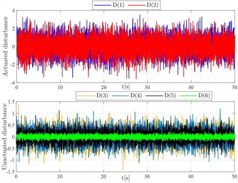
Disturbance applied to x |
D(1) |
$8 \sin \left(105 \pi \mathrm{t}+\frac{\pi}{6}\right)$ |
N |
|
Disturbance applied to y |
D(2) |
8sin$\left(85 \pi \mathrm{t}+\frac{2 \pi}{3}\right)$ |
N |
|
Disturbance applied to hook |
D(3), D(4) |
0.4sin$(85 \pi \mathrm{t})$ |
N |
|
Disturbance applied to payload |
D(5), D(6) |
0.4sin$(100 \pi \mathrm{t})$ |
N |
|
IV. Control Parameters |
|
|
|
|
Sampling Time (TDE) |
T |
0.002 |
s |
|
Sliding surface matrix |
$\Gamma$ |
diag(12,15) |
|
|
Nominal mass matrix |
$\mathbf{M}_{\text {const }}$ |
diag(0.7,0.7) |
|
|
Switching gain matrix |
$\Lambda$ |
diag(1.5,2.5) |
|
|
Linear gain matrix |
K |
diag(5,10) |
|
$\mathbf{F}_{a s}=\mathbf{f}_a+\mathbf{M}_{\text {const }}\left(\ddot{\mathbf{q}}_{a c}-\boldsymbol{\Lambda}_s \operatorname{sign}(\mathbf{s})-\mathbf{K}_s \mathbf{s}\right)$ (25)
The parameters of the controller are chosen as follows: $\boldsymbol{\Lambda}_s=\operatorname{diag}(10,13), \mathbf{K}_s=\operatorname{diag}(5,10)$.
4.1 Scenario 1
In this section, simulations are performed under conditions where the system parameters remain constant, but the system experiences external disturbances given by:
$\begin{aligned} \mathbf{D}= & {\left[\begin{array}{lll}8 \sin (105 \pi t+\pi / 6) & 8 \sin (85 \pi t+2 \pi / 3) & 0.4 \sin (85 \pi t) \\ & 0.4 \sin (85 \pi t) & 0.4 \sin (100 \pi t) \\ & 0.4 \sin (100 \pi t)\end{array}\right]^T }\end{aligned}$
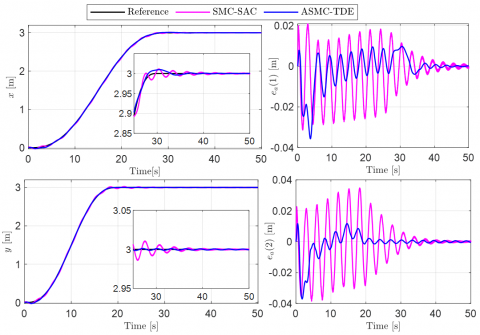
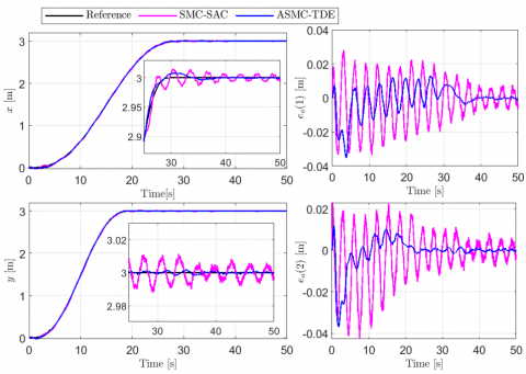
The outcomes of Scenario 1 are presented in Figures 3-6.
Figure 3. Position trajectory and the corresponding errors (Scenario 1)
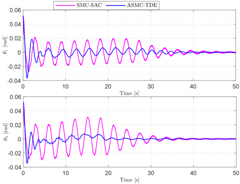
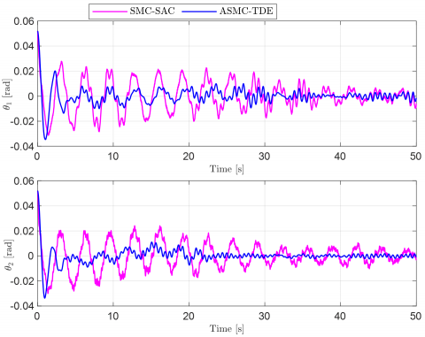
Figure 4. Swing angles of the hook (Scenario 1)
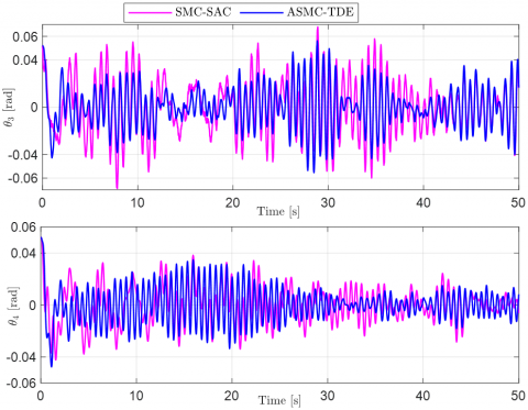
Figure 5. Swing angles of the payload (Scenario 1)
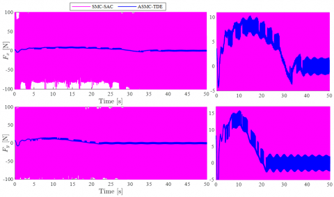
Figure 6. The force acting on the trolley (Scenario 1)
4.2 Scenario 2
The robustness and adaptive capability of the proposed controller are validated through system simulations under the following conditions: the payload mass is increased to 6kg, and the cable length l1 is increased by 1.2 times. In particular, the system is also subjected to a more severe and pronounced external disturbance compared to Scenario 1, specifically white noise, as illustrated in Figure 7. The results of the second scenario are presented in Figures 8-11. The performance indices of the state variables, which use ISE, ITSE, IAE, and ITAE as evaluation criteria, are also shown in Tables 2 and 3.
From the simulation results of the two scenarios, it can be seen that even under the influence of different types of disturbances: harmonic disturbance and random disturbance (white noise), with the system parameters changed, and with nonzero initial conditions for the swing angle of the hook and the payload, the system still operates stably. This is demonstrated through the position trajectories in Figure 3 and Figure 8, where the trajectories x(t) and y(t) track the reference trajectory with errors oscillating around zero with small amplitudes (< 4 cm) during the transient period, and then rapidly converge to zero as the payload reaches the desired position. However, ASMC-TDE significantly improves tracking accuracy and minimizes steady-state position error, demonstrating a much faster error convergence rate compared with the SMC-SAC controller. Given the initial condition that the hook swing angle at the beginning of the system motion is a nonzero value, the hook swing angle always remains within a very small bound, not exceeding its initial value, as shown in Figure 4 and Figure 9. Furthermore, ASMC-TDE significantly improves this performance. As for the payload oscillation, under all conditions, it also stays within a very small range, not exceeding 0.052 rad, as illustrated in Figure 5 and Figure 10. This superior ability to tightly constrain the oscillations confirms the outstanding stability and effectiveness of the proposed ASMC-TDE controller. Additionally, the force signals acting on the trolley, shown in Figure 6 and Figure 11, indicate that the control force varies, exhibiting oscillations with amplitudes that change over time. This demonstrates that the controller operates continuously to compensate for disturbances and uncertainties, and subsequently, the applied force gradually decreases and stabilizes as the payload reaches the desired position. Nevertheless, the ASMC-TDE is far superior to the SMC-SAC because it constrains the control force to a much smaller amplitude and rapidly decreases to zero in the steady state, whereas the SMC-SAC maintains the force at a large amplitude. Consequently, ASMC-TDE achieves superior control performance while offering significantly better energy efficiency and reduced mechanical wear compared to the SMC-SAC.
Figure 7. White noise acting on the system (Scenario 2)
Figure 8. Position trajectory and the corresponding errors (Scenario 2)
Figure 9. Swing angles of the hook (Scenario 2)
Figure 10. Swing angles of the payload (Scenario 2)
The performance indices in Table 2 and Table 3 show that the proposed controller outperforms the sliding mode controller designed to restrict the swing angles of both the hook and the payload, in terms of reducing error and improving the convergence speed of all output variables. For the trolley position, the ISE and ITSE indices are reduced by 60.4% and 79.5%, respectively, while the IAE and ITAE indices decrease by 53.7% and 68.1%, respectively. The reduction is even more significant for the hook swing angle, with decreases of 67.9% and 87.2%. The payload swing angle is also improved, but to a lesser extent, with reductions of 32.9% and 31% for ISE and ITSE, and 19.3% and 17.9% for IAE and ITAE, respectively. This indicates that reducing payload oscillations is more challenging due to inertia and coupling effects. Hence, the results demonstrate that the ASMC-TDE significantly outperforms the sliding mode controller designed to constrain the swing angles of the hook and payload in terms of improving tracking accuracy and minimizing error.
Figure 11. The force acting on the trolley (Scenario 2)
Table 2. Performance evaluation criteria: ISE and ITSE
|
Output Variable |
Control Strategy |
ISE |
ITSE |
|
Trolley position |
ASMC-TDE |
0.0077089 |
0.051702 |
|
ASMC |
0.019458 |
0.25214 |
|
|
Hook swing angle |
ASMC-TDE |
0.0039476 |
0.020333 |
|
ASMC |
0.0123 |
0.1589 |
|
|
Payload swing angle |
ASMC-TDE |
0.024803 |
0.53393 |
|
ASMC |
0.036979 |
0.7737 |
Table 3. Performance evaluation criteria: IAE and ITAE
|
Output Variable |
Control Strategy |
IAE |
ITAE |
|
Trolley position |
ASMC-TDE |
0.50251 |
6.1672 |
|
ASMC |
1.0855 |
19.3177 |
|
|
Hook swing angle |
ASMC-TDE |
0.33547 |
4.7794 |
|
ASMC |
0.86297 |
15.3362 |
|
|
Payload swing angle |
ASMC-TDE |
1.2036 |
27.3242 |
|
ASMC |
1.4921 |
33.2782 |
Thus, the simulation results show that the 3D double pendulum overhead crane system, under conditions of external disturbances and uncertain system parameters, the proposed ASMC-TDE enables the trolley trajectory to accurately track the reference trajectory, while the swing angles of both the hook and the payload are confined within very small bounds, not exceeding the initial swing angle. It can be concluded that the controller operates effectively and proves its feasibility.
The proposed ASMC-TDE controller is highly suitable for real-time implementation due to its computational simplicity and inherent robustness to practical constraints.
5.1 Real-time feasibility and sampling time
The control structure is primarily algebraic, involving only matrix additions and multiplications of state variables, thereby avoiding computationally intensive tasks like online Jacobian inversion or complex adaptive laws. This low computational load ensures the controller is highly efficient for real-time execution on standard industrial microcontrollers or PLCs.
Crucially, the TDE technique relies on setting the time delay $T$ equal to twice the sampling period $T_s$. For the overhead crane system, $T_s$ can typically be set very small (e.g., 1-10 ms ), ensuring that the unmodeled dynamics and uncertainty remain approximately constant over $T_s$. This guarantees that the TDE estimation error is minimized, maintaining the high precision of the ASMC-TDE scheme.
5.2 Actuator saturation mitigation
Actuator saturation is a critical practical issue. The ASMC-TDE architecture inherently addresses this:
This combination allows the total required control input $\left(\mathbf{F}_a\right)$ to remain well within the physical limits of typical industrial actuators, avoiding saturation under most operational conditions.
This study presents an adaptive sliding mode control method designed using time-delay estimation to achieve trajectory tracking of the payload position and anti-swing of both the hook and the payload in a 3D double-pendulum overhead crane system, while accounting for system uncertainties and external disturbances during operation. The controller effectively handles system uncertainties and disturbances by providing an online estimation of the total model uncertainty. The stability of the closed-loop system is proven through mathematical analysis. Simulations have been carried out to validate the effectiveness and reliability of the proposed controller. The results confirm that the proposed control strategy can ensure high performance and robustness even under conditions of system uncertainty and external disturbances. Furthermore, the ASMC-TDE controller not only achieves robust stability and high-precision trajectory tracking under significant uncertainties but also demonstrates superior performance over the baseline SMC-SAC, particularly regarding the suppression of chattering and the fast convergence of swing angles.
|
DOF |
degree of freedom |
|
D |
external disturbances |
|
$d_x$ |
coefficient of air resistance in the x-direction |
|
$d_y$ |
coefficient of air resistance in the y-direction |
|
$d_1$ and $d_2$ |
hook swing-angle air-resistance coefficient |
|
$d_3$ and $d_4$ |
payload swing-angle air-resistance coefficient |
|
$C(q, \dot{q})$ |
matrix of Coriolis–centrifugal terms |
|
$\mathbf{G}(\mathbf{q})$ |
vector of gravitational forces |
|
g |
gravitational acceleration, m.s-2 |
|
Fx |
force applied to the trolley in the x-direction, N |
|
Fy |
force applied to the trolley in the x-direction, N |
|
$F_{r x}$ |
friction forces along the x-axis, N |
|
$k_{r x}$ |
viscous friction coefficients |
|
$f_{r x}, \varepsilon_x$ |
friction at rest coefficients |
|
$F_{r y}$ |
friction forces along the y-axis, N |
|
$k_{r y}$ |
viscous friction coefficients |
|
$f_{r y}, \varepsilon_y$ |
friction at rest coefficients |
|
F |
control input vector, N |
|
K |
linear gain matrix |
|
M(q) |
inertia matrix |
|
$\mathbf{M}_{\text {const }}$ |
nominal mass matrix |
|
M1 |
trolley mass along x-axis, kg |
|
M2 |
trolley mass along y-axis, kg |
|
m1 |
hook mass, kg |
|
m2 |
payload mass, kg |
|
l1 |
hook length, m |
|
l2 |
cable length, m |
|
$\mathbf{U}_f$ |
friction/resistance forces of the system, N |
|
T |
sampling time (TDE) |
|
q |
state vector of the system |
|
$\mathbf{q}_a$ |
actuated state vector |
|
$\mathbf{q}_u$ |
unactuated state vector |
|
$\mathbf{q}_r$ |
reference trajectory of the trolley |
|
x |
trolley position in the x-direction, m |
|
y |
trolley position in the y-direction, m |
|
xd, yd |
desired position |
|
Greek symbols |
|
|
$\theta_1$ |
hook swing angle around the x-axis, rad |
|
$\theta_2$ |
hook swing angle around the y-axis, rad |
|
$\theta_3$ |
payload swing angle around the x-axis, rad |
|
$\theta_4$ |
payload swing angle around the y-axis, rad |
|
$\Gamma$ |
sliding surface matrix |
|
$\boldsymbol{\sigma}$ |
estimation error |
|
$\Lambda$ |
switching gain matrix |
[1] Maghsoudi, M.J., Mohamed, Z., Sudin, S., Buyamin, S., Jaafar, H.I., Ahmad, S.M. (2017). An improved input shaping design for an efficient sway control of a nonlinear 3D overhead crane with friction. Mechanical Systems and Signal Processing, 92: 364-378. https://doi.org/10.1016/j.ymssp.2017.01.036
[2] Maghsoudi, M.J., Ramli, L., Sudin, S., Mohamed, Z., Husain, A.R., Wahid, H. (2019). Improved unity magnitude input shaping scheme for sway control of an underactuated 3D overhead crane with hoisting. Mechanical Systems and Signal Processing, 123: 466-482. https://doi.org/10.1016/j.ymssp.2018.12.056
[3] Li, N., Liu, X., Liu, C., Wang, H., Ju, J., Li, C. (2025). A novel block backstepping-based trajectory tracking control with zero dynamics stability for underactuated overhead cranes. ISA Transactions, 166: 379-392. https://doi.org/10.1016/j.isatra.2025.07.024
[4] Wang, S., Jin, W. (2024). Recursive terminal sliding mode control for the 3D overhead crane systems with motion planning. Mechatronics, 104: 103267. https://doi.org/10.1016/j.mechatronics.2024.103267
[5] Wu, X., Xu, K., He, X. (2020). Disturbance-observer-based nonlinear control for overhead cranes subject to uncertain disturbances. Mechanical Systems and Signal Processing, 139: 106631. https://doi.org/10.1016/j.ymssp.2020.106631
[6] Thi, H.L., Nguyen, T.L. (2025). Adaptive finite-time extended state observer-based model predictive control with Flatness motivated trajectory planning for 5-DOF tower cranes. European Journal of Control, 81: 101149. https://doi.org/10.1016/j.ejcon.2024.101149
[7] Abdullahi, A.M., Mohamed, Z., Selamat, H., Pota, H.R., Abidin, M.Z., Ismail, F.S., Haruna, A. (2018). Adaptive output-based command shaping for sway control of a 3D overhead crane with payload hoisting and wind disturbance. Mechanical Systems and Signal Processing, 98: 157-172. https://doi.org/10.1016/j.ymssp.2017.04.034
[8] Yao, J., Hu, S. (2024). Adaptive trajectory tracking anti-swing control strategy with gain self-tuning for 3D overhead cranes with payload hoisting and lowering. Proceedings of the Institution of Mechanical Engineers, Part I: Journal of Systems and Control Engineering, 239(9): 09596518251341929. https://doi.org/10.1177/09596518251341929
[9] Thi, H.L., Khanh, H.B.T., Danh, H.N., Duc, D.P., Nguyen, T.L. (2024). An integrated solution for 3D overhead cranes: Time-optimal motion planning, obstacle a voidance, and anti-swing. Engineering Science and Technology, an International Journal, 59: 101852. https://doi.org/10.1016/j.jestch.2024.101852
[10] Thi, H.L., Khanh, H.B.T., Nguyen, D.H., Vu, M.N., Nguyen, T.L. (2024). Flatness-based motion planning and control strategy of a 3D overhead crane. IEEE Access, 13: 7053-7070. https://doi.org/10.1109/ACCESS.2024.3524404
[11] Zhao, Y., Wu, X., Li, F., Zhang, Y. (2024). Positioning and swing elimination control of the overhead crane system with double-pendulum dynamics. Journal of Vibration Engineering & Technologies, 12(1): 971-978. https://doi.org/10.1007/s42417-023-00887-8
[12] Ouyang, H., Zhao, B., Zhang, G. (2021). Swing reduction for doublependulum three-dimensional overhead cranes using energy-analysisbased control method. International Journal of Robust and Nonlinear Control, 31(9): 4184-4202. https://doi.org/10.1002/rnc.5466
[13] Idrees, M. (2024). Control of a double-pendulum overhead crane system based on hierarchical sliding mode control techniques. Biophysical Reviews and Letters, 19(4): 375-390. https://doi.org/10.1142/S1793048023410023
[14] Zhang, Y., Dai, C., Wu, X. (2024). Finite-time plant-parameter-free trajectory tracking control for overhead cranes with double-pendulum dynamics and uncertain disturbances. Transactions of the Institute of Measurement and Control, 01423312241295579. https://doi.org/10.1177/01423312241295579
[15] Zhao, Y., Wu, X., Zhang, Y., Ke, L. (2024). Lyapunov approach for the control of overhead crane systems with double-pendulum dynamicsand uncertain disturbances. Proceedings of the Institution of Mechanical Engineers, Part I: Journal of Systems and Control Engineering, 238(6): 1002-1012. https://doi.org/10.1177/09596518241228331
[16] Wang, S., Jin, W., Zhang, X. (2025). Neural network–based adaptive sliding mode control of three-dimensional double-pendulum overhead cranes with prescribed performance. Transactions of the Institute of Measurement and Control, 47(6): 1031-1045. https://doi.org/10.1177/01423312241261046
[17] Li, D., Xie, T., Li, G., Hu, S., Yao, J. (2025). Research on adaptive coupling trajectory tracking anti-swing control strategy for three dimensional double-pendulum overhead crane. Transactions of the Institute of Measurement and Control, 47(1): 84-99. https://doi.org/10.1177/0142331224123936
[18] Fang, Z., Ouyang, H., Yi, H., Miao, X. (2025). Load sway suppression for double-pendulum tower cranes using adaptive backstepping sliding mode control approach. IEEE Transactions on Industrial Electronics, 72(10): 10781-10792. https://doi.org/10.1109/TIE.2025.3554994
[19] Zhang, M., Jing, X. (2021). Adaptive neural network tracking control for double-pendulum tower crane systems with nonideal inputs. IEEE Transactions on Systems, Man, and Cybernetics: Systems, 52(4): 2514-2530. https://doi.org/10.1109/TSMC.2020.3048722
[20] Yumin, H., Jing, Z., Jinhua, Z., Xiansong, Z., Ying, H., Ting, L., Liu, D., Men, X. (2023). Adaptive swing reduction control of double pendulum tower crane time-varying system based on real-time update mutation factor. Proceedings of the Institution of Mechanical Engineers, Part C: Journal of Mechanical Engineering Science, 237(20): 4631-4642. https://doi.org/10.1177/09544062231153556
[21] Kim, G.H., Hong, K.S. (2019). Adaptive sliding-mode control of an offshore container crane with unknown disturbances. IEEE/ASME Transactions on Mechatronics, 24(6): 2850-2861. https://doi.org/10.1109/TMECH.2019.2946083
[22] Hoang, Q.D., Woo, S.H., Lee, S.G., Le, A.T., Pham, D.T., Mai, T.V., Nguyen, V.T. (2022). Robust control with a novel 6-DOF dynamic model of indoor bridge crane for suppressing vertical vibration. Journal of the Brazilian Society of Mechanical Sciences and Engineering, 44(5): 169. https://doi.org/10.1007/s40430-022-03465-3
[23] Hu, Q., Xu, W. (2021). TDE-based model reference adaptive second order sliding mode control for overhead crane. International Core Journal of Engineering, 7(8): 75-89. https://doi.org/10.6919/ICJE.202108_7(8).0012
[24] Shi, H., Yao, F., Zhe, Y., Tong, S., Tang, Y., Han, G. (2022). Research on nonlinear coupled tracking controller for double pendulum gantry cranes with load hoisting/lowering. Nonlinear Dynamics, 108(1): 223-238. https://doi.org/10.1007/s11071-021-07185-6
[25] Boudjedir, C.E., Bouri, M., Boukhetala, D. (2022). An enhanced adaptive time delay control-based integral sliding mode for trajectory tracking of robot manipulators. IEEE Transactions on Control Systems Technology, 31(3): 1042-1050. https://doi.org/10.1109/TCST.2022.3208491