Tahar Brahimi*![]() | Atallah Benalia
| Atallah Benalia![]() | Iyad Ameur
| Iyad Ameur![]()
© 2025 The authors. This article is published by IIETA and is licensed under the CC BY 4.0 license (http://creativecommons.org/licenses/by/4.0/).
OPEN ACCESS
This paper presents a robust and computationally efficient trajectory tracking strategy for unicycle mobile robots with a forward-constrained tracking point, addressing the nonholonomic motion constraints inherent to such systems. The control framework is based on differential flatness, which transforms the reference trajectory into a flat output and its derivatives, enabling a simplified formulation suited for trajectory generation and control. A fractional-order PID (FOPID) controller is employed to regulate tracking errors expressed in polar coordinates, using Grünwald–Letnikov fractional calculus for implementation. The controller gains and fractional orders are tuned using a Genetic Algorithm (GA) to achieve improved smoothness and convergence in the tracking performance. Simulation results on a circular trajectory demonstrate the effectiveness of the proposed method in achieving stable and accurate tracking with smooth control signals. The low computational complexity and model-based structure make this approach suitable for real-time deployment in autonomous ground robots. Future work will focus on experimental validation and the extension of the method to multi-robot systems.
fractional-order control, unicycle mobile robot, differential flatness, FOPID, Grünwald–Letnikov method, constrained point tracking, nonholonomic systems
Trajectory tracking for unicycle mobile robots with a forward-positioned constrained tracking point poses significant challenges due to nonholonomic constraints, curvature-induced instability, and sensitivity to uncertainties such as random noise and actuator limitations. These constraints become especially pronounced in applications like visual servoing, autonomous warehousing, and tool tracking, where precise control of a virtual point located ahead of the robot is required. This setup introduces geometric complexity and delayed feedback, making traditional control schemes insufficient.
Classical approaches such as PID control and model predictive control (MPC) have been widely adopted for trajectory tracking tasks. Geometric control strategies, notably Samson’s chained form representation [1], and exponential tracking formulations [2], flatness-based formulations for nonholonomic mobile robots are well established and inform our reference construction [3], enable effective motion control but often lack robustness to noise and do not exploit memory effects or fractional-order dynamics. While PID controllers offer simplicity and ease of implementation, they are sensitive to tuning and often underperform in uncertain environments. MPC, on the other hand, provides constraint handling but is computationally intensive for real-time mobile systems [4].
Differential flatness provides a powerful theoretical foundation for trajectory generation and feedback control by expressing all system states and control inputs as algebraic functions of flat outputs and their derivatives [5]. In the unicycle model, selecting a constrained point $P$ ahead of the robot as the flat output allows systematic decoupling of the nonlinear dynamics and simplifies controller synthesis. However, flatness-based controllers can still be vulnerable to parameter mismatches and external disturbances [6, 7].
To enhance robustness and flexibility, fractional-order control (FOC) has emerged as a compelling alternative. The fractional-order PID (FOPID) controller, introduced by Podlubny, generalizes the classical PID architecture by introducing non-integer orders of integration $\lambda$ and differentiation $\mu$ [8]. This added flexibility allows for better tuning of transient and frequency-domain responses and captures memory effects inherent in physical systems [9]. Recent studies confirm that FOPID controllers outperform classical PID in terms of noise rejection, robustness, and control smoothness, particularly in nonlinear robotic systems [10, 11]. However, these approaches rarely address the additional complexity introduced by tracking a forward-constrained point, nor do they leverage the structure of flat systems.
This paper proposes a novel trajectory tracking strategy that combines differential flatness with FOPID control for unicycle mobile robots constrained by a forward tracking point. The constrained point P is defined as the flat output of the system, enabling control design in a decoupled and algebraic manner. The controller operates in polar coordinates and applies Grünwald–Letnikov-based fractional integration and differentiation to the tracking error dynamics. The FOPID gains, including $k_p, k_i, k_d, \lambda$, and $\mu$, are tuned using a Genetic Algorithm (GA) to optimize performance metrics such as settling time, overshoot, and control effort.
The resulting controller is validated through simulations in MATLAB on a circular trajectory, with actuation saturation and bounded memory length taken into account. Results confirm that the proposed strategy yields smoother control inputs, faster convergence, and more robust tracking under finite-memory and discretization constraints, while being computationally tractable for embedded applications.
Key Contributions
A differential flatness-based formulation is proposed for trajectory tracking of a unicycle-type robot with a forward-constrained point, allowing systematic derivation of flat outputs and simplified control design.
The proposed scheme is validated through simulation of circular trajectory tracking under bounded input conditions, demonstrating enhanced performance over conventional PID controllers without relying on predictive or model-dependent schemes.
The remainder of this paper is organized as follows: Section 2 presents the kinematic modeling of the unicycle robot and introduces the flatness-based problem formulation. Section 3 describes the FOPID controller structure and polar error dynamics. Section 4 presents simulation setup and results. Section 5 concludes the paper and outlines directions for future work.
2.1 Kinematic representation of the unicycle-type mobile
The unicycle-type mobile robot is one of the most widely studied platforms in the field of nonlinear and nonholonomic control systems due to its simple structure and inherent non-integrable motion constraints. It serves as a standard benchmark for evaluating trajectory tracking, formation control, and obstacle avoidance strategies in mobile robotics research.
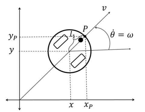
Under the assumption of pure rolling without slipping, the unicycle robot's planar motion can be described by the following kinematic model (see Figure 1):
$\left[\begin{array}{c}\dot{x} \\ \dot{y} \\ \dot{\theta}\end{array}\right]=\left[\begin{array}{cc}\cos \theta & 0 \\ \sin \theta & 0 \\ 0 & 1\end{array}\right]\left[\begin{array}{c}v \\ \omega\end{array}\right]$ (1)
Here, $(x, y)$ denotes the position coordinates of the robot's geometric center in the global frame, $\theta$ represents its orientation (heading angle), $v$ is the linear velocity, and $\omega$ is the angular velocity about the vertical axis.
This kinematic model, often referred to as the nonholonomic unicycle model, encapsulates the fundamental constraint that the robot cannot move sideways. Its control design is particularly challenging because the system is nonlinear and underactuated, meaning it has fewer control inputs than state variables.
This formulation has been extensively employed in the control literature, including classical works such as Samson’s chained form transformations [1], as well as more recent flatness-based methods and geometric control approaches [3, 6].
2.2 Constrained forward point modeling
In many real-world scenarios, such as vision-based navigation or tool-centric tracking, the control objective is not to guide the robot's geometric center ($x, y$), but rather a forwardlocated point $P$, situated along the robot's longitudinal axis at a fixed offset $l_1$. This forward point better represents sensor or effector locations in practical applications [7] (see Figure 1).
Figure 1. Geometric representation of the forward point P and the unicycle mobile robot model
The Cartesian coordinates of point P, expressed as a function of the robot’s configuration, are given by:
$\left[\begin{array}{l}x_P \\ y_P\end{array}\right]=\left[\begin{array}{l}x \\ y\end{array}\right]+l_1\left[\begin{array}{l}\cos \theta \\ \sin \theta\end{array}\right]$ (2)
where, $\theta$ is the robot's orientation and $l_1>0$ is the fixed distance from the robot's center to point $P$.
Differentiating Eq. (2) with respect to time yields the kinematics of the point P:
$\left[\begin{array}{c}\dot{x}_P \\ \dot{y}_P\end{array}\right]=v\left[\begin{array}{c}\cos \theta \\ \sin \theta\end{array}\right]+l_1 \omega\left[\begin{array}{c}-\sin \theta \\ \cos \theta\end{array}\right]$ (3)
where,$v$ and $\omega$ represent the robot’s linear and angular velocities, respectively.
This expression reveals that the forward point’s velocity depends nonlinearly on the robot’s configuration and control inputs. Crucially, it illustrates how turning motions introduce lateral displacements inP , a factor that complicates control and can lead to geometric instability if not properly addressed [8]. The formulation thus motivates the use of differential flatness, where pointP can be directly employed as a flat output, allowing for trajectory planning and control in the task space.
2.3 Differential flatness of the constrained forward point
In the proposed formulation, the Cartesian coordinates of the forward tracking point P are selected as the flat outputs of the system:
$\mathbf{y}_f=\left[\begin{array}{l}x_P \\ y_P\end{array}\right]$ (4)
According to the principles of differential flatness, all system states and control inputs can be algebraically expressed as functions of the flat outputs and their finite-order time derivatives. This enables both trajectory generation and controller design to be conducted within the flat output space, thus simplifying the treatment of nonlinear dynamics.
Following the differential flatness framework introduced in [3], we examine the forward-point kinematics defined by Eqs. (2)-(3). To establish the flatness of the unicycle model with a forward-point output, we begin by differentiating the output expressions:
$\mathbf{y}=\left[\begin{array}{cc}\cos \theta & -\ell_1 \sin \theta \\ \sin \theta & \ell_1 \cos \theta\end{array}\right]\left[\begin{array}{l}v \\ \omega\end{array}\right], \quad \operatorname{det}(\cdot)=\ell_1 \neq 0$. (5)
Since the transformation matrix is always invertible for $\ell_1 \neq 0$, the control inputs $v$ and $\omega$ can be explicitly computed from the flat output and its derivatives:
$\begin{aligned} v & =\dot{x}_P \cos \theta+\dot{y}_P \sin \theta \\ \omega & =\frac{-\dot{x}_P \sin \theta+\dot{y}_P \cos \theta}{\ell_1}\end{aligned}$ (6)
To reconstruct the full system state, we next compute the orientation $\theta$. It is obtained using the flat output’s first and second derivatives. We first define the curvature of the output trajectory [12]:
$\kappa=\frac{\dot{x}_P \ddot{y}_P-\dot{y}_P \ddot{x}_P}{\left(\dot{x}_P^2+\dot{y}_P^2\right)^{3 / 2}}$ (7)
Then, the orientation is recovered by combining geometric and curvature-based expressions. Specifically, the heading angle is given by [12]:
$\theta=\operatorname{atan} 2\left(\dot{y}_P, \dot{x}_P\right)-\arctan \left(\frac{1-\sqrt{1-4 \ell^2 \kappa^2}}{2 \ell \kappa}\right)$ (8)
This expression ensures a smooth and unique recovery of orientation even under significant curvature, improving over simple kinematic backstepping.
Finally, the original position of the chassis center $(x, y)$ is recovered algebraically as:
$\begin{aligned} & x=x_p-\ell \cos \theta \\ & y=y_p-\ell \sin \theta\end{aligned}$ (9)
Hence, every state variable $(x, y, \theta)$ and input $(v, \omega)$ is fully determined from the flat output $\mathrm{y}=\left[\begin{array}{ll}\mathrm{x}_{\mathrm{P}} & \mathrm{y}_{\mathrm{P}}\end{array}\right]^{\mathrm{T}}$ and its derivatives up to second order. The system is therefore differentially flat [3].
This differential-flatness formulation underpins the entire control strategy, the control laws are expressed directly in the flat outputs $\left(x_P, y_P\right)$ rather than in the full nonlinear state vector $(\mathrm{x}, \mathrm{y}, \theta)$, by doing so, the nonlinearities of the unicycle kinematics are effectively decoupled, which simplifies the synthesis of robust and computationally efficient trajectory-tracking controllers, such flatness-based design method-logies are widely recommended in the nonlinear-systems literature, especially for nonholonomic vehicles like unicycle mobile robots [3].
2.4 Tracking error formulation in polar coordinates
To facilitate the synthesis of the fractional-order PID controller, the tracking error between the reference point and the constrained forward point P is transformed into polar coordinates, a technique well-established in the control of unicycle-type robots [9]. This representation enables a decoupled interpretation of the tracking task, separating translational and angular dynamics, which simplifies the design of two independent control channels.
The polar errors are defined as follows:
$\begin{aligned} & \rho=\sqrt{\left(x_r-x_p\right)^2+\left(y_r-y_p\right)^2} \\ & \alpha=\operatorname{atan} 2\left(y_r-y_p, x_r-x_p\right)-\theta\end{aligned}$ (10)
The use of polar coordinates offers a geometric perspective of the control problem and proves particularly effective in handling the nonholonomic constraints of unicycle models.
This representation forms the basis for the control law developed in the next section, allowing independent regulation of both position and heading errors through fractional-order feedback dynamics.
3.1 Motivation for fractional-order control
Fractional-order control (FOC) has emerged as a powerful paradigm for improving the robustness and precision of control systems, particularly in the presence of nonlinearities, unmodeled dynamics, and disturbances. Unlike classical PID controllers, the FOPID controller introduces two additional degrees of freedom, the integral order $\lambda$ and the derivative order $\mu$ which allows for a richer and more flexible tuning of the closed-loop response [4, 5].
When applied to trajectory tracking tasks involving nonholonomic systems, FOPID controllers have been shown to enhance performance by leveraging the memory and hereditary characteristics inherent to fractional calculus [10, 11, 13]. These properties enable smoother control actions and improved convergence, especially when dealing with real-world uncertainties.
In the context of the differentially flat unicycle system established in Section 2, where the flat output is defined as the coordinates of the forward tracking point P, we adopt a fractional-order control approach for regulating the system. The control design is based on the tracking errors expressed in polar coordinates, as previously defined in Eq. (10), by expressing the control problem in these coordinates, the translational and rotational dynamics are effectively decoupled, thereby simplifying the design of the FOPID controller. This transformation forms the basis for the next subsection, in which the control law is formally derived using fractional-order error dynamics.
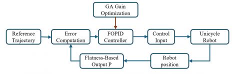
A visual overview of the proposed control architecture is provided in Figure 2, highlighting the key components of the flatness-based FOPID controller and its interaction with the robot model.
Figure 2. Block diagram of the flatness-based FOPID control architecture
3.2 FOPID control law formulation
Building upon the polar error formulation defined in Eq. (10), we develop an FOPID controller to regulate the robot’s translational and rotational motion through the control of the tracking errors. $\rho$ and $\alpha$. The resulting control inputs are given by:
$v(t)=k_p^\rho \rho(t)+k_i^\rho \mathcal{I}^{L_\rho}[\rho(t)]+k_d^\rho \mathcal{D}^{\mu_\mu}[\rho(t)]$ (11)
$\omega(t)=k_p^\alpha \alpha(t)+k_i^\alpha \mathcal{I}^{\alpha^2}[\alpha(t)]+k_d^\alpha \mathcal{D}^{\mu^\mu}[\alpha(t)]$ (12)
where,
This FOPID structure generalizes the classical PID controller by introducing two additional tuning parameters $\lambda$ and $\mu$, offering greater flexibility in shaping the frequency response and dynamic behavior of the [4, 5].
Novelty of the Proposed Control Approach
The originality of our contribution lies in the integration of FOPID control within a differentially flat framework for a constrained forward-tracking point on a unicycle-type mobile robot:
Compared to previous studies on classical PID or linear feedback designs, our method addresses the dynamic coupling and nonlinearity introduced by the constrained point P, and enhances robustness against perturbations through the memory effect of fractional calculus. The recent findings in [13] support the application of FOPID to nonholonomic robots, especially under uncertainties.
3.3 Discrete Grünwald–Letnikov approximation
To implement the FOPID controller in discrete time, we adopt the Grünwald–Letnikov (GL) approximation. This approach is well-suited for real-time control applications due to its recursive structure and ability to approximate fractional derivatives and integrals using finite history data.
The discrete-time approximations of the fractional integral and fractional derivative of a signal $e(t)$ are expressed as:
$\mathcal{I}^\lambda[e]\left(t_k\right) \approx h^\lambda \sum_{j=0}^{N-1} \omega_j^{(\lambda)} e\left(t_{k-j}\right)$, (13)
$\mathcal{D}^\mu[e]\left(t_k\right) \approx h^{-\mu} \sum_{j=0}^{N-1} \omega_j^{(\mu)} e\left(t_{k-j}\right)$, (14)
where, $h$ is the sampling time, $N$ is the memory length [14], and $\omega_j^{(v)}$ are the fractional weights computed recursively by:
$\omega_0^{(v)}=1, \quad \omega_j^{(v)}=\left(1-\frac{v+1}{j}\right) \omega_{j-1}^{(v)}, \quad j \geq 1$ (15)
In our implementation, the tracking errors $\rho$ and $\alpha$ are stored in First-In-First-Out (FIFO) queues of fixed length $N=$ 500, updated at each sampling instant. This memory length corresponds to a 1 -second historical window under the simulation time step $h=0.01 s$. While the general rule-ofthumb proposed in [14] suggests $N \approx 5 / h$. The buffered error history enables the controller to capture the long-memory effects characteristic of fractional-order dynamics, leading to smoother and more adaptive control responses.
This discrete approximation method strikes a favorable trade-off between numerical accuracy and computational load, and has proven effective in recent applications of FOPID controllers in both mobile robotic systems and industrial processes [5, 14].
3.4 Fractional Lyapunov stability analysis
Let the polar-error vector be:
$\mathbf{e}(t)=\left[\begin{array}{l}\rho(t) \\ \alpha(t)\end{array}\right], \quad$ with $\mu, \lambda \in(0,1)$ (16)
Using the FOPID control laws defined in Eqs. (11)–(12), and applying the small-angle approximations, the error dynamics become [1]:
$\dot{\rho}=-v+v_r, \quad \dot{\alpha}=\omega-\omega_r$ (17)
This results in the following closed-loop system in the Caputo fractional-order sense [15]:
$D^1 \mathbf{e}+k_p \mathbf{e}+k_i D^{-\lambda} \mathbf{e}+k_d D^\mu \mathbf{e}=0$ (18)
where, $D^v$ denotes the fractional derivative of order $v$, and $k_p, k_i, k_d>0$ are positive definite diagonal gain matrices.
We propose the following Lyapunov functional [16]:
$V(\mathbf{e})=\frac{1}{2} \mathbf{e}^{\top} \mathbf{e}+\frac{c}{2} \mathbf{e}^{\top} D^{-\lambda} \mathbf{e}, \quad$ with $0<c<2 \min \left(k_d\right)$ (19)
Taking the derivative of order $1-\mu$ of $V$, we obtain:
$\begin{gathered}D^{1-\mu} V=-\mathbf{e}^{\top}\left(k_p \mathbf{e}+\left(k_d-\frac{c}{2}\right) D^\mu \mathbf{e}+k_i D^{-\lambda} \mathbf{e}\right) \leq-\eta\|\mathbf{e}\|^2 \\ \eta=\frac{1}{2} \min \left(k_p\right)>0\end{gathered}$ (20)
By invoking the fractional comparison lemma of Li and Chen [15], inequality (20) implies the following bound on the polar error:
$\|\mathbf{e}(t)\| \leq C E_{1-\mu}\left(-\eta t^{1-\mu}\right), \quad t \geq 0$ (21)
where, $E_{1-\mu}($.$)$ denotes the Mittag–Leffler function. This establishes fractional asymptotic stability of the system. Both components of the error vector converge to zero over time, and the control inputs $(v, \omega)$ remain bounded for all admissible reference trajectories.
Remark 1.
Inequality (20) holds because both $D^\mu e$ and $D^{-\lambda} e$ are $L_2-$ inner-product positive operators when $0<\lambda, \mu<1$ [17].
Remark 2.
Due to Brockett’s non-integrability condition [1], global exponential stabilization of nonholonomic systems with smooth static feedback is impossible. Therefore, Mittag–Leffler convergence is the strongest achievable result under smooth fractional-order control in continuous time.
4.1 Simulation setup
The simulation environment was implemented in MATLAB, modeling a unicycle-type mobile robot using a discrete-time FOPID controller. The reference trajectory is a circular path of radius $R=2 \mathrm{~m}$, centered at the origin, with the tracking point $P$ located $l_1=0.5 m$ ahead of the robot center.
The system was simulated for a duration of $T=40 s$, with a sampling period of $h=0.01 s$, resulting in $N=500$ memory steps used for fractional-order error buffering. The maximum linear and angular velocities were bounded as: $v_{\max }=1 \mathrm{~m} / \mathrm{s}$, $\omega_{\max }=1.5 \mathrm{rad} / \mathrm{s}$.
4.2 Parameter tuning via Genetic Algorithm (GA)
To determine the optimal gains of the FOPID controller, a Genetic Algorithm (GA) was used to minimize the following objective function:
$J=\int_0^T\left[\rho^2(t)+\alpha^2(t)+\beta_v v^2(t)+\beta_\omega \omega^2(t)\right] d t$ (22)
where,
GA Settings:
As a result of the optimization process, the following FOPID parameters were selected for simulation:
$k_p^\rho=2.0, k_i^\rho=0.4, k_d^\rho=0.2$,
$k_p^\alpha=4.5, \quad k_i^\alpha=0.5, \quad k_d^\alpha=0.3$,
$\lambda_\rho=0.9, \mu_\rho=0.8$
$\lambda_\alpha=0.9, \mu_\alpha=0.8$
Bounds keep the GA well-conditioned and consistent with actuator limits and discretization. We set $k_p, k_i, k_d \in[0,10]$ after a coarse sweep indicated diminishing returns beyond $\approx 8$ 10 together with more frequent v -saturation and derivative noise; negative gains were excluded. Fractional orders were limited to $\lambda, \mu \in[0.7,1.0]$ because smaller orders require much longer GL memory or yield slower transients at fixed ($h=0.01 s, N=500$). The chosen ranges align with reported practice in [5, 13]. The gains were obtained via GA; to check sensitivity, we re-ran the GA under several initial pose offsets and headings (within the same operating range) on the same trajectory family, and the optimizer consistently returned similar gain sets. For transparency and reproducibility, we therefore adopt the gain set produced for the initial conditions used in the reported simulations and use that same set throughout, which yields accurate tracking with smooth, unsaturated control inputs near sharp curves.
4.3 Trajectory tracking performance
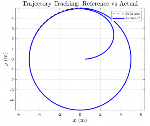
Figure 3 illustrates the trajectory tracking performance of the constrained point $P$. The robot was commanded to follow a circular reference path, using the proposed flatness-based FOPID controller.
As shown in Figure 3, the trajectory tracking is highly accurate. The robot quickly converges to the reference path with no visible overshoot or divergence. The initial deviation visible at the start of the motion is rapidly compensated, and the constrained point $P$ closely follows the planned circular curve. This performance confirms the effectiveness of fractional-order control in handling the nonlinear kinematics of unicycle-type robots while preserving smoothness in tracking behavior.
Figure 3. Reference trajectory vs actual trajectory using the flatness-based FOPID controller
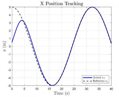
The performance is particularly notable given the nonholonomic constraints, which typically complicate point tracking. Thanks to the differential flatness formulation, the controller operates in a transformed space where the tracking point dynamics are directly accessible. The result is a clean, stable trajectory, validating both the control law and its numerical implementation, Figure 4 illustrates the time evolution of the x -coordinate for the constrained point $P$, comparing the actual trajectory $x_P(t)$ with the reference trajectory $x_r(t)$.
The controller exhibits fast transient convergence during the initial phase (first 10 seconds), followed by excellent tracking accuracy as the trajectory progresses. The slight initial deviation is effectively corrected without overshoot instability, demonstrating the memory and adaptive benefits of fractional-order dynamics.
Figure 4. Tracking performance of the $x_P$ position using the flatness-based FOPID controller
Once stabilized, the actual $x_P$ closely follows the sinusoidal reference path with negligible phase lag and minimal steady-state error. This performance confirms the controller’s ability to regulate the translational dynamics of the nonholonomic system even under complex trajectory profiles.
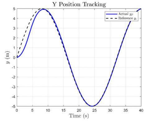
The results further validate the appropriateness of using fractional orders $\lambda_\rho=0.9, \mu_\rho=0.8$, as well as gain values tuned via Genetic Algorithm optimization, as outlined in Section 4.2. and Figure 5 illustrates the tracking performance of the $y$-coordinate of the forward constrained point $P$, comparing the actual output $y_P(t)$ to the reference path $y_r(t)$.
Figure 5. Time evolution of the $y_P$ position under the flatness-based FOPID controller
The trajectory shows a consistent convergence behavior. While an initial transient offset is observed, it is rapidly attenuated demonstrating the controller’s strong corrective dynamics. This early discrepancy is attributable to the inertia of the constrained point $P$, which lies ahead of the robot body and thus magnifies initial heading misalignments.
Once aligned, the system accurately tracks the sinusoidal reference with smooth variations and no observable oscillations or overshoot. This result confirms the FOPID controller’s effectiveness in handling both the nonlinearities of the unicycle model and the memory characteristics of the tracking error dynamics.
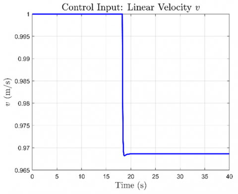
The smoothness is also due to the fractional orders $\lambda_\rho=0.9$, $\mu_\rho=0.8$, which modulate the derivative and integral memory windows in the angular error correction channel. Figure 6 presents the evolution of the linear velocity control input $v(t)$ generated by the FOPID controller during the trajectory tracking task.
Figure 6. Linear velocity command $v(t)$ over time under flatness-based FOPID control
This control signal remains nearly constant at its saturation limit $v_{\max }=1.0 \mathrm{~m} /$ during the initial phase, corresponding to the straight-line acceleration toward the trajectory. A sharp yet bounded drop occurs around $t=40 s$, which coincides with the robot’s curvature adaptation as it aligns itself more accurately with the circular path.
The use of fractional differentiation and integration helps smooth abrupt changes and prevent chattering typical in high-gain integer-order controllers. The memory effect introduced by fractional-order dynamics allows the controller to anticipate the trajectory curvature based on past error history, thus enabling a more adaptive behavior.
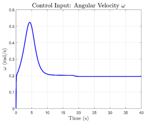
The boundedness of $v(t)$ also aligns with the stability criteria outlined in Section 3.4, ensuring fractional Lyapunov stability and actuator safety. Figure 7 illustrates the time evolution of the angular velocity $\omega(t)$ generated by the proposed flatness-based FOPID controller.
Figure 7. Angular velocity $\omega(t)$ commanded by the FOPID controller
At the beginning of the simulation, the angular velocity increases rapidly to accommodate the sharp change in trajectory curvature required to enter the circular path. The peak value reaches $0.524\ \mathrm{rad} / \mathrm{s}$at time $t=4.3$ seconds. Following this peak, the velocity gradually decreases and stabilizes to a steady-state level of approximately $0.2 \mathrm{rad} / \mathrm{s}$, which is sufficient to maintain circular motion.
This response showcases the controller's ability to deliver smooth and bounded actuation. The absence of overshoot, oscillations, or chattering highlights the damping and memory properties introduced by the fractional-order dynamics. Compared to classical integer-order PID controllers, the FOPID formulation provides better tuning flexibility and allows the system to adapt smoothly to trajectory curvature without introducing instability or aggressive corrections.
The results confirm that the angular control input remains well within the actuation bounds throughout the 40-second maneuver, further supporting the controller’s robustness and suitability for real-world applications.
This work introduced a flatness-based FOPID controller for trajectory tracking of a unicycle mobile robot, applying the control law to a forward-located constrained point to respect the robot’s nonholonomic kinematics. Fractional terms were realized with a discrete Grünwald–Letnikov approximation, allowing memory-aware action that yields smoother responses. Using GA-tuned gains and fractional orders, simulations on a circular path demonstrated high tracking accuracy, smoothly bounded control inputs, and rapid convergence without oscillation or overshoot. A fractional Lyapunov (Mittag–Leffler) analysis further established BIBO stability for the closed loop, underscoring the benefit of embedding fractional dynamics in flatness-based control under realistic actuation limits.
Despite these strengths, several issues remain open. Robustness against unmodeled disturbances, sensor noise, and parameter uncertainty has yet to be verified experimen-tally. Future work will refine the GA procedure into adaptive or online evolutionary tuning, carry out disturbance-rejection and noise-sensitivity tests, and validate the scheme on physical robot platforms. Finally, the method will be exten-ded to cooperative multi-robot formations via decentralized flatness-based coordination laws with integrated collision avoidance.
This work has been supported by the LACoSERE Laboratory of University of Laghouat. The authors gratefully acknowledge the laboratory's financial and technical assistance throughout the course of this research. This support has been instrumental in enabling the progress and development of the work presented here.
|
$\left(x_P, y_P\right)$ |
Cartesian coordinates of the tracking point $P[\mathrm{~m}]$ |
|
$\left(x_r, y_r\right)$ |
Reference trajectory coordinates [m] |
|
$v(t)$ |
Linear velocity of the robot [m/s] |
|
$\omega(t)$ |
Angular velocity of the robot [rad/s] |
|
$\rho(\mathrm{t})$ |
Distance error between point $P$ and the reference [m] |
|
$\alpha(\mathrm{t})$ |
Heading error angle between robot and trajectory tangent [rad] |
|
$\mathrm{l}_1$ |
Distance from the robot center to point $P$ [m] |
|
$T$ |
Total simulation duration [s] |
|
$h$ |
Sampling period [s] |
|
$N$ |
Number of memory steps in fractional-order buffer |
|
$k_p^\rho, k_i^\rho, k_d^\rho$ |
FOPID gains for $\rho$ error |
|
$k_p^\alpha, k_i^\alpha, k_d^\alpha$ |
FOPID gains for $\alpha$ error |
|
$\omega_j^{(v)}$ |
Grünwald–Letnikov weights for order $v$ |
|
$u(t)$ |
Control input vector $[v(t), \omega(t)]^T$ |
|
$P$ |
Tracking point on the robot (constrained point) |
|
$e(t)$ |
General control error signal |
|
Greek symbols |
|
|
$\theta$ |
Orientation (heading angle) of the robot [rad] |
|
$\lambda_\rho, \mu_\rho$ |
Fractional integral and derivative orders for $\rho$ |
|
$\lambda_\alpha, \mu_\alpha$ |
Fractional integral and derivative orders for $alpha$ |
|
$\mathcal{I}^{\ell}$ |
Fractional integral of error $e(t)$ |
|
$\mathcal{D}^\mu$ |
Fractional derivative of error $e(t)$ |
[1] Samson, C. (2002). Control of chained systems application to path following and time-varying point-stabilization of mobile robots. IEEE Transactions on Automatic Control, 40(1): 64-77. https://doi.org/10.1109/9.362899
[2] Petrov, P., Kralov, I. (2024). Exponential trajectory tracking control of nonholonomic wheeled mobile robots. Mathematics, 13(1): 1. https://doi.org/10.3390/math13010001
[3] Fliess, M., Lévine, J., Martin, P., Rouchon, P. (1995). Flatness and defect of non-linear systems: Introductory theory and examples. International Journal of Control, 61(6): 1327-1361. https://doi.org/10.1080/00207179508921959
[4] Podlubny, I. (1998). Fractional Differential Equations. An introduction to fractional derivatives, fractional differential equations, to methods of their solution and some of their applications (Vol. 198). Elsevier.
[5] Monje, C.A., Chen, Y., Vinagre, B.M., Xue, D., Feliu, V. (2010). Fractional-Order Systems and Controls: Fundamentals and applications. London: Springer London. https://doi.org/10.1007/978-1-84996-335-0
[6] Bloch, A.M., Krishnaprasad, P.S., Marsden, J.E., Murray, R.M. (1996). Nonholonomic mechanical systems with symmetry. Archive for Rational Mechanics and Analysis, 136(1): 21-99. https://doi.org/10.1007/BF02199365
[7] Sharma, R.S., Shukla, S., Karki, H., Shukla, A., Behera, L., KS, V. (2019). Dmp based trajectory tracking for a nonholonomic mobile robot with automatic goal adaptation and obstacle avoidance. In 2019 International Conference on Robotics and Automation (ICRA), Montreal, QC, Canada, pp. 8613-8619. https://doi.org/10.1109/ICRA.2019.8793911
[8] Wang, Y., Miao, Z., Zhong, H., Pan, Q. (2015). Simultaneous stabilization and tracking of nonholonomic mobile robots: A Lyapunov-based approach. IEEE Transactions on Control Systems Technology, 23(4): 1440-1450. https://doi.org/10.1109/TCST.2014.2375812
[9] Siegwart, R., Nourbakhsh, I.R., Scaramuzza, D. (2011). Introduction to Autonomous Mobile Robots (2nd ed.). MIT Press, Cambridge.
[10] Husnain, S., Abdulkader, R. (2023). Fractional order modeling and control of an articulated robotic arm. Engineering, Technology & Applied Science Research, 13(6): 12026-12032. https://doi.org/10.48084/etasr.6270
[11] Al-Mayyahi, A., Wang, W., Birch, P. (2016). Design of fractional-order controller for trajectory tracking control of a non-holonomic autonomous ground vehicle. Journal of Control, Automation and Electrical Systems, 27(1): 29-42. https://doi.org/10.1007/s40313-015-0214-2
[12] do Carmo, M.P. (1976). Differential Geometry of Curves and Surfaces. Prentice-Hall, Englewood Cliffs.
[13] Aguilar-Pérez, J.I., Duarte-Mermoud, M.A., Velasco-Villa, M., Castro-Linares, R. (2025). Fractional order tracking control of a disturbed differential mobile robot. PLoS One, 20(5): e0321749. https://doi.org/10.1371/journal.pone.0321749
[14] Tricaud, C., Chen, Y. (2010). An approximate method for numerically solving fractional order optimal control problems of general form. Computers & Mathematics with Applications, 59(5): 1644-1655. https://doi.org/10.1016/j.camwa.2009.08.006
[15] Li, Y., Chen, Y., Podlubny, I. (2009). Mittag–Leffler stability of fractional order nonlinear dynamic systems. Automatica, 45(8): 1965-1969. https://doi.org/10.1016/j.automatica.2009.04.003
[16] Sontag, E.D. (2009). Stability and feedback stabilization. In Encyclopedia of Complexity and Systems Science, New York, NY, pp. 8616-8630. https://doi.org/10.1007/978-0-387-30440-3_515
[17] De Luca, A., Oriolo, G., Vendittelli, M. (2002). Control of wheeled mobile robots: An experimental overview. Ramsete: Articulated and Mobile Robotics for Services and Technologies, 270: 181-226. https://doi.org/10.1007/3-540-45000-9_8