Elhoussein Elouardi*![]() | Lhoussain El Bahir
| Lhoussain El Bahir![]() | Ismail Lagrat
| Ismail Lagrat![]() | Younes Adnani
| Younes Adnani![]() | Brahim Elouardi
| Brahim Elouardi![]() | Omar Mouhib
| Omar Mouhib![]()
© 2025 The authors. This article is published by IIETA and is licensed under the CC BY 4.0 license (http://creativecommons.org/licenses/by/4.0/).
OPEN ACCESS
This paper proposes a robust control strategy to enhance the stability, speed tracking accuracy, and disturbance rejection of electric vehicles (EVs) powered by Permanent Magnet Synchronous Motors (PMSMs). The strategy aims to design a fuzzy Proportional-Integral (PI) controller based on Takagi-Sugeno (TS) fuzzy modeling, integrating a Line Integral Lyapunov Function (LILF) with an H∞ control approach to ensure both robustness and optimal dynamic performance. The controller gains are optimized using Linear Matrix Inequality (LMI) technique, enabling adaptability under various operating conditions. Simulation results demonstrate the superior performance of the proposed LILF-based controller compared to Linear Quadratic Function (LQF) and traditional PI controllers. Specifically, it achieves a rise time of 6 ms, zero overshoot, and no steady-state error, while effectively eliminating vibrations. In contrast, the PI controller exhibits a 21% overshoot and a steady-state error of 0.24. Additionally, the proposed strategy shows strong resilience to external disturbances, contributing to smoother and more energy-efficient EV operation. The suggested controller offers a useful and efficient solution for real-world EV propulsion systems requiring high precision and robustness.
electric vehicle, Line Integral Lyapunov Function (LILF), PMSM Motor, fuzzy control, Linear Matrix Inequality (LMI), H∞ Performance
Transport makes a considerable impact on global energy demand and greenhouse gas emissions, accounting for one-third of total energy consumption and approximately 20% of global emissions [1-5]. In response to escalating environmental concerns, EVs have emerged as a viable and sustainable alternative [6-8]. EVs offer several advantages, including environmental friendliness, reduced noise levels, higher efficiency, and lower energy consumption compared to conventional internal combustion engine vehicles [9]. As a result, many countries are increasingly adopting EVs to mitigate environmental impacts [7, 10]. In fact, according to the International Energy Agency (IEA), 2023 witnessed the fastest growth on record, with global EV sales increasing by 35% to nearly 14 million vehicles. Furthermore, the first quarter of 2024 recorded a 25% year-on-year increase in sales, and projections estimate around 200 million EVs on the road worldwide by 2030 [3, 10].
Despite the technical progress achieved in the EV industry, several challenges persist, particularly in terms of safety and energy management, which hinder the seamless integration of EVs into existing transportation systems [9, 11, 12].
Permanent Magnet Synchronous Motors (PMSMs) have been widely used in electric vehicles (EVs) propulsion system due to their high efficiency, excellent torque performance and smaller size [5, 13]. However, new control strategies are needed to improve the performance of PMSM drive systems in both EVs and hybrid electric vehicles (HEVs) [14].
In order to ensure accurate trajectory tracking under variable road conditions with parameter uncertainties and external load disturbances, robust speed control is essential in EVs driven by PMSMs. To achieve this, Proportional-Integral (PI) controllers have been widely used in the literature due to their balance between simplicity and efficiency. Considerable research has been devoted to improving PI tuning techniques adapted to different system designs, in order to ensure optimal performance under various conditions [14-19]. Nonlinear tuning of PI parameters has been explored to achieve fast response and low overshoot [15] while Fractional-Order PI controllers have shown promising results in PMSM drive applications [16]. Furthermore, advanced methodologies, such as a Zero-Pole elimination (ZPE) method have enhanced the performance of the PMSM drive [17]. Fuzzy logic has also been applied in the study [18] for robust, stable and fast EV powertrain control.
Traditional PI controllers continue to be highly popular due to their simplicity, but they frequently perform poorly in the presence of non-linearities and external disturbances [14]. To overcome these drawbacks, a control method using QLF was presented in the study [19]. While it improved stability, it required solving complex and sometimes overly conservative matrix conditions. To address these issues, this paper proposes a novel control approach based on the LILF function, combined with Takagi-Sugeno (TS) fuzzy modeling and H∞ control, for designing a PI controller for EV speed tracking and disturbance rejection. Unlike QLF method, which requires a common matrix across all subsystems, the LILF method performs local stability analysis for each fuzzy rule and integrates them using fuzzy logic. This approach reduces conservatism, enhances performance, and provides better disturbance handling.
The rest of this paper is structured as follows: Section 2 introduces the proposed methodology, starting with the EV system description and the PMSM modeling, including its TS fuzzy representation. Section 3 focuses on the detailed design of the control strategy, including the stability analysis based on the LILF. The fuzzy PI controller gains are computed by solving a set of constraints formulated as Linear Matrix Inequalities (LMIs). Section 4 discusses the simulation results, highlighting the controller’s effectiveness in terms of tracking precision and robustness. Furthermore, it gives a comparative evaluation with existing methods of the state of the art. Finally, Section 5 concludes the paper by highlighting the main contributions of this work and suggesting perspectives for future research.
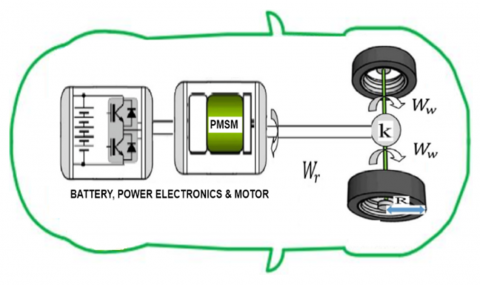
2.1 EV system description
Figure 1 shows the main components of an EV powertrain, including the battery, power electronics, motor, shaft, and wheels.
Figure 1. The powertrain of the electric vehicle
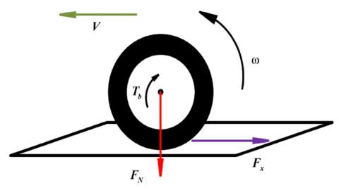
The complete model of vehicle dynamics is nonlinear and highly complex, as it must take into account various factors such as road conditions, aerodynamic drag, etc. Since vehicle motion results from the interaction between each wheel and the road surface, a quarter-vehicle model [20] is selected for this study as shown in Figure 2.
Figure 2. Quarter vehicle model description [20]
Using the fundamental principles of dynamics, the following equations, Eq. (1) and Eq. (2), describe the motion of the system:
$m \frac{d \mathrm{Vx}}{d t}=-F_x$ (1)
$J \frac{d W}{d t}=-T_b+r F_x$ (2)
where m, W, and J denote, respectively, the vehicle mass, the angular velocity, and the wheel inertia. Vx is the longitudinal velocity of the vehicle, Tb is the braking torque, r is the radius of the wheel and Fx denotes the longitudinal friction force. It is known that the force Fx is a natural by-product of the torque generated by the electric motor. According to Coulomb's law, Fx can be represented as the product of the adhesion coefficient of the road $\mu(\lambda)$ and the vertical force FN as follows:
$F_x=\mu(\lambda) F_N=\mu(\lambda) \mathrm{mg}$ (3)
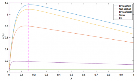
where g is the gravitational acceleration constant. The wheel slip $\lambda=\frac{V_x-r W}{V_x}$ is used to quantify the difference between the vehicle speed and the wheel speed during acceleration or braking [21]. Burckhardt's model [22] is the most widely used to describe the variation of $\mu(\lambda)$ as a function of $\lambda$, due to its simplicity and acceptable accuracy:
$\mu(\lambda)=C 1\left(1-e^{-C 2 \lambda}\right)-C 3 \lambda$ (4)
where the choice of the parameters (Ci; i=1,2,3) characterizes the road type. Figure 3 shows the variation of the adhesion coefficient μ(λ) for different road conditions.
It is known that the longitudinal speed of a vehicle, denoted as $V x$, is a function of the rotational speed of its engine $W r$. Under certain driving conditions, $V x$ can be considered proportional to the engine's rotational speed. This proportional relationship is valid under specific assumptions, including the presence of a direct transmission or a constant gear ratio (as is often the case with automatic gearboxes), an engine operating steadily within its optimal range of revolutions per minute, and negligible mechanical and aerodynamic losses. In such conditions, the vehicle’s speed is directly influenced by the engine speed, the transmission ratio, and the radius of the wheels. The relationship between the vehicle’s longitudinal speed and the engine’s rotational speed can then be expressed as $V x=\mathrm{K} \cdot W r$, where K = R⋅k, R is the wheel radius, and k is the overall gear ratio. This scenario corresponds to a wheel slip value $\mu(\lambda)$ ≤ 0.2, as illustrated by the dashed pink box in Figure 3.
Figure 3. Variation of adhesion coefficient μ(λ)
In this context, our main objective is to control the PMSM motor to achieve an angular speed $W_r{ }^d$, that matches the desired speed profile $V_r{ }^d$ commanded by the driver.
2.2 Permanent magnet synchronous motor modeling
Electric vehicles rely heavily on rotating machines, particularly PMSMs, which are preferred for their high efficiency [23]. This subsection explains the dynamics of a PMSMs. The equations describing the stator voltage components in the direct-quadrature (dq) reference frame for a PMSM are defined as follows:
$\left\{\begin{array}{c}V_q=R_s i_q+L_q \frac{d i_q}{d t}+W_r L_d i_d+W_r \phi_m \\ V_d=R_s i_d+L_d \frac{d i_d}{d t}-W_r L_q i_q\end{array}\right.$ (5)
where $V_q$ and $V_d$ are the voltages in the dq-reference frame, $i_q$ and $i_d$ are the corresponding currents, $R_s$ is the stator winding resistance, $L_q$ and $L_d$ are the inductances in the dqframe, $\phi_m$ is the permanent magnet flux linkage, and $W_r$ is the electrical rotor speed. Applying the fundamental principle of dynamics, the operation of the PMSM can be described as follows:
$\frac{d W_r}{d t}=\frac{-B}{J} W_r+\frac{3 n_p^3 \phi_m}{8 J} i_q-\frac{n_p C_r}{2 J}$ (6)
The electromagnetic torque Ce produced by the PMSM is given by:
$C e=\frac{2 J}{n_p} \cdot \frac{d W_r}{d t}_r+\frac{2 B}{n_p} \cdot W+C_r$ (7)
where B is the damping coefficient, J is the moment of inertia, $n_p$ is the number of magnetic pole pairs, and $C r$ is the load torque. The Ce can be also expressed as [19]:
$C e=\frac{3 n_p}{4}\left[\phi_m i_q+\left(L_q-L_d\right) i_q i_d\right]$ (8)
For a PMSM with surface-mounted magnets, where Lq≈Ld, the system is modeled in the state-space domain as:
$\begin{aligned} {\left[\begin{array}{c}\dot{W_r} \\ \dot{l_q} \\ \dot{l_d}\end{array}\right]=} & {\left[\begin{array}{ccc}\frac{-B}{J} & \frac{3 n_p^3 \phi_m}{8 J} & 0 \\ \frac{-\phi_m}{L_q} & \frac{-R_s}{L_q} & \frac{-L_d}{L_q} W_r \\ 0 & \frac{-L_q}{L_d} W_r & \frac{-R_s}{L_d}\end{array}\right]\left[\begin{array}{c}W_r \\ i_q \\ i_d\end{array}\right] } \\ & +\left[\begin{array}{cc}0 & 0 \\ \frac{1}{L_q} & 0 \\ 0 & \frac{1}{L_d}\end{array}\right]\left[\begin{array}{c}V_q \\ V_d\end{array}\right]+\left[\begin{array}{c}\frac{-n_p C r}{2 J} \\ 0 \\ 0\end{array}\right]\end{aligned}$ (9)
This Eq. (9) can be simplified to:
$\left\{\begin{array}{c}\dot{x}(t)=A(x(t)) x(t)+B u(t)+v(t) \\ y(t)=W_r=\left[\begin{array}{lll}1 & 0 & 0\end{array}\right] x(t)=C x(t)\end{array}\right.$ (10)
where $v(t)$ represents the disturbances of the system that can be modeled as follows:
$v(t)=\left[\begin{array}{c}\frac{-n_p}{2 J} \\ 0 \\ 0\end{array}\right]=\left[\begin{array}{ccc}\frac{-n_p}{2 J} & 0 & 0 \\ 0 & 0 & 0 \\ 0 & 0 & 0\end{array}\right]\left[\begin{array}{c}C r \\ 0 \\ 0\end{array}\right]=D \Psi(t)$ (11)
2.2.1 Takagi–Sugeno Fuzzy Model of the PMSM
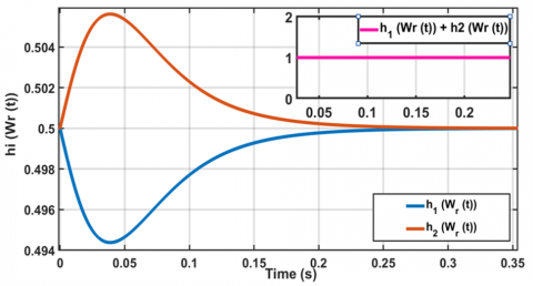
The Takagi–Sugeno (T–S) fuzzy model [24] is widely used to address the nonlinearities inherent in complex systems, such as the PMSM model [25]. Assuming that the scheduling variable $W_r$ in Eq. (8) is bounded between a minimum and a maximum value $W_r{ }^{\min } \leq W_r \leq W_r{ }^{\max }$. In this case, $W_r$ can be expressed as a convex combination:
$W_r(t)=h_1\left(W_r(t)\right) W_r^{\min }+h_2\left(W_r(t)\right) W_r^{\max }$ (12)
where $h_{\mathrm{i}}\left(W_r(t)\right)$ are the weighting functions, defined as follows:
$\left\{\begin{array}{l}h_1\left(W_r(t)\right)=\frac{W_r^{\max }-W_r}{W_r^{\max }-W_r^{\min }} \\ h_2\left(W_r(t)\right)=\frac{W_r-W_r^{\min }}{W_r^{\max }-W_r^{\min }}\end{array}\right.$ (13)
These weighting functions $h_{\mathrm{i}}\left(W_r(t)\right)$ for i=1,2, satisfy the following convexity conditions:
$\sum_{i=1}^2 h_i\left(W_r(t)=1\right.$ and $0 \leq h_i\left(W_r(t) \leq 1, i=1,2\right.$ (14)
Figure 4 illustrates the convexity of the Eq. (14).
Figure 4. Convexity validation of $h_{\mathrm{i}}\left(W_r(t)\right)$ functions
T–S fuzzy logic enables us to represent the nonlinear system described by Eq. (10) as a convex combination of linear sub-models as follows:
$\left\{\begin{array}{c}\dot{x}(t)=\sum_{i=1}^2 h_i\left(W_r(t)\right)\left[A_i x(t)+B_i u(t)+D_i \Psi(t)\right] \\ y(t)=\sum_{i=1}^2 h_i\left(W_r(t)\right) C_i x(t)\end{array}\right.$ (15)
where,
$A_1=\left[\begin{array}{ccc}\frac{-B}{J} & \frac{3 n_p^3 \phi_m}{8 J} & 0 \\ \frac{-\phi_m}{L_q} & \frac{-R_s}{L_q} & \frac{-L_d}{L_q} W_r^{\min } \\ 0 & \frac{-L_q}{L_d} W_r^{\min } & \frac{-R_s}{L_d}\end{array}\right] ;$
$A_2=\left[\begin{array}{ccc}\frac{-B}{J} & \frac{3 n_p^3 \phi_m}{8 J} & 0 \\ \frac{-\phi_m}{L_q} & \frac{-R_s}{L_q} & \frac{-L_d}{L_q} W_r^{\max } \\ 0 & \frac{-L_q}{L_d} W_r^{\max } & \frac{-R_s}{L_d}\end{array}\right] ;$
$B_i=B$ and $D_i=D ; \quad i=1,2$.
The main objective of the proposed control strategy is to enhance the stability, ensure accurate tracking of the desired speed profile $V_x{ }^d$ commanded by the driver, and improve disturbance rejection in the PMSM powered EV. In this framework, the control task consists of adjusting the motor's angular velocity $W_r{ }^d$ so that it corresponds to the desired vehicle speed $V_x{ }^d$. To fulfill these objectives, a fuzzy Proportional-Integral (PI) controller is developed based on Takagi-Sugeno (TS) fuzzy modeling. The approach incorporates a LILF and an $\mathrm{H} \infty$ control framework to guarantee both robustness and high dynamic performance under varying conditions. The control design problem is formulated as an optimization task subject to LMI constraints, which yields to the optimal controller gains.
3.1 Mathematical Lemmas
Lemma. 1 [26]. Let X and Y be two matrices of appropriate dimensions. Then the following inequality holds:
$X^T Y+Y^T X \leq{ }_\gamma^{-1} X^T X+{ }_\gamma Y^T Y$ (16)
Lemma. 2 [19, 27]. Let Z_isj be a matrix of appropriate dimensions, where {i,s,j} =1…r. If Z_isj< 0, then the following global inequality holds:
$\sum_{i=1}^r \sum_{s=1}^r \sum_{j=1}^r Z_{i s j}<0$ (17)
Lemma. 3 [28]. Let Q, R, and S be matrices of appropriate dimensions, where $\mathrm{Q}=\mathrm{Q}^T$ and $\mathrm{R}=\mathrm{R}^T$. The following equivalence holds:
$\left[\begin{array}{cc}Q & S \\ * & R\end{array}\right]<0 \Leftrightarrow\left\{\begin{aligned} R<0 \\ Q-\mathrm{S}^T \mathrm{R}^{-1} S<0\end{aligned}\right.$ (18)
3.2 Stability analysis using the Line Integral Lyapunov Function (LILF)
Typically, the Quadratic Lyapunov Function (QLF) approach, commonly used for stability analysis and stabilization of TS fuzzy models, leads to conditions formulated as LMIs or BMIs (Bilinear Matrix Inequalities). The QLF method involves finding a common matrix $\mathrm{P}=\mathrm{P}^T>0$ that satisfies the stability conditions for all subsystems in the fuzzy model. However, this task can be particularly challenging and may lead to conservative and computationally intensive solutions [29, 30].
To address these limitations, the LILF has been proposed. This function is defined as the integral of a scalar function along the system’s trajectory [31]. Unlike the QLF, the LILF approach performs a local stability analysis for each subsystem individually. The global stability function is then obtained as a fuzzy intersection of these local functions [32], leading to less restrictive and more flexible stability conditions. Consider the following Lyapunov candidate function:
$V(x(t))=2 \oint_{\Gamma(0 ; x)} f(\phi) d \phi$ (19)
Rhee et al. [31] have demonstrated that the Eq. (19) is a Lyapunov function if the following conditions are satisfied:
$\frac{\partial f_m(x)}{\partial x_n}=\frac{\partial f_n(x)}{\partial x_m} ;$ for $n \neq m,\{n, m\}=\{1,2 \ldots n\}$ (20)
where where $\left.f(x(t))=\sum_{i=1}^r h_i(\Theta)\right) P_i x(t)>0$, and $P_i x(t)=(P 0+\sum_{i=1}^r h_j(\Theta) \widehat{P}_i) x(t)$; The diagonal elements change based on the fuzzy sets in the premise of the fuzzy rules [31].
$P 0=P 0^T=\left[\begin{array}{ccccc}0 & h_{12} & h_{12} & \ldots & h_{1 n} \\ * & 0 & h_{23} & \ldots & h_{2 n} \\ * & * & \ddots & \vdots \\ * & * & \ldots & 0\end{array}\right] ;\ \widehat{P}_i=\left[\begin{array}{ccccc}d_{11}{ }^i & 0 & 0 & \ldots & 0 \\ * & d_{22}{ }^i & 0 & \ldots & 0 \\ * & * & \ddots & & \vdots \\ * & * \ldots & & d_{n n}{ }^i\end{array}\right]$
The analysis based on the QLF can therefore be regarded as a special case of the LILF. The following example demonstrates the comparison of the stability regions obtained using LILF and those derived from the QLF.
Example 1. [30] Let us consider the following nonlinear model:
$\dot{x}(t)=\sum_{i=1}^4 h_i\left(W_r(t)\right)\left[A_i x(t)+B_i u(t)\right]$ (21)
where,
$A_1=\left[\begin{array}{ll}-12 & -4 \\ 0.2(7 a-6)+6 a & -6\end{array}\right]$,
$A_2=\left[\begin{array}{ll}-12 & -4 \\ 0.2(7 a-1)+a & -1\end{array}\right]$,
$A_3=\left[\begin{array}{ll}-6 & -4 \\ 0.2(b-6)+6 a & -6\end{array}\right]$,
$A_4=\left[\begin{array}{ll}-6 & -4 \\ 0.2(b-1)+a & -1\end{array}\right]$,
$B_1=\left[\begin{array}{l}0 \\ 1\end{array}\right], \quad B_2=\left[\begin{array}{l}0 \\ 1\end{array}\right], \quad a \in[0 ; 50], \quad b \in[0 ; 80]$
Figure 5 shows the feasibility comparison via LILF and QLF. By analyzing the stability of the system described in Eq. (20), we can note that the QLF, represented by blue asterisks (*), produces more restrictive results compared to the FILF, represented by red diamonds (◊). This result justifies the use of LILF in this study.
Figure 5. Feasibility comparison via (LILF) and (QLF)
3.3 Structure and design of the proposed controller
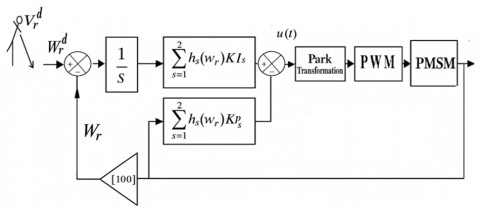
Figure 6 illustrates the structure of the proposed fuzzy PI controller, whose control input u(t) is defined as follows:
$u(t)=-\sum_{s=1}^2 h_s\left(W_r(t)\right)\left[K_{p s} x(t)+K_{I s} \int_0^t\left(W_r-W_r^d\right) d t\right]$ (22)
Figure 6. Structure of the proposed fuzzy controller strategy
Let us consider the H∞ performance criterion related to the tracking error $\mathrm{e}_{\mathrm{c}}(\mathrm{t})$:
$\int_0^{\infty} \mathrm{e}_{\mathrm{c}}^T(\mathrm{t}) \mathrm{e}_{\mathrm{c}}(\mathrm{t}) \mathrm{dt} \leq \gamma^2 \int_0^{\infty} \xi^T(\mathrm{t}) \xi(\mathrm{t}) \xi(\mathrm{t}) \mathrm{dt}$ (23)
To ensure the stability of the fuzzy T-S closed-loop system given in Eq. (10) and to develop a robust controller, the candidate function (LILF) Eq. (19) and the $\mathrm{H} \infty$ criterion Eq. (23) is employed. The controller gains are computed by solving the LMI conditions described in the following theorem:
Theorem: If there exist a symmetric positive definite matrix $X_j, Y_{s j}, K_s$, and scalars $\gamma>0$, such that the following inequality holds:
$\left[\begin{array}{ccc}\Xi_{i s j} & \widehat{D} & X N^T \\ * & -\gamma I & 0 \\ * & * & -I\end{array}\right]<0$ (24)
where $\mathrm{N}=\left[\begin{array}{lll}1 & 0 & 0\end{array}\right]$, and I is the identity matrix with the corresponding dimensions and $\Xi_{i s j}=\widehat{A}_{\imath}^T \mathrm{X}_j+\mathrm{X}_j \widehat{A_{\imath}}-\widehat{B} Y_{s j}- Y_{s j}{ }^T \hat{B}^T$; where $Y_{s j}=K_s \mathrm{X}_j$.
Then the system Eq. (15) is asymptotically stable, and the $H_{\infty}$ performance described in Eq. (22) is guaranteed with attenuation level $\gamma$.
Where $X_j$ and $Y_{s j}$ (thus $\mathrm{Ks}=Y_{s j} X_j^{-1}$ ) can be easily obtained by solving LMI Eq. (23).
Proof: Let's denote the tracking error dynamic:
$\dot{e}_c=W_r-W_r^d$ (25)
Substituting Eq. (20) into Eq. (14) the following augmented system is obtained:
$\left[\begin{array}{c}\dot{x} \\ \dot{e}_c\end{array}\right]=\sum_{i=1}^2 \sum_{i=1}^2 h_i h_s\left[\left[\begin{array}{cc}A_i-B K_{p i} & B K_{I i} \\ M & 0\end{array}\right]\left[\begin{array}{c}x \\ e_c\end{array}\right]+\left[\begin{array}{cc}A_i & D \\ 0 & 0\end{array}\right]\left[\begin{array}{c}W_r{ }^d \\ \Psi\end{array}\right]\right]$ (26)
which can be written as:
$\dot{\hat{x}}(t)=\sum_{i=1}^2 \sum_{s=1}^2 h_i h_s\left[\left(\widehat{A}_l-\widehat{B} K_s\right) x+\widehat{D} \xi(t)\right]$ (27)
where,
$\begin{gathered}\widehat{A}_l=\left[\begin{array}{ll}A_i & 0 \\ \mathrm{M} & 0\end{array}\right] ; \quad \widehat{B}=\left[\begin{array}{l}\mathrm{B} \\ 0\end{array}\right] ; \quad \widehat{\mathrm{D}}=\left[\begin{array}{cc}A_i & D \\ 0 & 0\end{array}\right] ; \\ M=\left[\begin{array}{lll}1 & 0 & 0\end{array}\right] ; \quad K_s=\left[\begin{array}{l}K_{p s} K_{I s}\end{array}\right] ; \quad \xi(t)=\left[\begin{array}{c}W_r{ }^d \\ \Psi\end{array}\right]\end{gathered}$
The goal is to design the controller Eq. (20) such that:
$\checkmark$ The system Eq. (25) globally asymptotically stable.
$\checkmark$ $H_{\infty}$ performances Eq. (21) are satisfied.
To achieve these goals, the $H_{\infty}$ performance related to the tracking error $e_c$ Eq. (21) is combined with Lyapunov candidate function Eq. (18) such as:
$\dot{V}(\hat{x}(\mathrm{t}))+\hat{x}^t(t) M^T \mathrm{M} \hat{x}(\mathrm{t})-\gamma^2 \xi(\mathrm{t})^{\mathrm{T}} \xi(\mathrm{t})<0$ (28)
where M= [10 0].
By replacing the time derivative of $\dot{V}(\hat{x}(\mathrm{t}))$ with its expression, the inequality Eq. (26) becomes:
$\sum_{i=1} \sum_{s=1} \sum_{j=1} h_i h_s h_j \dot{\hat{x}}(\mathrm{t})^T P_j \hat{x}(\mathrm{t})+\hat{x}(\mathrm{t}) \cdot P_j \dot{\hat{x}}(\mathrm{t})+\hat{x}^t(\mathrm{t}) M^T \mathrm{M} \hat{x}(\mathrm{t})-\gamma^2 \xi(\mathrm{t})^{\mathrm{T}} \xi(\mathrm{t})<0$ (29)
For simplicity, thereafter we consider the following notation:
$\sum_{i=1} \sum_{s=1} \sum_{j=1} h_i h_s h_j \dot{\hat{x}}(\mathrm{t})^T=\sum_{i, s, j=1} h_{i s j}$ (30)
Replacing the time derivative of $\dot{\hat{x}}(t)$ in Eq. (26) with its expression, the inequality Eq. (19) becomes:
$\begin{gathered}\sum_{i, s, j=1} h_{i s j}\left[\left(\widehat{A}_l-\widehat{B} K_s\right)+\widehat{D} \xi(t)\right]^T P_j \hat{x}(\mathrm{t})\\+\hat{x}(\mathrm{t}) P_j\left[\left(\widehat{A}_l-\widehat{B} K_s\right) x+\widehat{D} \xi(t)\right]+\hat{x}^t(t) M^T \mathrm{M} \hat{x}(\mathrm{t}) -\gamma^2 \xi(\mathrm{t})^{\mathrm{T}} \xi(\mathrm{t})<0\end{gathered}$ (31)
By applying Lemma. 1 the inequality Eq. (31) can be expressed as follows:
$\sum_{i, s, j=1} h_{i s j} \hat{x}(\mathrm{t})^T\left[\begin{array}{c}P_j\left(\widehat{A_{\imath}}-\widehat{B} K_s\right)^T+\left(\widehat{A_{\imath}}-\widehat{B} K_s\right) P_j+ \\ \gamma^{-2} P_j \widehat{D}^{\mathrm{T}} \widehat{D} P_j+M^T \mathrm{M}\end{array}\right] \hat{x}(\mathrm{t})<0$ (32)
Using Lemma. 2 the system Eq. (26) is globally asymptotically stable; therefore, the system Eq. (15) is asymptotically stable with $H_{\infty}$ performance given in Eq. (23), provided the following conditions are satisfied:
$\begin{gathered}P_j\left(\widehat{A}_l-\widehat{B} K_s\right)^T+\left(\widehat{A}_l-\widehat{B} K_s\right) P_j+\gamma^{-2} P_j \widehat{D}^{\mathrm{T}} \widehat{D} P_j+ M^T \mathrm{M}<0 ;\{\mathrm{i}, \mathrm{s}, \mathrm{j}\}=\{1,2\}\end{gathered}$ (33)
Post- and pre-multiply $X_j$, (where $X_j=P_j^{-1}$ and $Y_{s j}=\mathrm{Ks} X_j$ ), the inequality Eq. (31) can be expressed as:
$\begin{gathered}\widehat{A}_l^T P_j+P_j \widehat{A}_{l i}-\widehat{B}_l^T Y_{s j}-Y_{s j}{ }^T \widehat{B}_l+\gamma^{-2} \widehat{D}^{\mathrm{T}} \widehat{D}+ X_j M^T \mathrm{M} X_j<0 ;\{\mathrm{i}, \mathrm{s}, \mathrm{j}\}=\{1,2\}\end{gathered}$ (34)
Finally, Schur’s complement (Lemma. 3) is applied to Eq. (33) to derive the LMI conditions presented in Eq. (23).
To demonstrate the effectiveness of the proposed control strategy, simulations were conducted on a PMSM motor, whose parameters are listed in Table 1.
Table 1. PMSM and EV parameters [19]
|
Parameters |
Values |
|
Stator resistance |
Rs = 2.875 $\Omega$ |
|
Direct axis inductance |
Ld = 7.5 mH |
|
Quadrature axis inductance |
Lq = 2.5 mH |
|
Moment of inertia |
J = 0.0008 Kg |
|
Coefficient of friction |
f = $10^{-4}$ N.m.s/rad |
|
Flux linkage established by the PMSM |
$\phi_m$ = 0.175 Wb |
|
Maximum PMSM rotor speed |
$W_r^{\max }$ = 1800 rpm |
|
Minimum PMSM rotor speed |
$W_r^{\min }$ = - 1800 rpm |
|
Number of magnetic poles |
$n_p$ = 8 |
Using the lmiterm function of MATLAB to solve the Linear Matrix Inequality (LMI) conditions in Eq. (23) (LMI solving time: < 1 s), the control gains for the fuzzy Proportional-Integral (PI) controller defined in Eq. (21) were obtained as follows:
$\begin{gathered}K P 1=\left[\begin{array}{clc}5.7780 & 11.7586 & 6.4279 \\ 1.3747 & 2.4339 & 14.3841\end{array}\right], \\ K I 1=10^3\left[\begin{array}{l}3.8664 \\ 1.0239\end{array}\right]\end{gathered}$
$\begin{gathered}K P 2=\left[\begin{array}{ccc}5.7780 & 11.7586 & -6.4279 \\ -1.3747 & -2.4340 & 14.3841\end{array}\right], \\ K I 2=10^3\left[\begin{array}{l}3.8664 \\ 1.0239\end{array}\right]\end{gathered}$
These control gains were subsequently implemented in a MATLAB/SIMULINK simulation.
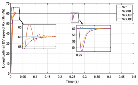
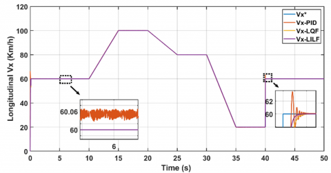
To evaluate the regulation performance of the designed controller, a reference speed profile $V_x^*$ to be tracked is proposed in Figure 7. The response of the proposed approach is then compared with other methods of the state of the art (Figure 7).
Figure 7. Longitudinal EV speed $V_x$
The comparison reveals that our proposed FILF controller outperforms both the traditional PI controller [14] and the QLF approach-based controller developed in [19], in terms of reference speed tracking $V_x^*$ rise time, accuracy, and absence of overshoot. For reference and reuse, the performance metrics of the different controllers are summarized in Table 2.
Table 2. Comparison of PI, QLF and LIFF controllers performs
|
Performs Type |
LIFF |
LQF [19] |
PI [14] |
|
Rise time (s) $10^{-3}$ |
6 |
8 |
10 |
|
Overshoot % |
0 |
0 |
21 |
|
Static error |
0 |
0 |
0.24 |
|
Vibration |
absent |
absent |
exist |
|
Response to disturbances |
good |
fast |
very fast |
Assuming small slip angle values, the motor must rotate at a specific angular speed $W_r{ }^*$ corresponding to the reference longitudinal speed of the vehicle $V_x{ }^*$. Figure 8 shows that $W_r$ follows the same dynamics as $V_x$, scaled by a proportional coefficient.
Figure 8. Motor angular rotation speed $W_r$
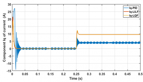
Referring to the currents shown in Figures 9 and 10, it can be observed that the controllers designed using the FILF and QLF approaches produce smoother current waveforms with fewer high-frequency harmonics compared to the traditional PI controller.
Figure 9. Variation of $I_d$ current components versus time
Figure 10. Variation of $I_q$ current components versus time
To quantify the high-frequency harmonics of each controller, the Total Harmonic Distortion (THD) is used as a figure of merit, measuring the number of harmonics present in each current relative to its fundamental component. The lower the THD, the fewer high-frequency harmonics are present in the current. The THD values for different current components are illustrated in Table 3.
Table 3. THD comparison of $I_d$ and $I_q$ currents
|
|
THD (%) |
||
|
LIFF |
LQF |
PI |
|
|
$I_d$ |
6.53 |
18.8 |
28.1 |
|
$I_q$ |
9.45 |
18.7 |
33.4 |
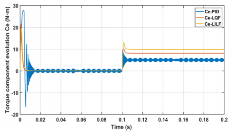
It can be noted that the FILF approach achieves the lowest THD values for both the $I_d$ and $I_q$ components, outperforming both the QLF approach and the conventional PI controller. Furthermore, the FILF approach results in lower current consumption compared to the QLF method. This improvement directly impacts the electromagnetic torque generated by the machine as illustrated in Figure 11. The reduction of harmonics leads to a smoother torque output and consequently less vibration.
Figure 11. Torque variation $C_e$ versus time
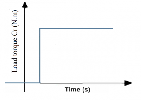
It is well known that external disturbances can degrade system performance and may even cause instability. To evaluate the robustness of the proposed controller, a disturbance in the form of a step load torque ($C_r$= 10 N.m) shown in Figure 12 is applied to the system at a time of (t = 0.25s). Figures 7 and 8 demonstrate that the FILF-based controller responds faster than the QLF-based controller, while the PI controller exhibits speed oscillations due to this disturbance.
Figure 12. Load torque profile $C_r$
The application of this disturbance forces the motor to generate a stronger electromagnetic torque to counteract its effect, resulting in an increased current draw. This explains the variations observed in the current components in Figures 9 and 10, as well as the torque fluctuations in Figure 11 at the moment the disturbance is applied.
Robustness against parametric uncertainties, such as changes in stator resistance ($Rs$) due to temperature changes after the application of load torque disturbances, is particularly important in vehicular applications, where sudden load changes (for example, caused by passengers entering or exiting) can occur. This is a crucial aspect that needs to be taken into account in the design of the controller. In particular, the control system must quickly compensate for any disturbance in order to maintain vehicle speed which is an essential condition for ensuring high dynamic performance. To evaluate the robustness of our proposed LILF controller against stator resistance disturbances, a test is performed under resistance variations of ($Rs$ ± 20%). The simulation results shown in Figure 13 demonstrate the ability of the controller to effectively reject these parametric perturbations while maintaining system stability and confirm that, thanks to the $H \infty$ control effect, the proposed controller is able to effectively handle these parametric uncertainty variations.
Figure 13. EV speed tracking under Rs variation
Driving under real road conditions requires the vehicle to vary its speed based on factors such as traffic signs or driver intent. Therefore, the controller must possess sufficient dynamic capability to adjust the reference speed $V_x^*$ according to varying scenarios. Consequently, the PMSM motor must produce torque appropriate to each new driving condition.
From the comparison shown in Figure 14, it is evident that the FILF controller tracks the reference speed $V_x^*$ with greater accuracy, particularly during sudden speed changes (t=40 s) compared to the other controllers.
Figure 14. Tracking longitudinal EV speed $V_x^*$
This work introduces a fuzzy PI control strategy for electric vehicle speed regulation based on a Line Integral Lyapunov Function (LILF) combined with an H∞ control framework. Unlike traditional PI or QLF-based designs, the proposed approach offers enhanced robustness, precise speed tracking, and smoother current and torque profiles, without the need for frequent gain adjustments.
Beyond demonstrating technical superiority through simulation, this method contributes significantly to advancing EV control systems by providing an efficient, low-maintenance solution that improves both vehicle performance and energy efficiency. These features make the controller especially well-suited for next-generation electric mobility applications, where adaptability and reliability are paramount.
Future work will focus on real-time validation via hardware-in-the-loop (HIL) simulations and experimental testing. Furthermore, integration of AI-based control techniques and computer vision will be explored to further enhance adaptability and vehicle autonomy.
The datasets used and/or analysed during the current study is available from Mr. El Houssein El Ouardi through elhoussein.elouardi1@uit.ac.ma.
[1] Saldaña, G., San Martin, J.I., Zamora, I., Asensio, F.J., Oñederra, O. (2019). Electric vehicle into the grid: Charging methodologies aimed at providing ancillary services considering battery degradation. Energies, 12(12): 2443. https://doi.org/10.3390/en12122443
[2] Nguyen, H.H., Kim, J., Hwang, G., Lee, S., Kim, M. (2019). Research on novel concept of hybrid electric vehicle using removable engine-generator. In 2019 IEEE Vehicle Power and Propulsion Conference (VPPC), Hanoi, Vietnam, pp. 1-5. https://doi.org/10.1109/VPPC46532.2019.8952405
[3] IEA. (2024). Global EV Outlook 2024, IEA, Paris. https://www.iea.org/reports/global-ev-outlook-2024.
[4] Elouardi, E., Sellak, L., El Mokhi, C., Adnani, Y., Idkhajine, L., Mouhib, O. (2024). Lateral control for autonomous vehicles utilizing an ANN-based controller. In 2024 10th International Conference on Optimization and Applications (ICOA), Almeria, Spain Almeria, Spain, pp. 1-5. https://doi.org/10.1109/ICOA62581.2024.10754161
[5] Gobbi, M., Sattar, A., Palazzetti, R., Mastinu, G. (2024). Traction motors for electric vehicles: Maximization of mechanical efficiency—A review. Applied Energy, 357: 122496. https://doi.org/10.1016/j.apenergy.2023.122496
[6] Farajnezhad, M., Kuan, J.S.T.S., Kamyab, H. (2024). Impact of economic, social, and environmental factors on electric vehicle adoption: A review. Eídos, 17(24): 39-62. https://doi.org/10.29019/eidos.v17i24.1380
[7] Dua, R., Almutairi, S., Bansal, P. (2024). Emerging energy economics and policy research priorities for enabling the electric vehicle sector. Energy Reports, 12: 1836-1847. https://doi.org/10.1016/j.egyr.2024.08.001
[8] Mohammed, A., Saif, O., Abo-Adma, M., Fahmy, A., Elazab, R. (2024). Strategies and sustainability in fast charging station deployment for electric vehicles. Scientific Reports, 14(1): 283. https://doi.org/10.1038/s41598-023-50825-7
[9] Hossain, M.S., Kumar, L., El Haj Assad, M., Alayi, R. (2022). Advancements and future prospects of electric vehicle technologies: A comprehensive review. Complexity, 2022(1): 3304796. https://doi.org/10.1155/2022/3304796
[10] Gottumukkala, R., Merchant, R., Tauzin, A., Leon, K., Roche, A., Darby, P. (2019). Cyber-physical system security of vehicle charging stations. In 2019 IEEE Green Technologies Conference (GreenTech), Lafayette, USA, pp. 1-5. https://doi.org/10.1109/GreenTech.2019.8767141
[11] Arévalo, P., Ochoa-Correa, D., Villa-Ávila, E. (2024). A systematic review on the integration of artificial intelligence into energy management systems for electric vehicles: Recent advances and future perspectives. World Electric Vehicle Journal, 15(8): 364. https://doi.org/10.3390/wevj15080364
[12] Ouyang, T.C., Wang, C.C., Xu, P.H., Ye, J.L., Liu, B.L. (2023). Prognostics and health management of lithium-ion batteries based on modeling techniques and Bayesian approaches: A review. Sustainable Energy Technologies and Assessments, 55: 102915. https://doi.org/10.1016/j.seta.2022.102915
[13] Guo, Y.G., Yu, Y.F., Lu, H.Y., Lei, G., Zhu, J.G. (2024). Enhancing performance of permanent magnet motor drives through equivalent circuit models considering core loss. Energies, 17(8): 1837. https://doi.org/10.3390/en17081837
[14] Kong, L.T., Zhang, H.X., Zhang, T.Z., Wang, J.Y., Yang, C.H., Zhang, Z. (2024). Adaptive control parameter optimization of permanent magnet synchronous motors based on super-helical sliding mode control. Applied Sciences, 14(23): 10967. https://doi.org/10.3390/app142310967
[15] Wu, Z.H., Li, G.S., Zhu, Y., Tian, G.Y., Lu, K. (2010). A new nonlinear pi controller of permanent magnet synchronous motor. In 2010 Second International Conference on Intelligent Human-Machine Systems and Cybernetics, Nanjing, China, pp. 99-102. https://doi.org/10.1109/IHMSC.2010.32
[16] Thakar, U., Joshi, V., Vyawahare, V. (2017). Design of fractional-order PI controllers and comparative analysis of these controllers with linearized, nonlinear integer-order and nonlinear fractional-order representations of PMSM. International Journal of Dynamics and Control, 5: 187-197. https://doi.org/10.1007/s40435-016-0243-0
[17] Hsieh, M.F., Chen, N.C., Ton, T.D. (2019). System response of permanent magnet synchronous motor drive based on SiC power transistor. In 2019 IEEE 4th International Future Energy Electronics Conference (IFEEC), Singapore, pp. 1-6. https://doi.org/10.1109/IFEEC47410.2019.9015197
[18] Khanh, P.Q., Anh, H.P.H. (2022). Improved PMSM speed control using fuzzy pi method for hybrid active and reactive power control approach. In International Conference on Green Technology and Sustainable Development, Da Nang City, Vietnam, pp. 345-356. https://doi.org/10.1007/978-3-031-19694-2_31
[19] Elouardi, E., Mouhib, O., Bentaleb, A., Ouardi, B.E., Lassioui, A., Fadil, H.E. (2023). Cruise control system of electric vehicle powered by pmsm motor using ts fuzzy approach. In International Symposium on Automatic Control and Emerging Technologies, Kenitra, Morocco, pp. 726-735. https://doi.org/10.1007/978-981-97-0126-1_64
[20] Tang, Y.G., Zhang, X.Y., Zhang, D.L., Zhao, G., Guan, X.P. (2013). Fractional order sliding mode controller design for antilock braking systems. Neurocomputing, 111: 122-130. https://doi.org/10.1016/j.neucom.2012.12.019
[21] Abzi, I., Kabbaj, M.N., Benbrahim, M. (2020). Robust adaptive fractional-order sliding mode controller for vehicle longitudinal dynamic. In 2020 17th International Multi-Conference on Systems, Signals & Devices (SSD), Monastir, Tunisia, pp. 1128-1132. https://doi.org/10.1109/SSD49366.2020.9364239
[22] Burckhardt, M. (1993). Fahrwerktechnik: Radschlupf-regelsysteme: Reifenverhalten, zeitablaeufe, messung des drehzustands der raeder, Anti-Blockier-System (ABS), theorie hydraulikkreislaeufe, Antriebs-Schlupf-Regelung (ASR), Theorie Hydraulikkreislaeufe, elektronische Regeleinheiten, Leistungsgrenzen, ausgefuehrte Anti-Blockier-Systeme und Antriebs-Schlupf-Regelungen. Vogel.
[23] Huang, Q., Huang, Q.H., Guo, H.C., Cao, J.C. (2023). Design and research of permanent magnet synchronous motor controller for electric vehicle. Energy Science & Engineering, 11(1): 112-126. https://doi.org/10.1002/ese3.1316
[24] Takagi, T., Sugeno, M. (1985). Fuzzy identification of systems and its applications to modeling and control. IEEE Transactions on Systems, Man, and Cybernetics, SMC-15(1): 116-132. https://doi.org/10.1109/TSMC.1985.6313399
[25] Ounnas, D., Chenikher, S., Bouktir, T. (2013). Tracking control for permanent magnet synchronous machine based on Takagi-Sugeno fuzzy models. In 2013 Eighth International Conference and Exhibition on Ecological Vehicles and Renewable Energies (EVER), Monte Carlo, Monaco, pp. 1-5. https://doi.org/10.1109/EVER.2013.6521548
[26] Chang, X.H., Liu, Y. (2022). Quantized output feedback control of AFS for electric vehicles with transmission delay and data dropouts. IEEE Transactions on Intelligent Transportation Systems, 23(9): 16026-16037. https://doi.org/10.1109/TITS.2022.3147481
[27] Dahmani, H., Pagès, O., El Hajjaji, A., Daraoui, N. (2013). Observer-based tracking control of the vehicle lateral dynamics using four-wheel active steering. In 16th International IEEE Conference on Intelligent Transportation Systems (ITSC 2013), he Hague, Netherlands, pp. 360-365. https://doi.org/10.1109/ITSC.2013.6728258
[28] Zoulagh, T., El Aiss, H., Tadeo, F., El Haiek, B., Barbosa, K.A., Hmamed, A. (2024). Gain-scheduled energy-to-peak approach for vehicle sideslip angle filtering. Symmetry, 16(12): 1627. https://doi.org/10.3390/sym16121627
[29] Saenz, J.M., Tanaka, M., Tanaka, K. (2019). Relaxed stabilization and disturbance attenuation control synthesis conditions for polynomial fuzzy systems. IEEE Transactions on Cybernetics, 51(4): 2093-2106. https://doi.org/10.1109/TCYB.2019.2957154
[30] Houili, R., Hammoudi, M.Y., Benbouzid, M., Titaouine, A. (2023). Observer-based controller using line integral lyapunov fuzzy function for TS fuzzy systems: Application to induction motors. Machines, 11(3): 374. https://doi.org/10.3390/machines11030374
[31] Rhee, B.J., Won, S. (2006). A new fuzzy Lyapunov function approach for a Takagi–Sugeno fuzzy control system design. Fuzzy Sets and Systems, 157(9): 1211-1228. https://doi.org/10.1016/j.fss.2005.12.020
[32] Vafamand, N. (2020). Global non-quadratic Lyapunov-based stabilization of T—S fuzzy systems: A descriptor approach. Journal of Vibration and Control, 26(19-20): 1765-1778. https://doi.org/10.1177/1077546320904817