Priti V. Kale![]() | Narendra M. Kandoi
| Narendra M. Kandoi![]() | Aniket K. Shahade*
| Aniket K. Shahade*![]() | Disha S. Wankhede
| Disha S. Wankhede![]() | Madhura Phadke
| Madhura Phadke![]() | Priyanka V. Deshmukh
| Priyanka V. Deshmukh![]()
© 2025 The authors. This article is published by IIETA and is licensed under the CC BY 4.0 license (http://creativecommons.org/licenses/by/4.0/).
OPEN ACCESS
The work presented here gives a novel approach for detecting liver tumours from medical images. The proposed approach is the combination of the latest segmentation and classification techniques that results in early detection of liver tumours with higher accuracy. The methodology applies three phases, the first is the application of anisotropic diffusion filtering that enhances the image quality without disturbing the structural information. After filtering, the second phase makes use of the U-Net architecture and attention-based transformers (U-TransNet) segmentation model for precisely detecting the boundary delineation and tumour detection. The results show Intersection over Union (IoU) as 98%, and dice scores are 99.01%. The third phase in the proposed method applies a support vector machine optimised using a bio-inspired whale optimisation algorithm. The results measured using parameters like accuracy, recall, precision, and F1-score are close to 99%, considering class imbalance effectively in early stages. Comparative analysis in this study validated that the performance of this is better in high-end and advanced methods in segmentation as well as classification techniques. The proposed system has better performance over existing and therefore has a potential of accurate diagnostic of liver tumors for proper treatment of patients.
liver tumor detection, anisotropic diffusion filtering, U-Net with attention-based transformer, support vector machine (SVM), whale optimization algorithm (WOA)
The liver is one of the body's largest internal organ, located on the right side of the abdomen beneath the ribcage. Growth of liver cells in abnormal fashion above or within the liver can form a mass known as a liver tumor, signalling an underlying liver disease. The liver is susceptible to various diseases, including cirrhosis, hepatitis, and liver cancer [1]. Over the past two decades, the course of cirrhosis and liver cancer have collectively contributed to an estimated total of approximately 50 million deaths worldwide on an annual basis each year.
Metastatic liver cancer typically occurs when cancer spreads to the liver from other affected organs, or vice versa [2]. In such cases, the cancer cells present in the liver typically originate from the primary tumor site elsewhere in the body. Since this clearly indicates cancer progression, doctors usually classify it as advanced cancer of stage 4. Common cancers that frequently metastasize to the liver include colorectal, stomach, lung, pancreatic, breast, melanoma, and esophageal. In most instances, patients with liver metastases tend to develop tumors in both lobes of the liver [3].
1.1 Liver cancer: Cholangiocarcinoma and metastatic disease
Cholangiocarcinoma, a severe form of liver cancer, originates in the bile ducts. As the second most common primary hepatobiliary tumor, its global prevalence has been rising. Cholangiocarcinoma can be classified as intrahepatic (within the liver) or extrahepatic (outside the liver), but both types are collectively termed bile duct cancer due to their origin [4].
While numerous liver diseases exist, this study focuses on metastatic liver cancer and cholangiocarcinoma, both of which are life-threatening conditions.
1.2 Diagnostic challenges and advances in liver imaging
Computed Tomography (CT) is the preferred imaging modality for liver cancer due to its high lesion-to-liver contrast and non-ionising radiation benefits [5]. However, liver segmentation—a critical step in diagnosis—faces challenges such as:
•Scale diversity (varying tumour sizes)
•Complex backgrounds (overlapping tissues)
•Unclear tumour boundaries
•Low contrast in organ density
Accurate segmentation is essential for improving medical assessment and research outcomes [6]. Early and precise detection of cancer in the liver can definitely significantly reduce the rates of mortality and enhance the survival of the patient. Unfortunately, due to late diagnosis, liver disease remains the third leading cause of cancer-related deaths [7].
1.3 Limitations of current classification methods
Existing computerized tumor classification approaches often fail to accurately identify early-stage disease characteristics [8]. While deep learning (DL) networks show potential for classification, their computational demands make them impractical for time-sensitive clinical use. Alternatively, shape-based strategies leveraging historical data offer a promising solution [9].
1.4 The role of AI in liver segmentation
Deep learning through the use of AI can accelerate the formation of probabilistic segmentation models, normally called as PSMs, assisting medical analysis. However, despite these advancements, clinical validation of AI-generated PSMs remains essential to ensure reliability [10]. Additionally, evaluating the clinical feasibility of automated liver segmentation—including the time required for clinically acceptable results—is crucial for real-world implementation [11].
Intensity-based strategies are widely recognised for their rapid implementation, particularly in zone growth, tiering, and threshold-based approaches [12]. However, these methods are predominantly semi-automatic, making them susceptible to noise and often requiring manual intervention when handling complex constraints. While they demonstrate significant improvements in segmentation accuracy when combined with machine learning (ML) techniques [13], most ML-based approaches still rely on manually designed features, which substantially limits their precision.
This limitation has helped in significant advancements not only in convolutional neural networks (CNNs) but also in other deep learning methods and the fully convolutional network (FCN) provides a prominent solution for image classification at pixel-level [14]. Also, the Deep learning techniques have been proved to be far more accurate than conventional ML-based methods. Yet both these architectures, the FCN and U-Net, have notable inherent drawbacks. The FCN-based approach many times fails to produce reliable results for liver segmentation both in case of single-network or cascaded training [15]. The primary reason is due to the fact that pixel-level analysis have a tendency to overlook subtle visual cues [16]. On the other hand, U-Net is efficient but its feature maps remains unrefined till the final convolution step. Additional challenges like vanishing gradients and repeated subsampling leading to the progressive degradation in features is found in deeper U-Net architectures which ultimately reduces output quality [17]. Category imbalance further compounds these issues, introducing errors and poorly defined boundaries in certain liver regions.
Although 3D networks benefit from enhanced z-axis information, memory constraints complicate slice selection, limiting their practicality [18]. While existing methods perform well in many automated liver segmentation scenarios, their accuracy and robustness remain insufficient for direct clinical application, hindering widespread adoption.
To address these challenges, our proposed U-TransNet introduces two major advancements compared to existing U-Net variants such as ResUNet and Attention-UNet. While ResUNet improves feature extraction through residual connections, it often suffers from increased model complexity and limited ability to capture long-range dependencies. Similarly, Attention-UNet enhances focus on salient regions but still relies heavily on local contextual information, which restricts its performance in cases of small or obscured liver lesions. In contrast, U-TransNet integrates the strengths of U-Net with Transformer-based global self-attention, allowing the model to simultaneously preserve fine structural details and capture long-range dependencies across the CT volumes. This dual capability enables more accurate boundary delineation, robust detection of small lesions, and improved generalization across diverse imaging conditions, thereby overcoming the primary shortcomings of existing U-Net variants.
Recent advances in deep learning have significantly improved liver segmentation from CT scans through various innovative approaches. The MCFA-UNet architecture addresses edge feature loss by employing multiscale feature extraction via parallel convolution paths and dual attention mechanisms, while attention gates reduce semantic gaps between encoder-decoder paths [19]. Automated level set methods enhance segmentation through pre-processing techniques, particularly improving tumor identification for earlier diagnosis [20-22]. CNN-based models using 3×3 kernels with ReLU activation and SoftMax classification have demonstrated effective binary classification [23], while transfer learning approaches combining SVM with NH-SVM variants show improved target domain adaptation [24]. The APESTNet framework integrates histogram equalisation with Mask-RCNN for precise segmentation while preventing overfitting [25], and hybrid ResUNet architectures combine ResNet and UNet advantages for better ROI extraction. Comparative studies evaluating CNN versus SVM performance on clinical samples reveal their respective strengths, and advanced 3D approaches like the 3D-SDBN-ESO model leverage Gaussian filtering, CLAHE pre-processing, and seagull optimisation to effectively capture liver anatomy. These diverse methodologies collectively represent significant progress in liver image analysis, though challenges remain in clinical implementation.
Accurate liver segmentation must address vascular structures and achieve complete lesion inclusion, yet existing methods face significant challenges. The liver’s proximity to adjacent organs with similar CT values complicates tumor analysis, while poorly defined boundaries between healthy and diseased tissue further obscure tumor margins. Variability in tumor size, shape, and location across CT images exacerbates these difficulties. Although current techniques have made progress, developing a fully automated segmentation system remains challenging due to inconsistent intensity variations between liver and lesion tissues, differences in contrast, and variable scanner resolutions. These limitations pose a major obstacle in precise tumor delineation and classification. Medical Images that are available through CT and MRI often have noise and artefacts that reduce the accuracy of segmentation and classification models. Existing filtering method either tend to over-smooth the images and thereby lose critical details or underperform in the process of noise removal. Thus, this work proposes a novel hybrid model with an aim to overcome the limitations of the existing approaches and improve segmentation and classification of liver cancer tumors.
Many liver detection systems rely heavily on hand-engineered features, which are limited in capturing complex structures of the liver. The use of deep learning has improved feature extraction but lacks robustness in handling small, early lesions that are often missed. Also, traditional segmentation techniques, including thresholding and region-growing algorithms, struggle with precise boundary delineation of liver tissues due to the proximity of other abdominal organs. This leads to misclassification and inaccurate detection, especially when distinguishing between healthy tissue and early pathological signs. Furthermore, current models face optimization challenges, with sub-optimal tuning of deep learning architectures, leading to underperformance when measured as classification accuracy. Summary of Recent Advances in Liver Segmentation and Classification is shown in Table 1.
Table 1. Summary of recent advances in liver segmentation and classification
|
Reference |
Methodology |
Key Contributions |
Limitations |
|
[18] |
MCFA-UNet |
Multiscale feature extraction, dual attention mechanisms, reduced encoder-decoder semantic gaps |
Edge feature loss in minimal feature extraction |
|
[19] |
Automated level sets |
Improved tumor region identification, early diagnosis support |
Semi-automatic, requires manual intervention |
|
[20] |
CNN (3×3 kernel + ReLU) |
Effective binary classification via SoftMax |
Limited to binary classification, lacks 3D context |
|
[21] |
TL-based SVM + NH-SVM |
Enhanced target domain adaptation, superior classification |
Dependency on paired labels |
|
[22] |
APESTNet (Mask-RCNN + HE) |
Precise segmentation, overfitting prevention |
Computationally intensive |
|
[23] |
Hybrid ResUNet |
Combined ResNet-UNet advantages for ROI extraction |
Limited validation on complex tumors |
|
[24] |
CNN vs. SVM comparison |
Empirical evaluation of classifier performance |
Small sample size (20 cases) |
|
[25] |
3D-SDBN-ESO |
Gaussian/CLAHE preprocessing, seagull optimization |
High memory requirements |
|
Proposed Work |
Novel Hybrid Model |
Addresses intensity variation, unclear boundaries, and lesion diversity |
Validation pending on clinical datasets |
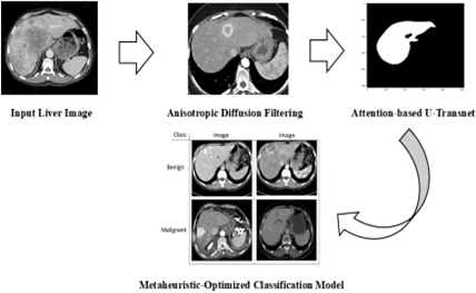
Liver tumor detection through medical imaging, particularly in its early stages, faces significant challenges. Medical Imaging techniques like CT and MRI often introduce noise and artifacts that compromise the accuracy of segmentation and classification models. To address the issues of noise and artefacts in medical images, the proposed method incorporates advanced noise reduction algorithms using anisotropic diffusion filtering (refer to Figure 1). This method is better than the traditional filtering as it can suppress noise effectively still preserving the intricate structures of liver tissues that are important for accurate detection. The enhanced image clarity sets the foundation for more precise segmentation and classification, overcoming over-smoothing limitations seen in earlier approaches. To address the inaccurate segmentation of liver boundaries, the proposed method integrates an Attention-based U-TransNet, which performs the initial segmentation, capturing key liver regions. With its attention mechanism, the transformer layer refines this by focusing on the boundaries and critical regions where early lesions might occur, even if they are small or obscured by noise. The integration of these ensures both macro-level segmentation and fine boundary precision, making it more accurate for early detection than existing models. Thus, the proposed method robustly capture spatial hierarchies, provides long-range attention while handling coarse segmentation, identifying fine liver abnormalities and distinguishing them from nearby tissues.
Figure 1. Proposed flow diagram
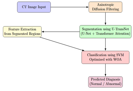
Figure 2 presents the detailed system architecture of the proposed framework, illustrating how segmentation, feature extraction, and classification modules interact. To enhance classification accuracy and overcome the imbalance in early-stage disease detection, we propose a metaheuristic-optimised classification model. A support vector machine (SVM) classifier is tuned using the Whale Optimisation Algorithm (WOA). WOA improves on the standard grid or random search techniques by intelligently exploring the hyperparameter space, leading to optimal model performance. Furthermore, cost-sensitive learning is incorporated to handle class imbalance, assigning higher weights to minority (early-stage disease) samples, thus ensuring they are not under-represented during training. The classification process begins by using the fused feature vector from the earlier step. The SVM classifier is optimised using WOA, which iteratively searches for the best kernel parameters. The combination of noise-resilient preprocessing, hybrid segmentation with attention mechanisms, and metaheuristic optimisation-based classification promises higher segmentation precision, robust feature extraction, and improved classification of early liver disease, making it a significant advancement over current techniques.
Figure 2. Comprehensive system architecture showing the interaction between preprocessing, segmentation, feature extraction, and classification modules
3.1 Anisotropic diffusion filtering
Anisotropic diffusion (Perona–Malik diffusion) is a process in which the image noise is decreased without removing the essential details of the image content for proper image interpretation. Magnetic resonance images normally have noise, and therefore, to remove it without damaging image details, an anisotropic diffusion filter is proposed using Eq. (1).
$\partial I /_{\partial t}=\operatorname{div}(c(x, y, t) \nabla I)=\nabla_C . \nabla I+c(x, y, t) \Delta$ (1)
where I is the original image, the gradient operator is denoted by ∇, Laplacian operator is given by ∆, the divergence operator is donated by div(…) and the coefficient of diffusion is given by c(x,y,t).
In medical image segmentation, enhancing tissue contrast is critical for accurate analysis. As a first pre-processing step, we employ anisotropic diffusion filtering on the original CT images to reduce noise while preserving structural boundaries. This advanced filtering technique offers significant advantages over conventional Gaussian blurring by maintaining edge sharpness during the smoothing process. The method operates through an iterative diffusion process governed by the partial differential Eq. (2):
$\begin{aligned} I_{t+1} & =I_t+\lambda\left(c N_{x, y} \nabla_N\left(I_t\right)+c S_{x, y} \nabla_S\left(I_t\right)\right. \\ & \left.+c E_{x, y} \nabla_E\left(I_t\right)+c W_{x, y} \nabla_W\left(I_t\right)\right)\end{aligned}$ (2)
where the original image is I, the number of iterations carried out is given by t. The diffusion coefficients in the four directions (North (N), West (W), South (S) and East (E)) are indicated by cN,cW,cS, and cE respectively. The following Eqs. (3)-(6) are for anisotropic diffusion:
$c N_{x, y}=\exp \left(-\left\|\nabla_N(I)\right\|^2 / k^2\right)$ (3)
$c S_{x, y}=\exp \left(-\left\|\nabla_S(I)\right\|^2 / k^2\right)$ (4)
$c E_{x, y}=\exp \left(-\left\|\nabla_E(I)\right\|^2 / k^2\right)$ (5)
$c W_{x, y}=\exp \left(-\left\|\nabla_W(I)\right\|^2 / k^2\right)$ (6)
In anisotropic diffusion, the k and λ are two parameters that regulate the level of smoothing, with larger values leading to smoother images, but the edges are not retained as much.
To evaluate how robust the anisotropic diffusion preprocessing is, we performed a sensitivity analysis by testing different values of the edge-stopping parameter (k), the time step (λ), and the number of iterations (N). Specifically, we tested k values of 5, 10, 20, and 40; λ values of 0.05, 0.10, 0.15, and 0.25; and N values of 5, 10, 20, and 40. For each combination of these parameters, we measured segmentation performance using the Dice coefficient, Intersection over Union (IoU), and Mean Squared Error (MSE). Key findings from this analysis are discussed in Section 4.4.
3.2 Anisotropic diffusion filtering
Medical image segmentation typically processes 3D volumetric data x ∈ ℝ^(D×H×W×C). Here spatial dimensions are represented as D, H, W and channel depth is donated by C which is used to generate pixel-wise label maps of matching resolution. Conventional U-Net architectures process this input through sequential encoding and decoding stages, extracting hierarchical features while maintaining spatial resolution. However, these traditional approaches often struggle to capture extensive contextual relationships across medical volumes. Our proposed architecture addresses this limitation by strategically incorporating attention mechanisms throughout the U-shaped network’s encoder and decoder pathways. The enhanced design combines convolutional layers' local feature extraction capabilities with transformer modules' global self-attention mechanisms. This synergistic integration improves modelling of anatomical relationships across different scales while preserving precise spatial details, ultimately achieving more accurate segmentation of complex tissue structures in medical imaging.
Image sequentialization: For 3D medical image processing, we implement volume tokenization by partitioning the input tensor x$\in $ℝD×H×W×C into non-overlapping cubic patches of size P×P×P. This transformation reshapes the volumetric data into a sequence of flattened patch vectors $\left\{x_p^i \in \mathbb{R}^{\wedge^{\mathrm{P}^3} \cdot \mathrm{C}} \mid \mathrm{i}=1, \ldots, \mathrm{~N}\right\}$, where N = (D×H×W)/P³ represents both the total number of patches and the sequence length for subsequent processing. Following established practices in vision transformer architectures, this pacification step serves as the fundamental operation for converting the spatial 3D medical image into a sequence suitable for transformer-based processing, while maintaining all original voxel information through the flattened vector representation.
Patch embedding: Our patch embedding process transforms the vectorised image patches bold x to the p into a d-dimensional latent space through a trainable in-line projection, where p denotes patch size and c represents input channels. To preserve critical spatial information, we augment these patch embeddings with learned positional encodings formulated as Eq. (7):
${{z}_{0}}=\left[ x_{1}^{p}E;x_{2}^{p}E;\cdots ;x_{N}^{p}E \right]+{{E}^{pos}}$ (7)
where, $\mathbf{E}\in {{\mathbb{R}}^{\left( {{P}^{3}}\cdot C \right)\times {{d}_{enc}}}}$ is the patch embedding projection, and $\mathbf{E}^{p o s} \in \mathbb{R}^{N \times d_{\mathrm{enc}}}$ denotes the position embedding.
A standard Transformer layer contains two primary components: The first is Multi-head Self-Attention mechanism (MSA) and second is Multi-Layer Perceptron block (MLP) which are given using Eqs. (2) and (3). Consequently, the l-th layer output zₗ is computed using Eqs. (8) and (9) as:
$\mathbf{z}_{\ell }^{\text{ }\!\!'\!\!\text{ }}=\text{MSA}\left( \text{LN}\left( {{\mathbf{z}}_{\ell -1}} \right) \right)+{{\mathbf{z}}_{\ell -1}}$ (8)
${{\mathbf{z}}_{\ell }}=\text{MLP}\left( \text{LN}\left( \mathbf{z}_{\ell }^{\text{ }\!\!'\!\!\text{ }} \right) \right)+\mathbf{z}_{\ell }^{\text{ }\!\!'\!\!\text{ }},$ (9)
Our framework employs layer normalization (LN(⋅)) to process the encoded image representation zₗ. Departing from conventional pixel-wise segmentation, we reformulate medical image analysis as a mask classification task. Central to our approach are learnable d-dimensional 'organ query' vectors, each representing potential anatomical structures in a given image. Using a fixed set of N organ queries (where N ≫ K, with K being the true number of target classes), the model partitions the image into N candidate regions before assigning appropriate class labels. This design choice, inspired by recent advances in set prediction architectures, deliberately over-generates candidate regions to reduce false negative detections while maintaining computational efficiency. Consider d_dec as the dimension of the object queries, the dot product between the initial green queries ${{\mathbf{P}}^{0}}\in {{\mathbb{R}}^{N\times {{d}_{dec}}}}$ and the embedding the last block feature of the U-Net as $\mathbf{F}\in {{\mathbb{R}}^{D\times H\times W\times {{d}_{dec}}}}$that computes the coarse predicted segmentation map: With ddec as the dimension of the object queries predicted coarse segmentation map can be calculated by the dot product of ${{\mathbf{P}}^{0}}\in {{\mathbb{R}}^{N\times {{d}_{dec}}}}$(the initial organ queries) and $\mathbf{F}\in {{\mathbb{R}}^{D\times H\times W\times {{d}_{dec}}}}\text{ }\!\!~\!\!\text{ }$(U-Net last block feature ) as in Eq. (10):
${{\mathbf{Z}}^{0}}=g\left( {{\mathbf{P}}^{0}}\times {{\mathbf{F}}^{\top }} \right)$ (10)
The activation function g(⋅) combines sigmoid nonlinearity with a 0.5 threshold for binarization, chosen over SoftMax to accommodate overlapping classes in our datasets. The Transformer decoder progressively refines organ queries to improve the initial prediction through multiple layers, each comprising: (1) a self-attention mechanism (MSA block) that captures inter-query relationships, and (2) a cross-attention module that integrates localized, multi-scale CNN features. This dual-path design synergistically combines the Transformer's global contextual understanding with CNN's precise spatial localization capabilities, enabling comprehensive feature representation while preserving anatomical details. The cross-attention mechanism specifically allows each query to dynamically attend to relevant spatial regions in the CNN feature maps, facilitating accurate boundary delineation for overlapping structures.
Our method includes simultaneous training of both decoders namely CNN and Transformer. At the t-th layer $\mathrm{P}^t \in \mathbb{R}^{N \times d_{\text {dec }}}$ represent the refined organ queries and concurrently the U-net feature at intermediate stage is mapped to a d_dec-dimensional feature space represented by F to simplify cross-attention computations. Also, multi-scale CNN topographies can be anticipated as $\mathcal{F}\in {{\mathbb{R}}^{\left( {{D}_{t}}{{H}_{t}}{{W}_{t}} \right)\times {{d}_{dec}}}}$, when the number of upsampling blocks line up with the number of Transformer decoder layers. In this ${{D}_{t}},{{H}_{I}}$, and ${{W}_{I}}$ represents t-th upsampling block spatial dimensions in the feature map. Further, the organ queries at $t+1$-th layer are refined by cross-attention with Eq. (11):
${{\mathbf{P}}^{\nu +1}}={{\mathbf{P}}^{l}}+\text{Softmax}\left( \left( \mathbf{{P}'}{{\mathbf{w}}_{q}} \right){{\left( {{\mathcal{P}}^{\nu }}{{\mathbf{w}}_{k}} \right)}^{\top }} \right)\times \mathcal{F}{{\mathbf{w}}_{v}}$ (11)
where the r-th query topographies are updated using linear projection so as to obtain queries for the subsequent layers by means of the weight matrix $w_q \in R^{\left(d_{d_e} e^{\mathrm{i} \times d_4}\right.}$. The U-Net feature, F, is likewise restructured into keys and values with ${{w}_{k}}\in {{R}^{{{d}_{d}}_{es}{{x}_{k}}}}$ and ${{w}_{v}}\in {{R}^{{{d}_{d}}_{oc}{{x}_{d}}}}$ that are parametric weight matrices. A residual path is used for this restructuring of P following earlier works [25]. Next, a attention refinement as coarse-to-fine is attempted to improve the segmentation accuracy.
Our approach incorporates a coarse-to-fine refinement strategy through a novel mask attention module within the Transformer decoder, specifically designed to enhance small target segmentation in medical images. The module leverages coarse predictions from previous stages to guide subsequent refinements by constraining the cross-attention method to focus primarily on probable foreground regions. This attention masking operation, formulated as A' = A ⊙ M + A (where A is the original attention map and M is the binarized mask from the preceding stage), progressively reduces background interference while preserving the Transformer's global contextual understanding. The iterative application of this mechanism enables precise boundary delineation, particularly for small anatomical structures, by successively refining the region of interest while maintaining computational efficiency through spatially-constrained attention computation. This dual advantage of focused local refinement and preserved global context represents a significant improvement over conventional coarse-to-fine approaches in medical image segmentation.
Concretely, the coarse level mask prediction and the organ queries are initially set as Z0 and P0 respectively followed by the iterative refinement process. At the r-th iteration coarse prediction Z' and the current organ query features P^' are used to calculate the masked cross-attention for refinement of P(+1) for the iterations in the later stages. The calculation includes the current coarse prediction ZI into the affinity matrix as specified in Eqs. (12) and (13):
$\begin{gathered}\mathrm{P}^{\mathrm{N}+1}=\mathrm{P}^{\mathrm{N}}+ \operatorname{Softmax}\left(\left(\mathrm{P}^r \mathrm{w}_q\right)\left(\mathcal{F} \mathrm{w}_k\right)^{\top}+h\left(\mathrm{Z}^r\right)\right) \times \mathcal{F} \mathrm{w}_e\end{gathered}$ (12)
where,
$h\left(\mathbf{Z}^{\prime}(i, j, s)\right)= \begin{cases}0 & \text { if } \mathbf{Z}^l(i, j, s)=1 \\ -\infty & \text { otherwise }\end{cases}$ (13)
The coordinate indices (i,j,s) define the spatial constraints for our cross-attention mechanism, forcing it to operate exclusively within foreground regions while completely suppressing background interference. Through an iterative update scheme that simultaneously optimizes both organ queries and their associated mask predictions, our Transformer decoder progressively enhances segmentation accuracy across multiple refinement stages. As detailed in Algorithm 1, this cyclic process continues until completion at iteration t=T, where T corresponds precisely to the total number of decoder layers, ensuring comprehensive feature integration throughout the network's depth.
In Fine segmentation updated organ queries ${{\text{P}}^{T}}$ is obtained after decoding the final iteration which can be mapped to the final refined binarized segmentation map ${{\text{Z}}^{T}}$ with the dot product of U-Net's last block feature $\text{F}$. Each binarized mask is linked with one semantic class using a linear layer of weight matrices. ${{\text{w}}_{fc}}\in {{\mathbb{R}}^{d\times K}}$ is used to project the refined organ embedding ${{\text{P}}^{T}}$ to the output class logits $\text{O}\in {{\mathbb{R}}^{N\times K}}$ using the Eqs. (14) and (15):
$\text{O}={{\text{P}}^{T}}{{\text{w}}_{{{f}_{c}}}}$ (14)
$\overset{}{\mathop{y}}\,=argma{{x}_{k=0,1,\ldots ,K-1}}O$ (15)
where k is the label index. The final class labels associated with the refined predicted masks ${{\text{Z}}^{T}}$ is $\hat{y} \in \mathbb{R}^N$.
Transformer hyperparameters: The Transformer module within U-TransNet was implemented with 4 encoder–decoder layers. Each multi-head self-attention (MSA) block employed 8 attention heads, each with an embedding dimension of 64, yielding a total hidden size of 512. The feed-forward network within each Transformer block had an intermediate dimension of 2048 with GELU activation. Positional encodings were learned and added to the patch embeddings of dimension 128 before entering the encoder. Layer normalization was applied before each attention and feed-forward block. Dropout with a probability of 0.1 was used throughout to reduce overfitting. These settings were selected after pilot hyperparameter tuning to balance segmentation accuracy with computational efficiency.
3.3 SVM with WOA
Whale Optimization Algorithm (WOA) is a new type of metaheuristic intelligent optimization algorithm proposed by Mirjalili and Lewis. It searches for the best possible solution by mimicking the ‘‘spiral bubble network’’ search strategy that is used humpback whales. The algorithm has the advantages of few adjustment parameters, simple operation, and easy understanding. The WOA mainly involves the following optimization steps: surround prey, spiral predation, and search for prey.
During cooperative hunting, humpback whales employ a strategic encircling behavior to capture prey. Once an individual identifies the optimal hunting position, the entire pod converges toward this location. The overall process is mathematically modeled in our optimization algorithm with the help of position update equations given as Eqs. (16) and (17), that controls the iterative refinement of search agents in the specified solution space.
$D=\left| CM\text{*}\left( t \right)-M\left( t \right) \right|$ (16)
$M\left( t+1 \right)=M\text{*}\left( t \right)-A\cdot D$ (17)
The optimization framework that is proposed has the position vector of the best solution as M*(t). This position vector is found by iteration t and is dynamically updated whenever superior solution is found. The position of current solution at iteration t is denoted by M(t) and the Euclidean distance (D) is calculated over each iteration as difference between M*(t) and M(t). Eqs. (18) and (19) are for the adaptive coefficient vector A that governs the magnitude and C gives direction of solution updates. These coefficients enable balanced exploration-exploitation tradeoffs throughout the optimization process.
$A=2a\cdot r1-a$ (18)
$C=2r2$ (19)
The parameter a given as $a\text{ }\!\!~\!\!\text{ }=\frac{2t}{maxgen}$, where the current iteration is t and the maximum allowed iterations are maxgen, controls the search intensity decreasing linearly from maximum of 2 to minimum of 0 across iterations carried out. This decay schedule balances exploration and exploitation. Additionally, r₁ and r₂ are randomisation vectors whose elements are uniformly distributed in [0,1], introducing stochastic variability to the search process.
During the search process whale is searcher and prey is required optimum solutiom. As the searcher gradually reaches the optimal solution then variable a decreases accordingly. Also, the coefficient A reduces linearly with the variable a according to Eq. (18). When A is [−1, 1] then subsequent position of the new searcher will be between the current position and the optimal position (optimum solution). The searcher will reach the optimal solution in a spiral way, updating its position according to Eq. (19), and gradually reach to the desired solution.
As the search agent converges toward the optimal solution, the control parameter' ‘a’ decreases linearly with iterations, causing coefficient A to similarly diminish. When A falls within [−1,1], the agent enters an exploitation phase where its next position is constrained to the convex space between its current location and the global optimum. For final convergence, the agent follows a logarithmic spiral trajectory that simultaneously maintains directional momentum toward the solution while progressively tightening the search radius. This dual-phase update strategy combines targeted local search with controlled oscillatory movements, ensuring both solution accuracy and convergence stability throughout the optimization process using Eq. (20).
$M\left( t+1 \right)={D}'\cdot eblcos\left( 2\pi l \right)+M\text{*}\left( t \right)$ (20)
where, ${D}'\text{ }\!\!~\!\!\text{ }=\text{ }\!\!~\!\!\text{ }\left| M\text{* }\!\!~\!\!\text{ }333\text{ }\!\!~\!\!\text{ }\left( t \right)\text{ }\!\!~\!\!\text{ }-\text{ }\!\!~\!\!\text{ }M\left( t \right) \right|$ specify the error in i-th searcher and optimal solution at current position; constant b defines logarithmic spiral shape, and random number l has the range [−1,1]. Humpback whales constantly narrow the search range while moving in spiral manner. Therefore with spiral mode and 50% probability of shifting is assumed and the searcher position is updated according to Eqs. (21) and (22).
$M\left( t+1 \right)=M\text{*}\left( t \right)-A\cdot D$ (21)
$M\left( t+1 \right)=D0\cdot eblcos\left( 2\pi l \right)+M\text{*}\left( t \right)$ (22)
where, ${D}'=\left| M\text{*}\left( t \right)-M\left( t \right) \right|$ is the error between the current optimal solution and the i-th searcher.
Random search capability of Humpback whales can enhance global search capabilities of algorithms. The updated Eq. (23) can be used for searching the solution randomly
$M\left( t+1 \right)={{M}_{rand}}\left( t \right)-A\left| C{{M}_{rand}}\left( t \right)-M\left( t \right) \right|$ (23)
where,$\text{ }\!\!~\!\!\text{ }{{M}_{rand}}$ is a position vector randomly selected from the 353 current population (representing a random whale).
SVM is a novel machine learning approach, proposed by Corinna Cortes and Vapnik in the year 1995, is a generalized linear classifier used for binary classification of data in a supervised learning mode. Over traditional neural networks, SVM has advantage of robustness, versatility, computational simplicity, effectiveness and theoretical support. On the contrary, when it is used for regression prediction or pattern recognition, no uniform standard method is available for the selection of its parameters c and g. In SVM fitting function, a minimum optimization problem and the penalty parameter c is introduced. The parameter c is used to fine-tune the objective function to achieve the balance between the minimum relaxation factor and maximum interval, that is, when the sample data is classified incorrectly, the larger the value of the parameter c, the more complex the algorithm will be, thus classification errors will not occur. However, if the parameter c is set too high, the algorithm’s generalization ability will be weakened, and the empirical risk may not change. On the contrary, a smaller value of parameter c reduces the complexity of the algorithm but increases the algorithm’s empirical risk. As a result, it is necessary to use an intelligent optimization algorithm to find a suitable parameter c, so that the support vector machine can perform better.
Coupling of segmentation and classification: The WOA-based SVM optimization is performed independently of the segmentation network training, i.e., the optimization process is decoupled from the U-TransNet training. First, the segmentation module generates complete binary masks of the liver tumor regions. From these segmentation outputs, we extract shape, texture, and intensity-based features that serve as inputs to the SVM classifier. Thus, the full segmentation output is used to drive feature extraction and classification. The WOA algorithm optimizes the SVM parameters (kernel type, C, and Γ) to maximize classification accuracy on the validation set. This design ensures that improvements in segmentation quality directly contribute to better classification, while keeping the optimization stages modular.
The proposed liver disease detection system was implemented using Python and TensorFlow, with an integrated Keras backend for deep learning model development. The dataset comprised annotated liver CT scans, pre-processed using anisotropic diffusion filtering to enhance image clarity by reducing noise while preserving crucial anatomical structures. The segmentation pipeline utilised a hybrid Attention-based U-TransNet model, combining the strengths of U-Net for capturing macro-level features and a Transformer-based attention mechanism for refining boundary detection and highlighting fine details. The learning rate, batch size and number of attention heads are optimised using Hyperparameter tuning which ensured that the model achieved maximum segmentation accuracy. The system was trained on a high-performance CPU, using a combination of Dice Loss and Binary Cross-Entropy as the loss function, to address class imbalance and focus on lesion-specific areas. The classification component employed a support vector machine (SVM), with feature extraction driven by the segmented outputs. The SVM was optimised using the Whale Optimisation Algorithm (WOA), which dynamically adjusted hyperparameters to enhance classification performance. Precision, recall, and F1-score were computed to evaluate the classifier's robustness, particularly in handling early-stage liver disease samples.
4.1 Dataset description
Liver tumors represent a major global health challenge, ranking as the fifth most common cancer in men and ninth in women, with over 840,000 new cases reported in 2018 alone. The liver's susceptibility to both primary and metastatic tumors creates significant diagnostic complexities due to lesions' variable sizes, indistinct margins, and diverse contrast characteristics in CT imaging. Addressing these challenges, our study leverages the comprehensive DeepLesion dataset - comprising 32,120 contrast-enhanced CT slices from 10,594 scans of 4,427 patients, containing 32,735 annotated lesions with bounding boxes and size measurements - to develop advanced segmentation algorithms capable of handling the full spectrum of lesion types (both hyper- and hypo-dense) encountered in clinical practice. This multi-institutional dataset, curated from seven hospitals and research centres, provides the necessary diversity in tumor morphology and imaging characteristics to train robust models for accurate lesion delineation, a critical step toward improving diagnosis and treatment planning for this prevalent malignancy.
Although DeepLesion is a large-scale and diverse CT dataset that includes various types of lesions across multiple organs, it is not liver-specific. Its inclusion of liver lesions provides valuable samples for training a generalizable model; however, the dataset also contains heterogeneous lesion types from other organs. While this diversity helps the model learn robust feature representations, it introduces the limitation that liver-specific tumor characteristics may not be as comprehensively represented as in dedicated liver CT datasets (e.g., LiTS). Thus, while DeepLesion is useful for initial development and benchmarking, further evaluation on liver-focused datasets would strengthen the clinical applicability of U-TransNet.
Data augmentation: To improve generalization and robustness to clinical variability, we applied a suite of augmentation techniques during training. Geometric augmentations included random rotations (±15°), horizontal/vertical flips, and small translations (up to 10 pixels). Intensity augmentations simulated realistic CT variations: random contrast adjustments (±20%), brightness scaling (±15%), and Gaussian noise injection with variance up to 0.01. To mimic CT artifacts, we introduced elastic deformations and low-intensity streak-like perturbations with a small probability (5%). These augmentations ensured that the model was exposed to realistic variability in liver CT images while preserving anatomical plausibility.
4.2 Performance evaluation
Figure 3 presents a comparative visualization of the original image, ground truth mask, and the predicted mask generated by the proposed method for liver segmentation. The original image highlights the inherent challenges posed by noise and artifacts, while the ground truth mask serves as the reference for accurate segmentation. The predicted mask demonstrates the efficacy of the proposed Attention based U-TransNet in closely replicating the ground truth. Notably, the boundaries and intricate structures of the liver, including regions with early lesions, are well-preserved, showcasing the method's ability to handle both coarse segmentation and fine-grained details. This comparison visually reinforces the quantitative improvements in segmentation accuracy achieved by the proposed approach.
Figure 3. Sample of predicted outputs by the proposed model
Hyperparameters of the Transformer (embedding dimension, number of heads, number of layers, and dropout) were selected based on grid search experiments on the validation set. The reported settings (8 heads, embedding dimension 64, hidden size 512, 4 layers, dropout 0.1) consistently achieved the highest Dice and IoU while maintaining feasible training times.
Figure 4. Confusion matrix of the proposed model
The confusion matrix presented in the Figure 4 illustrates the classification performance of the proposed method in distinguishing between normal and abnormal liver conditions. The matrix shows that out of 368 normal cases, 365 were correctly classified as normal, with only 3 misclassified as abnormal, indicating a high true negative rate. For the abnormal cases, 157 out of 160 were accurately identified, with just 3 incorrectly classified as normal, reflecting a robust true positive rate. This balance demonstrates the model's ability to effectively minimize both false positives and false negatives, showcasing its reliability in early-stage liver disease detection, particularly for the minority abnormal class. The results highlight the impact of the Whale Optimization Algorithm and cost-sensitive learning in achieving high classification accuracy and addressing class imbalance.
The Area Under the Curve (AUC) plot in Figure 5 demonstrates the exceptional performance of the proposed classification model, with an AUC value nearing 1. This indicates a highly reliable classifier with an outstanding ability to distinguish between normal and abnormal liver conditions. The curve's proximity to the top-left corner of the plot showcases the model's capability to achieve a perfect balance between sensitivity (true positive rate) and specificity (true negative rate). This high AUC value validates the effectiveness of the optimized SVM classifier tuned using the Whale Optimization Algorithm, as well as the robustness of the feature extraction and noise reduction techniques in ensuring precise early-stage liver disease detection.
Figure 5. AUC Curve of the proposed model
Figure 6. Fitness plot obtained from WOA
The fitness graph in Figure 6 of the Whale Optimization Algorithm (WOA) shows a significant reduction in fitness value from approximately 0.005 to nearly 0.000 within the first 5 iterations, after which it stabilizes around 0. This rapid convergence reflects WOA's efficiency in finding the optimal hyperparameters for the SVM classifier with minimal computational iterations.
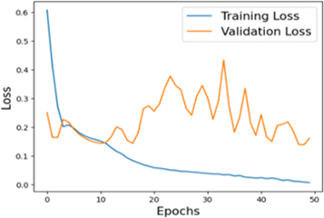
The accuracy plot in Figure 7 reveals that the training accuracy starts at approximately 82% in the initial epoch and steadily increases, achieving nearly 98% by the end of 50 epochs. Similarly, validation accuracy starts slightly lower at around 81% and reaches approximately 96%, demonstrating consistent performance and generalization across unseen data. The loss plot highlights a steady decline in training loss, starting at an initial value of about 0.6 and dropping to nearly 0.1 by the 50th epoch. Validation loss begins at approximately 0.5, with noticeable fluctuations during early epochs, stabilizing around 0.2 toward the end. This reduction in both training and validation losses, combined with the high accuracy values, confirms the robustness of the proposed method in optimizing and learning effectively while maintaining generalization to unseen data.
(a)
(b)
Figure 7. Accuracy and loss plot
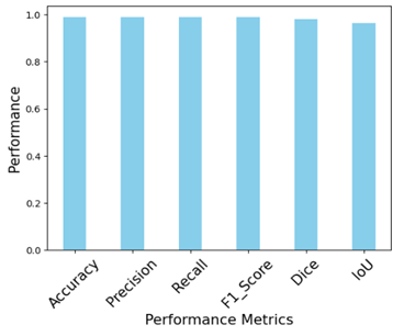
Figure 8. Performance of the proposed model
The plot in Figure 8 showcasing the performance metrics of the proposed model for accurate liver disease prediction demonstrates outstanding results across various evaluation parameters. The accuracy of 98.86% indicates that the model correctly classifies most of the liver disease cases, reflecting a strong overall performance. The precision and recall, both at 99.01%, suggest that the model not only correctly identifies positive cases (precision) but also captures almost all of the true positive cases (recall), which is crucial for medical diagnosis were missing a case can be critical. The F1-score, also at 99.01%, reflects a balanced performance between precision and recall, ensuring that the model does not favor one over the other. The Intersection over Union (IoU) of 98% indicates a high overlap between the predicted and actual regions of interest, highlighting the model's effectiveness in identifying relevant features for liver disease detection. Lastly, the Dice coefficient of 99.01% reinforces the model's reliability in accurately segmenting the liver disease area, with a strong correlation between the predicted and ground truth segments.
4.3 Comparative study
Table 2 highlights the performance of the model for liver disease prediction across different classes, with the precision, recall, F1-score, and support for each class as well as overall metrics. For class 0 (likely representing non-disease cases or the negative class), the model achieves a precision of 99%, indicating that almost all predicted negative cases are correct. The recall is also 99%, which means that the model successfully identifies 99% of the true negative cases. The F1-score of 99% indicates that the precision and recall are well balanced for this class, ensuring the model performs optimally in detecting negative cases. With 368 support, this class has a larger number of instances, and the model handles it well with these high scores. For class 1 (likely representing liver disease cases or the positive class), the model reports slightly lower but still impressive scores: precision and recall both at 98%, meaning that while the model may miss a few positive cases or make slightly more false positives compared to class 0, it still performs very well. The F1-score for class 1, which has a total of 160 instances, is obtained as 98% that show robust performance as it is effectively balancing precision and recall. The overall accuracy of model is 99% that demonstrates its strong generalization capability and the majority of both classes are accurately predicted. The macro average is also 99% for precision, recall, and F1-score is an indication of models consistency amongst the different classes because it gives an equal weight to the performance of each class. The weighted average is taken into consideration to the support for each class. The weighted average is also 99% for all metrics which is indicating that the model performs equally well across both the classes though there is variation in the number of instances. The overall performance proposes that the proposed model is highly effective and reliable for liver tumor prediction in early stage.
Table 2. Class-wise performance of the proposed model
|
|
Precision |
Recall |
F1-Score |
Support |
|
0 |
99 |
99 |
99 |
368 |
|
1 |
98 |
98 |
98 |
160 |
|
Accuracy |
99 |
99 |
99 |
528 |
|
Macro average |
99 |
99 |
99 |
528 |
|
Weighted average |
99 |
99 |
99 |
528 |
(a)
(b)
(c)
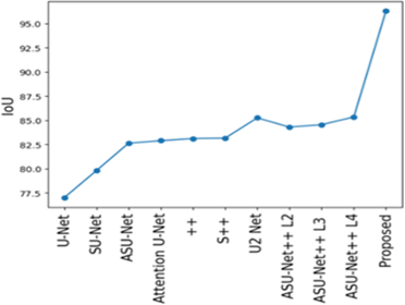
Figure 9. Comparative performance of the proposed model based on (a) MSE (b) Dice (c) IoU
The proposed method, in comparison to existing methods, show better performance in segmentation and prediction of liver tumors shown in Figure 9. The outcomes are measured particularly with the parameters as Intersection over Union (IoU), Dice coefficient and Mean Squared Error (MSE). The proposed model has higher values of IoU that reflects that it effectively capturing the true boundaries of the affected area and thus provides more precise segmentation. This is very important in medical imaging because accuracy in boundaries of affected areas directly impacts diagnosis and treatment planning. In addition to this, the MSE is very low that indicates ability of the model to generate predictions that are closer to the actual. The lower error is a measure of efficiency of model in minimizing discrepancies between predicted and actual affected areas thereby ensuring more reliable predictions. Finally, Dice coefficient is a measure of similarity between the predicted and true segmentation and for the proposed model it is significantly higher. This indicates enhanced capability of model to correctly identify and segment affected areas of liver. These results obtained through IoU, MSE and Dice clearly indicate the better performance of the proposed model over existing methods. Thus, the proposed model is a more accurate, reliable and effective solution for liver tumor prediction and segmentation adding a valuable tool in medical diagnostics.
4.4 Sensitivity analysis of anisotropic diffusion parameters
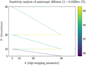
The results of the sensitivity analysis are shown in Table 3 and Figure 10. The Dice scores remained consistently high (above 97%) across a wide range of values for the parameters k, λ, and N, demonstrating the stability of the proposed processing pipeline. The best performance was observed when using moderate values for k (10 to 20) and the number of iterations N (10 to 20), with a time step λ between 0.10 and 0.15. In these settings, Dice scores exceeded 99%. When the number of iterations was too small or the time step too large, performance slightly declined due to under-smoothing (leaving residual noise) or over-smoothing (blurring important edge details). Overall, the results confirm that the model is robust to changes in these parameters and support the baseline parameter settings used in earlier sections.
Table 3. Representative sensitivity results for anisotropic diffusion filtering parameters
|
Setting |
(k, λ, N) |
Dice (%) |
IoU (%) |
MSE |
|
Baseline (used in main study) |
(20, 0.15, 10) |
99.01 ± 0.45 |
98.00 ± 0.60 |
0.0012 ± 0.0004 |
|
Best observed |
(10, 0.10, 20) |
99.25 ± 0.32 |
98.40 ± 0.42 |
0.0009 ± 0.0003 |
|
Over-smoothed (high λ, large N) |
(40, 0.25, 40) |
97.40 ± 0.90 |
95.80 ± 1.10 |
0.0035 ± 0.0010 |
|
Under-smoothed (low N) |
(5, 0.05, 5) |
95.80 ± 1.20 |
93.90 ± 1.40 |
0.0060 ± 0.0020 |
Figure 10. Heatmap showing Dice scores (%) across anisotropic diffusion parameters k and number of iterations N at λ = 0.10
4.5 Baseline classifier comparisons
To evaluate the effectiveness of the proposed WOA-SVM classifier, we compared its performance against baseline classifiers: standard SVM without optimization, Random Forest, and CNN. Table 4 summarizes the results. WOA-SVM achieved the highest accuracy (96.5%) and F1-score (95.9%), outperforming the conventional SVM (93.2%), Random Forest (91.8%), and CNN (94.5%). These results demonstrate that WOA-based optimization significantly enhances SVM performance, while maintaining lower computational complexity compared to CNN-based approaches.
Table 4. Comparison of classification performance with different classifiers
|
Classifier |
Accuracy (%) |
Precision (%) |
Recall (%) |
F1-Score (%) |
|
Random Forest (100 trees) |
91.8 |
92.0 |
91.5 |
91.7 |
|
Standard SVM (RBF kernel) |
93.2 |
93.5 |
92.8 |
93.1 |
|
CNN (3 conv layers) |
94.5 |
94.8 |
94.3 |
94.5 |
|
Proposed WOA-SVM |
96.5 |
96.2 |
95.7 |
95.9 |
4.6 Convergence comparison of optimizers
Figure 11 shows the convergence curves (validation fitness vs iteration) averaged across 5 runs for WOA, PSO, and GA. WOA demonstrates faster convergence towards lower validation fitness and smaller variance across runs compared to GA and comparable or better convergence than PSO in our setting. This supports the choice of WOA as an effective optimizer for SVM hyperparameter tuning in this application.
Figure 11. Convergence of optimizers
The proposed model is suitable for real-time clinical applications due to its low inference time and moderate model size. Its efficiency allows integration into standard hospital systems, enabling rapid and reliable decision support for clinicians.
In conclusion, the proposed method showcasing the significant advancements in both segmentation and classification for liver tumor prediction, specifically in early-stage tumor detection. Anisotropic diffusion filtering that used in the proposed method successfully reduces noise and preserves the critical structures of liver tissues so there is higher clarity in medical images. This pre-processing technique leads to the exceptional performance of proposed model. This also reflects in the segmentation results showing an IoU of 98% and a Dice coefficient of 99.01% thereby indicating a high degree of overlap between the predicted and actual regions. Prediction of liver tumor regions is précised as the Mean Squared Error (MSE) is also minimum. The presence of small and obscured tumors can be detected due to the integration of an Attention based U-TransNet which improves segmentation. Macro level features are captured through the U-Net component while the Transformer’s attention mechanism focuses on the fine details, resulting in more accurate early detection. Finally, the classification phase which is optimized with the Whale Optimization Algorithm (WOA), improves classification accuracy to 99%. It indicated that classifiers not only performance well but also handles class disparity effectively by giving higher weight to samples at early stage. This results in 99% of a precision, recall, and F1-score of the SVM classifier, confirming the robustness of model. Overall, the integration of advanced noise reduction with hybrid segmentation using attention mechanisms and metaheuristic-optimized classification leads to a complete solution for early stage liver tumor detection. A limitation of this study is the use of DeepLesion, which, although diverse, is not liver-specific. Future work will include validation on liver-focused datasets to further confirm the applicability of U-TransNet in clinical liver tumor segmentation.
[1] Zhang, H., Guo, L., Wang, D., Wang, J., et al. (2021). Multi-source transfer learning via multi-kernel support vector machine plus for B-mode ultrasound-based computer-aided diagnosis of liver cancers. IEEE Journal of Biomedical and Health Informatics, 25(10): 3874-3885. https://doi.org/10.1109/JBHI.2021.3073812
[2] Metastatic Cancer. http://www.cancer.ca/en/cancerinformation/cancer-type/metastatic-cancer/liver-metastases/?region=on.
[3] Tang, W., Zou, D., Yang, S., Shi, J., Dan, J., Song, G. (2020). A two-stage approach for automatic liver segmentation with Faster R-CNN and DeepLab. Neural Computing and Applications, 32(11): 6769-6778. https://doi.org/10.1007/s00521-019-04700-0
[4] Knipe, H. (2025). Cholangiocarcinoma. https://radiopaedia.org/articles/cholangiocarcinoma.
[5] Rajput, D., Bejoy, B.J. (2024). Optimized deep maxout for breast cancer detection: Consideration of pre-treatment and in-treatment aspect. Multimedia Tools and Applications, 83(10): 31017-31047. https://doi.org/10.1007/s11042-023-16505-4
[6] Lakshmipriya, B., Pottakkat, B., Ramkumar, G. (2023). Deep learning techniques in liver tumour diagnosis using CT and MR imaging-A systematic review. Artificial Intelligence in Medicine, 141: 102557. https://doi.org/10.1016/j.artmed.2023.102557
[7] Nainamalai, V., Prasad, P.J.R., Pelanis, E., Edwin, B., Albregtsen, F., Elle, O.J., Kumar, R.P. (2022). Evaluation of clinical applicability of automated liver parenchyma segmentation of multi-center magnetic resonance images. European Journal of Radiology Open, 9: 100448. https://doi.org/10.1016/j.ejro.2022.100448
[8] Prakash, N.N., Rajesh, V., Namakhwa, D.L., Pande, S.D., Ahammad, S.H. (2023). A DenseNet CNN-based liver lesion prediction and classification for future medical diagnosis. Scientific African, 20: e01629. https://doi.org/10.1016/j.sciaf.2023.e01629
[9] Balasubramanian, P.K., Lai, W.C., Seng, G.H., C, K., Selvaraj, J. (2023). Apestnet with mask r-CNN for liver tumor segmentation and classification. Cancers, 15(2): 330. https://doi.org/10.3390/cancers15020330
[10] Kierner, S., Kucharski, J., Kierner, Z. (2023). Taxonomy of hybrid architectures involving rule-based reasoning and machine learning in clinical decision systems: A scoping review. Journal of Biomedical Informatics, 144: 104428. https://doi.org/10.1016/j.jbi.2023.104428
[11] Munoz-Gama, J., Martin, N., Fernandez-Llatas, C., Johnson, O.A., et al. (2022). Process mining for healthcare: Characteristics and challenges. Journal of Biomedical Informatics, 127: 103994. https://doi.org/10.1016/j.jbi.2022.103994
[12] Ma, J., Deng, Y., Ma, Z., Mao, K., Chen, Y. (2021). A liver segmentation method based on the fusion of VNet and WGAN. Computational and Mathematical Methods in Medicine, 2021(1): 5536903. https://doi.org/10.1155/2021/5536903
[13] Rahman, H., Bukht, T.F.N., Imran, A., Tariq, J., Tu, S., Alzahrani, A. (2022). A deep learning approach for liver and tumor segmentation in CT images using ResUNet. Bioengineering, 9(8): 368. https://doi.org/10.3390/bioengineering9080368
[14] Liu, Z., Song, Y.Q., Sheng, V.S., Wang, L., Jiang, R., Zhang, X., Yuan, D. (2019). Liver CT sequence segmentation based with improved U-Net and graph cut. Expert Systems with Applications, 126: 54-63. https://doi.org/10.1016/j.eswa.2019.01.055
[15] Fang, X., Xu, S., Wood, B.J., Yan, P. (2020). Deep learning-based liver segmentation for fusion-guided intervention. International Journal of Computer Assisted Radiology and Surgery, 15(6): 963-972. https://doi.org/10.1007/s11548-020-02147-6
[16] Almotairi, S., Kareem, G., Aouf, M., Almutairi, B., Salem, M.A.M. (2020). Liver tumor segmentation in CT scans using modified SegNet. Sensors, 20(5): 1516. https://doi.org/10.3390/s20051516
[17] Di, S., Zhao, Y., Liao, M., Yang, Z., Zeng, Y. (2022). Automatic liver tumor segmentation from CT images using hierarchical iterative superpixels and local statistical features. Expert Systems with Applications, 203: 117347. https://doi.org/10.1016/j.eswa.2022.117347
[18] Deshmukh, P.V., Shahade, A.K., Shahade, M.R., Wankhede, D.S., Gohatre, P.H. (2025). Breast cancer detection using a novel hybrid machine learning approach. Ingenierie des Systemes d'Information, 30(3): 565-567. https://doi.org/10.18280/isi.300301
[19] Zhou, Y., Kong, Q., Zhu, Y., Su, Z. (2023). MCFA-UNet: Multiscale cascaded feature attention U-Net for liver segmentation. IRBM, 44(4): 100789. https://doi.org/10.1016/j.irbm.2023.100789
[20] Sun, C., Xu, A., Liu, D., Xiong, Z., Zhao, F., Ding, W. (2019). Deep learning-based classification of liver cancer histopathology images using only global labels. IEEE Journal of Biomedical and Health Informatics, 24(6): 1643-1651. https://doi.org/10.1109/JBHI.2019.2949837
[21] Trivizakis, E., Manikis, G.C., Nikiforaki, K., Drevelegas, K., Constantinides, M., Drevelegas, A., Marias, K. (2018). Extending 2-D convolutional neural networks to 3-D for advancing deep learning cancer classification with application to MRI liver tumor differentiation. IEEE Journal of Biomedical and Health Informatics, 23(3): 923-930. https://doi.org/10.1109/JBHI.2018.2886276
[22] Reddy, N.N., Ramkumar, G. (2023). Liver segmentation and classification in computed tomography images using convolutional neural network and comparison of accuracy with support vector machine. AIP Conference Proceedings, 2821(1): 050023. https://doi.org/10.1063/5.0158596
[23] Dickson, J., Linsely, A., Nineta, R.A. (2023). An integrated 3D-sparse deep belief network with enriched seagull optimization algorithm for liver segmentation. Multimedia Systems, 29(3): 1315-1334. https://doi.org/10.1007/s00530-023-01056-3
[24] Perona, P., Malik, J. (2002). Scale-space and edge detection using anisotropic diffusion. IEEE Transactions on Pattern Analysis and Machine Intelligence, 12(7): 629-639. https://doi.org/10.1109/34.56205
[25] Garg, A., Bajaj, A., Lal, R. (2020). Brain tumor detection using image processing based on anisotropic filtration techniques. In Micro-Electronics and Telecommunication Engineering: Proceedings of 3rd ICMETE 2019, pp. 365-373. https://doi.org/10.1007/978-981-15-2329-8_37