Marwa Arabi![]() | Youcef Zennir
| Youcef Zennir![]() | Hichem Bounezour
| Hichem Bounezour![]() | Mohamed Benghanem*
| Mohamed Benghanem*![]() | J.E.S. Garcia
| J.E.S. Garcia![]() | M. Wadi
| M. Wadi![]()
© 2025 The authors. This article is published by IIETA and is licensed under the CC BY 4.0 license (http://creativecommons.org/licenses/by/4.0/).
OPEN ACCESS
Wind turbines operate under highly dynamic conditions influenced by unpredictable wind profiles and external disturbances. The nonlinear characteristics of their dynamic models further complicate their modeling and control. This research focuses on optimizing the power output of a Wind Energy Conversion System (WECS) equipped with a Permanent Magnet Synchronous Generator (PMSG). To achieve this, a Maximum Power Point Tracking (MPPT) strategy is developed, integrating an innovative nonlinear PI controller. The parameters of this controller are fine-tuned using advanced meta-heuristic optimization techniques, including Particle Swarm Optimization (PSO), Harris Hawks Optimization (HHO), and Golden Jackal Optimization (GJO). Simulation results highlight the superior performance of the GJO-NLPI controller, demonstrating exceptional accuracy and rapid response in regulating mechanical rotation speed, while effectively reducing overshoot. The proposed control architecture showcases significant advancements in power extraction efficiency and dynamic performance.
Wind Energy Conversion System (WECS), Permanent Magnet Synchronous Generator (PMSG), Maximum Power Point Tracking (MPPT), architecture, nonlinear PI controller, PSO algorithm, HHO algorithm, GJO algorithm
In various industrial and residential sectors. This constant rise has accentuated the pressure on traditional energy resources, particularly oil and gas, leading to growing concerns about their high cost, rapid depletion, and negative environmental impacts, particularly the emissions of greenhouse gases that lead to climate change [1, 2]. Faced with these challenges, renewable energies have emerged as a viable and sustainable alternative. They not only offer a response to the growing energy demand but also contribute to mitigating the environmental impacts associated with electricity production [3]. Out of the different sustainable power sources; wind energy has captured particular attention due to its abundant availability and capacity for rapid development. Moreover, technological advances in the have significantly increased wind turbine systems' profitability and efficiency [4-6]. In order to transform wind energy into electrical power, the Wind Energy Conversion System (WECS) uses a wind turbine in conjunction with an electric generator. This conversion can be direct or through a gearbox, followed by an electronic power interface that ensures the connection of the generator either to autonomous loads or to the electrical grid [6]. Wind turbines are designed to operate at either a fixed speed (FSWT) or a variable speed (VSWT), depending on wind characteristics [7, 8]. FSWTs, although simple, have limitations such as a restricted operating range and high mechanical constraints requiring complex gearboxes [7]. In contrast, VSWTs are designed to optimize energy production by adjusting their rotational speed to match wind speed, thus minimizing losses and power fluctuations [9-12]. A significant challenge in maximizing the efficiency of VSWTs lies in enhancing power efficiency throughout a wide range of wind velocities. This requires the employment of Maximum Power Point Tracking (MPPT) techniques. Notable among them are the Tip Speed Ratio (TSR) algorithm [13, 14], Power Signal Feedback (PSF) [13-15], Optimal Torque (OT) algorithms [16, 17], Hill Climb Search (HCS) MPPT algorithms, Incremental Conductance (INC), Optimal Relationship-Based (ORB) and other traditional techniques have demonstrated their effectiveness in enhancing wind turbine performance [13, 17]. Several scientific studies have been conducted to optimize MPPT results by proposing various advanced control strategies [18]. Kaoutar et al. [19] introduced a hybrid MPPT control combining P&O (Perturb and Observe) controllers with a neural network, demonstrating good precision but exhibiting high overshoot and slow response times. Similarly, Salma et al. [20] developed an optimal hybridization between Proportional-Integral (PI) control and advanced sliding mode control based on Particle Swarm Optimization (PSO) that unfortunately resulted in a very long response time. Moreover, fuzzy optimization strategies for MPPT control architectures have been explored by Belkacem et al. [21], who reported high overshoot; Mohammad et al. [22] proposed a hybridization of fuzzy and sliding mode controllers, which faced issues with chattering and overshoot. Finally, Benkada et al. [23] Investigated MPPT control for wind power system conversion using a T-S (Takagi-Sugeno) fuzzy approach revealing a considerable error margin. Despite these advancements, the classic PID controller remains predominant in the industry due to its reliability and simplicity of implementation. On the other hand, its sensitivity to nonlinear dynamics is well-known. To overcome this limitation, new nonlinear PID controllers have been developed and successfully applied to complex systems such as the Antenna Azimuth Position System [24, 25], robotic systems [26], and continuous stirred tank reactors [27], thereby offering significantly improved performance [28]. An approach to introducing nonlinearity into the PID controller involves using nonlinear gains, which can be achieved through hyperbolic functions [26, 29-31] and other nonlinear functions such as exponentials or sigmoid functions [25, 32, 33]. Furthermore, Al-Samarraie and Abbas [33] proposed a method to make the integral term nonlinear by incorporating an arctangent function, thereby enhancing the controller's robustness against varying disturbances. In the context of wind energy systems, several studies have assessed the potential of nonlinear PI (NLPI) controllers. Hazzab et al. [34]. demonstrated their effectiveness in wind turbine emulators, reporting improved robustness and reduced overshoot compared with conventional PI controllers. Ren et al. [35] highlighted their application to variable pitch control, noting enhanced performance but also challenges in maintaining stability under rapidly fluctuating wind conditions. Liu et al. [36] investigated nonlinear PI/PD pitch controllers, which improved power regulation but required meticulous gain scheduling and introduced additional implementation complexity. Overall, these studies confirm the capability of NLPI controllers to improve system performance, while also highlighting their main limitation: strong dependence on empirically tuned parameters, often lacking systematic adaptation or optimization, which can significantly affect performance. Charrak's review [37] on computational intelligence applications in stability analysis underscores how advanced optimization techniques can mitigate such limitations in nonlinear systems, particularly under dynamic operating conditions. Building on these findings, the present work proposes a novel NLPI controller design that integrates the aforementioned approaches to enhance robustness. Specifically, hyperbolic gains are employed for self-tuning, while arctangent terms are incorporated into the integral component to improve resilience against variable wind disturbances. To address the difficulty of manual parameter tuning, optimization is carried out using well-regarded algorithms such as Particle Swarm Optimization (PSO) and Harris Hawks Optimization (HHO), both recognized for their effectiveness in determining PI controller gains [38-39]. Recent work [40-41] further validates PSO's capability in complex nonlinear systems, successfully estimating parameters for chaotic dynamics like the Chua circuit—a testament to its adaptability for wind turbine control challenges. Furthermore, the recently introduced Golden Jackal Optimization (GJO) algorithm [42], inspired by the hunting patterns of golden jackals, is also applied. The proposed method aims to deliver improved accuracy, robustness, and dynamic performance under varying wind profiles. The key contributions of this study are summarized as follows:
1. The novel Nonlinear PI (NLPI) controller developed in this study optimizes wind turbine speed control, enabling more efficient power extraction from varying wind profiles.
2. By integrating advanced metaheuristic algorithms (PSO, HHO, GJO) with the NLPI controller, the study achieves superior system performance in terms of accuracy, robustness, and response time. The study demonstrates the robustness of the NLPI controller under variable and step wind speed profiles, ensuring reliable operation under real-world conditions. The innovative integration of an arctangent function into the controller significantly minimizes static error (3.15e-6) and improves response time (0.0322 seconds), outperforming conventional PI controllers. The research provides valuable insights into the effectiveness of different metaheuristic optimization methods, highlighting the superior performance of the GJO algorithm in enhancing wind turbine system control. A detailed mathematical model developed using MATLAB/Simulink validates the proposed methods, offering a reliable platform for further advancements in wind turbine technology. The advanced NLPI controller and its optimization strategies could be applied to other renewable energy systems, enhancing control performance across diverse applications. The study lays the groundwork for integrating the optimized wind turbine model into a broader energy conversion system, paving the way for comprehensive renewable energy solutions. The remainder of this work is organized as follows: Section 2 covers the modeling of the wind turbine system, Section 3 presents the wind speed control architecture, and Section 4 discusses the three WECS optimization algorithms PSO, HHO, and GJO. The simulation results are presented in Section 5. Finally, Section 6 provides the conclusions and perspectives for future research.
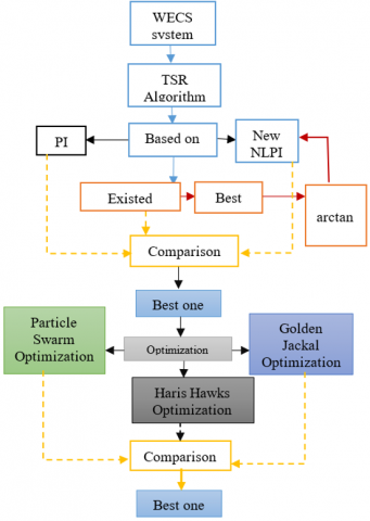
The methodology of our study is illustrated in the following figure (Figure 1):
Figure 1. Methodology of this study
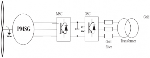
The grid-connected global Wind Energy Conversion System is depicted in Figure 2. The subsequent section provides a detailed model of the wind turbine and the Permanent Magnet Synchronous Generator (PMSG).
Figure 2. Schematic representation of a standard grid-integrated WECS
2.1 Wind turbine modeling
The mechanical power extracted by the wind turbine $P_{{turb }}$ (KW) can be mathematically represented, as detailed in the following Eq. (1) [43]:
$P_{ {turb }}=0.5 C_p(\lambda, \beta) \rho \pi R^2 V^3$ (1)
where, ρ represents air density, V denotes wind velocity (in m/s), R symbolizes the wind turbine blades diameter (in m), and $C_p$ (λ, β) represents the power coefficient of wind turbines, that describes an approximation to empirical data of a wind turbine, as defined in Eq. (2):
$C_p=\left[0.5176\left(\frac{116}{\lambda^{\prime}}\right)-0.4 \beta-5\right] exp \left(\frac{-21}{\lambda^{\prime}}\right)+0.0068 \lambda$ (2)
With:
$\lambda^{\prime}=\frac{1}{\lambda+0.08 \beta}-\frac{0.035}{\beta^3+1}$ (3)
$\lambda=\frac{w_{ {turb }} R}{V}$ (4)
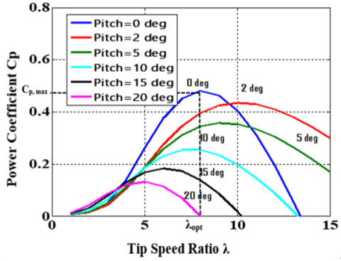
Here, λ represents the tip-speed-ratio, β is the blade pitch angle, and $w_{ {turb }}$ denotes the mechanical speed of the turbine blades (in rad/s). Figure 3 shows the features of the turbine that was used.
Figure 3. Variation of the aerodynamic power coefficient Cp as a function of the tip speed ratio λ and the pitch angle β
The wind turbine's mechanical torque $T_{ {turb }}$ (N.m-1) is obtained using Eq. (5) as follows.
$T_{ {turb }}=\frac{P_{ {turb }}}{w_{ {turb }}}=\frac{0.5 C_p(\lambda, \beta) \rho \pi R^2 V^3}{w_{ {turb }}}$ (5)
The gearbox is necessary to adjust the wind turbine's rotor speed and torque to be compatible with the PMSG, as described by the following equation:
$\left\{\begin{array}{l}w_m=G . w_{ {turb }} \\ T_m=\frac{1}{G} . T_{{turb }}\end{array}\right.$ (6)
where, $w_m$ is the PMSG's mechanical rotating speed, G is the gear ratio coefficient, and $T_m$ is the wind torque imparted to the generator rotor.
The representation of mechanical transmission is demonstrated by the following Eq. (7):
$j \frac{d w_m}{d t}=T_m-T_{e m}-\frac{f}{j} w_m$ (7)
where, f signifies friction, j represents inertia, and $T_{e m}$ is electromagnetic torque.
2.2 Permanent magnets synchronous generator
According to Eq. (8), the PMSG generates an electromagnetic torque [40].
$T_{e m}=\frac{3 P}{2}\left(\lambda_r i_{q s}-\left(L_d-L_q\right) i_{d s} i_{q s}\right)$ (8)
The synchronous generator's dq-axis self-inductance is represented by $L_d$ (H) and $L_q$ (H), P is the number of pole pairs and $\lambda_r$ (wb(rms)) is the rotor flux linkages, the stator current along the PMSG generator's dq-axis is represented by $i_{d s}$ and $i_{q s}$ as shown in Eq. (9):
$\left\{\begin{array}{c}\frac{d i_{d s}}{d t}=-\frac{R_s}{L_d} i_{d s}+\frac{L_q}{L_d} w g i_{q s}-\frac{1}{L_d} v_{d s} \\ \frac{d i_{q s}}{d t}=-\frac{R_s}{L_q} i_{q s}+\frac{L_d}{L_q} w_g i_{d s}-\frac{1}{L_q} w_g \lambda_r-\frac{1}{L_q} v_{q s}\end{array}\right.$ (9)
where, $w_g$ is the generator's mechanical rotor speed, which can be obtained from $w_m$ in the manner described below:
$w_g=P * w_m$ (10)
$R_s$: indicates the resistance of the stator winding in the PMSG generator.
$v_{q s}$ and $v_{d s}$: refer, respectively, to the stator voltages along the quadrature and direct axes.
The following equation provides the modeling of these voltage components:
$\left\{\begin{array}{c}v_{d s}=-R_s i_{d s}+L_q w_g i_{q s}-L_d \frac{d i_{d s}}{d t} \\ v_{q s}=-R_s i_{q s}-L_d w_g i_{d s}+w_g \lambda_r-L_q \frac{d i_{q s}}{d t}\end{array}\right.$ (11)
3.1 Maximum Power Point Tracking
Algorithm's outstanding effectiveness and fast responsiveness make it one of the most popular MPPT techniques. By modifying the generator's rotating speed, the TSR control approach increases power extraction while preserving the TSR at an ideal value that can be determined empirically [13, 18, 44-47]. Both wind and generator speed measurements are necessary for the algorithm to obtain the best TSR ($\lambda_{o p t}$) and extract the most power. Eq. (12) is used to calculate the ideal rotational speed in the following manner:
$w_{ {m.opt }}=\frac{\lambda_{ {opt }} V}{R}$ (12)
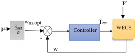
The block diagram in Figure 4 provides a clear depiction of a WECS employing TSR control. The ideal rotational speed and the real rotational speed are continuously compared, and any differences are fed into a controller. To reduce this discrepancy, the controller then modifies the generator's speed. As a result, the method guarantees that the mechanical power output of the generator is in close agreement with the highest possible mechanical power [46].
Figure 4. TSR MPPT algorithm of WECS
3.2 Controllers design
Classical PI controllers are extensively used in industry because of their straightforward architecture, adaptability, and accurate control capabilities. These controllers rely on two primary parameters: the proportional gain ($k_p$) and the integral gain ($k_i$), which play pivotal roles in shaping system performance and require careful selection. The control law of a linear PI controller is defined in Eq. (13):
$U(t)=k_p e(t)+k_i$ (13)
However, linear PI controllers face significant challenges when dealing with changes or uncertainties in operational conditions and nonlinear system dynamics. Specifically, they suffer from balancing rapid response and minimal overshoot. High gains can effectively correct large errors but may introduce unwanted overshooting and oscillations. In contrast, low gains stabilize the system but result in slower response times. A dynamic approach to gain adjustment is essential to overcome these challenges: higher gains (aggressive) are appropriate for addressing significant errors, while lower gains (conservative) are preferable for minor errors. Recognizing these limitations, nonlinear PI controllers have become a viable substitute for improving the performance of systems with nonlinear dynamics [31]. The control low of the nonlinear PI controller will be as represented in Eq. (14):
$U_{N L}(t)=\overline{\left(k_p\right)} e(t)+\overline{\left(k_l\right)} \int e(t) d t$ (14)
where, $\overline{\left(k_p\right)}$ and $\overline{\left(k_{\imath}\right)}$ represent the NLPI controller's self-adjusting nonlinear gains.
Various researchers have explored these, using different mathematical functions to improve the performance of control systems. Thus:
Shi et al. [25] proposed nonlinear gains based on the hyperbolic function "sech" as indicated in Eq. (15):
$U_{ {sech }}(t)=\left(k_{p 1}\left(1-\operatorname{sech}\left(k_{p 2} e(t)\right)\right)+k_{p 0}\right) e(t)+k_{i 1} \operatorname{sech}\left(k_{i 2} e(t)\right) \int e(t) d t$ (15)
where,
$\operatorname{Sech}(x)=\frac{2}{e^x+e^{-x}}$ (16)
Another hyperbolic function based on the "cosh" function was proposed by Ruderman et al. [29], as shown by Eq. (17):
$U_{cosh }(t)=2 \cosh \left(\alpha_1 e(t)\left(k_{p 0} e(t)+k_{i 0} \int e(t) d t\right)\right)$ (17)
where,
$\cosh x=\frac{e^x+e^{-x}}{2}$ (18)
Xu [32] and Tian [24] proposed the use of exponential functions as shown in Eqs. (19) and (20), respectively:
$U_{e x p_{X u}}(t)=\left(\frac{k_{p 1}}{1+k_{p 2} e^{\alpha_1 {sign}(e(t))}+k_{p 0}}\right) e(t)+\left(\frac{k_{i 1}}{1+k_{i 2} e^{\alpha_2 {sign}(e(t))}+k_{i 0}}\right) \int e(t) d t$ (19)
$U_{exp _{ {Tian }}}(t)=\left(k_{p 0}-\left(k_{p 0}-k_{p 1}\right)\left(1+k_{p 2}|e(t)|\right) e^{\left(-k_{p 2}|e(t)|\right)} e(t)+\left(k_{i 0}-\left(k_{i 0}-k_{i 1}\right)\left(1+k_{i 2}|e(t)|\right) e^{\left(-k_{i 2}|e(t)|\right)} \int e(t) d t\right)\right.$ (20)
Seraji proposed using sigmoid functions to dynamically alter the controller gains in accordance with errors, with his formulations detailed in the equations referenced [30]:
$U_{ {sigmiod }}(t)=\left(k_{p 1}\left(\frac{2}{1+e^{-k_{p 2} e(t)}-1}-1\right)+k_{p 0}\right) e(t)+\left(k_{i 1}\left(\frac{2}{1+e^{-k_{i 2} e(t)}-1}-1\right)+k_{i 0}\right) \int e(t) d t$ (21)
With: Constants Kp0, Kp1, Kp2, Ki0, Ki1, Ki2, α1, α2, and α3, modify the range and the rate of variation for the nonlinear PI controller.
Simulation results presented in Section 5 of integrating the NLPI mentioned above controllers demonstrated the superior efficiency of the controller proposed by Shi et al. To further enhance its performance against variable disturbances, an integral based on the arctangent function of the error is employed instead of the error itself. This improvement aims to increase the controller's ability to attenuate the effects of variable disturbances on system dynamics. Through a nonlinear approach, integral control accumulates error differently: instead of simply integrating the error, the arctangent function of the error is employed. This allows for better adaptation to disturbance variations and reduces the effects of limit cycles, where the system enters a loop of bounded oscillation. This method also adjusts the integral gain based on how close the system state is to equilibrium, thereby minimizing the risk of control saturation during significant deviations from equilibrium. The novel NLPI control law is formulated as follows [34]:
$U_{ {novel }\, N L}(t)=\left(k_{p 1}\left(1-\operatorname{sech}\left(k_{p 2} e(t)\right)\right)+k_{p 0}\right) e(t)+k_{i 1} \operatorname{sech}\left(k_{i 2} e(t)\right) \int \tan ^{-1}\left(\alpha_3 \mathrm{e}(\mathrm{t})\right) d t$ (22)
where, $\alpha_3$ is a design parameter.
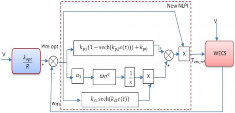
Figure 5 displays the NLPI controller's integration into the wind turbine's MPPT control architecture.
Figure 5. TSR MPPT algorithm based Novell NLPI of WECS
Nature-inspired metaheuristic algorithms are considered to be the most effective methods for addressing intricate optimization challenges. In this study, we are utilizing a minimization fitness function that is the integral of the absolute error (IAE) and is given as Eq. (23):
$I A E=\int|e(t)| d t$ (23)
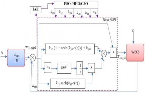
The primary purpose of this fitness function is to examine the efficacy of the optimization algorithms, as it tells us the difference between the desired and actual outputs. Our target with the diminution of the IAE is to increase both the accuracy and efficiency of the control system in different scenarios, thereby ensuring a more substantial and stable operating point. Several simulated runs of different fitness functions contribute to each algorithm to calculate the optimal parameters of a newly designed nonlinear PI controller. This approach ensures that the controller is meticulously tuned to enhance system performance, tailored to the specific dynamics of the system. Figure 6 illustrates the optimization process employed in this study, where the Particle Swarm Optimization (PSO), Harris Hawks Optimization (HHO), and Golden Jackal Optimization (GJO) algorithms are used to fine-tune the controller.
Figure 6. Metaheuristic algorithm implementation for maximum performance in the TSR MPPT control loop-based NLPI of the WECS
4.1 Particle swarm optimization algorithm
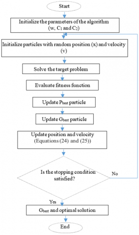
Particle Swarm Optimization (PSO) is a computational approach that falls under the category of swarm intelligence approaches and is inspired by phenomena of nature. PSO, which was first presented by Kennedy and Eberhart in 1995 [48], mimics the collective behavior of swarming organisms, such fish or birds, as they move toward a target. The method finds the optimal solution, often referred to as the global best, by moving across the search space using a collection of particles that each represent a possible solution. Particles constantly adjust their positions throughout this process by taking into account both the aggregate best position of the swarm and their individual best locations. As a result, the placements of the particles, which in this case reflect the PI gains, are iteratively improved using well-defined mathematical Eqs. (24) and (25).
$V_{i,}^{t+1}=w V_i^t+c_1 R_{1 i}^t\left(p_{i, { best }}^t-x_i^t\right)+c_2 R_{2 i}^t\left(G_{ {best }}^t-X_i^t\right)$ (24)
$X_{i,}^{t+1}=w V_{i,}^{t+1}+X_{i, j}^t$ (25)
where, $V_{i,}^{t+1}$ and Vit denote the velocity of each particle at the current and previous iteration, respectively, $X_{i,}^{t+1}$ and $x_i^t$ represent the position of particles in the current and previous iterations, respectively, $p_{i, { best }}^t$, and $G_{b e s t}^t$ represent the personal and global best of each candidate and the hole swarm, and $c_{1,2}$ and w are the personal and global learning coefficient, inertia weight and R1,2 a random number. Figure 7 depicts the method's flowchart.
Figure 7. PSO algorithm flowchart
4.2 Haris hawks optimization algorithm
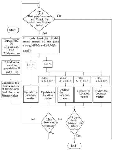
Creation of the Harris Hawks Optimization (HHO) algorithm. Three main stages comprise the framework of this population-based algorithm: exploration, the transition from exploration to exploitation, and exploitation [49, 50]. The algorithm's initial step follows the search pattern of Harris's hawks as they pursue their prey. This stage of investigation is crucial for creating a preliminary database of potential prey locations that spans a large search space. In Eq. (26), the mathematical model for this phase is explained as follows:
$x(\tau+1)=\left\{\begin{array}{c}x_r(\tau)-r_1\left|x_r(\tau)-2 r_2 x(\tau)\right| \text { for } k \geq 0.5 \\ \left(x_p(\tau)-x_m(\tau)\right) \\ -r_3\left(L_B+r_4\left(u_B-L_B\right)\right) \text { for } k<0.5\end{array}\right.$ (26)
Figure 8. Flowchart HHO algorithm
As the algorithm progresses, it shifts from exploration to exploitation. This shift happens when the hawks concentrate on identified prey. The prey's energy, denoted as E0, fluctuates between -1 and 1, reflecting the prey's attempts to evade its predators. The algorithm then enters the exploitation phase, where the hawks attack and capture prey. This phase intensively optimizes solutions by focusing on the best discoveries. The cooperative behavior of the hawks is modeled to maximize capture chances, continually adjusting solution positions to converge towards optimal solutions. The flowchart that illustrates the HHO algorithm is shown in Figure 8.
4.3 Golden Jackal Optimization
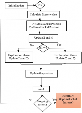
GJO is considered a biological optimization algorithm inspired and modeled after the behavior of golden jackals. These predators first discover their prey, then besiege, stimulate, and finally attack them. The following is the formulation of the mathematical framework describing this behavior [42]:
4.3.1 Search model
Initially as Eq. (27) illustrates, the prey's random location is represented in a matrix:
$\left[\begin{array}{ccccc} \quad & \Upsilon_{1,1} \Upsilon_{1, j} &\quad& \cdots & \Upsilon_{1, n} \\ \vdots & & \vdots & \ddots & \vdots \\ \quad &\Upsilon_{N, 1} \Upsilon_{N, j} & \quad &\cdots & \Upsilon_{N, n}\end{array}\right]$ (27)
The number of dimensions is denoted by n, and the total number of prey populations by N.
4.3.2 Exploration stage
Golden jackals have a strong ability to track their prey; however, capturing them is not always easy. Therefore, they often wait for another opportunity to hunt. This hunting behavior can be defined as follows (|E|>1):
$\Upsilon_1(t)=\Upsilon_M(t)-E . \mid \Upsilon_M(t)-rl.Prey(t) \mid$ (28)
$\Upsilon_2(t)=\Upsilon_{F M}(t)-E .\left|\Upsilon_{F M}(t)-{rl.Prey}(t)\right|$ (29)
Here, t represents the current iteration of the algorithm, $\Upsilon_M(t)$ and $\Upsilon_{F M}(t)$ identify the positions of the male and female jackals, Prey(t) represents the hunting position vector, and $\Upsilon_1(t)$ and $\Upsilon_2(t)$ determine the updated jackal locations.
Eq. (30) is used to determine the prey's escape energy (E):
$E=E_1 . E_0$ (30)
where:
$E_0=2 . r-1$ (31)
And
$E_1=c 1 .\left(1-\frac{t}{T}\right)$ (32)
E0 is a randomly generated value ranging from -1 to 1, T is the maximum number of repeats, c1 is a 1.5 constant, and E1 represents the decrease that occurs in the prey's energy. In Eqs. (27) and (28) $\mid \Upsilon_M(t)- rl.Prey (t) \mid$ is the distance that lies from the jackal to its prey, where rl is a series of random values depending on the Le'vy flight function (LF):
$r l=5 . \frac{L F(y)}{100}$ (33)
$L F(y)=\mu . \frac{\sigma}{100 .\left|v^{\left(\frac{1}{m}\right)}\right|}$ (34)
$\sigma=\left\{\frac{\Gamma(m+1) . \sin \left(\frac{\pi m}{2}\right)}{\Gamma\left(\frac{m+1}{2}\right) . m\left(2^{m-1}\right)}\right\}^{\frac{1}{m}}$ (35)
Here, v takes values randomly within the interval (0, 1); m is a fixed value of 1.5.
$\Upsilon(t+1)=\frac{\Upsilon_1(t)-\Upsilon_2(t)}{2}$ (36)
$\Upsilon(t+1)$ reflects the prey's current location relative to the jackals.
4.3.3 Exploitation (Besieging and Swallowing Prey)
Golden jackals persistently harass their prey in order to reduce their escape energy. This siege and consumption behavior is modeled as follows (|E|≤1):
$\Upsilon_1(t)=\Upsilon_M(t)-E .\left|\Upsilon_M(t)-\operatorname{Prey}(t)\right|$ (37)
$\Upsilon_2(t)=\Upsilon_{F M}(t)-E .\left|Y_{F M}(t)-{Prey}(t)\right|$ (38)
4.3.4 Transition from exploration stage to exploitation and convergence
The GJO algorithm transitions from exploration to exploitation by tracking the prey's energy, which decreases as it escapes. Initial energy (E0) varies randomly between -1 and 1. A decrease from 0 to -1 indicates danger for the prey, while an increase from 0 to 1 indicates boosted ability. When |E| > 1, jackals explore the search space; when |E| < 1, they exploit the prey. The search starts with selected solutions, estimating the prey's location using jackal pairs. The algorithm alternates between exploration and exploitation as E1 decreases from 1.5 to 0. The GJO algorithm concludes upon meeting convergence conditions. The GJO flowchart is displayed in Figure 9.
Figure 9. Flowchart of GJO algorithm
The simulation results of the wind turbine are obtained using the parameters listed in Table 1 [51]. All simulations were performed in MATLAB/Simulink with the solver ode45 and a relative tolerance of 1e-3. A variable-step configuration was adopted, as the model is continuous-time, with the solver automatically adjusting the integration step;
Table 1. System parameters
|
Wind Turbine |
PMSG |
||
|
Parameters |
Values |
Parameters |
Values |
|
Wind Turbine Rotor blades (R) |
2 (m) |
Rated power (Popt) |
10 KW |
|
Air density (ρ) |
1.225 |
Stator resistance (Rs) |
0.00829 Ω |
|
Pitch angle (β) |
0 |
Stator direct inductance (Ld) |
0.174 mH |
|
Optimal Tip speed ratio (λopt) |
8.1 |
Stator quadrature inductance (Lq) |
0.174 mH |
|
Maximum power coefficient $\left(c_{p_{max }}\right)$ |
0.48 |
Permanent magnet flux ($\lambda_r$) |
0.071 wb |
|
Number of pole pairs (P) |
6 |
||
|
Inertia (j) |
0.089 kg/m2 |
||
|
Friction (f) |
0.005 Nm |
||
The results of this study are presented in detail as follows.
5.1 Simulation 1: Comparison between different NLPI controllers
This simulation section compares the five previously mentioned NLPI controllers with the classic PI controller under constant and uncertain wind profiles. The parameters for all controllers were determined using the empirical trial and error method, and the optimal response was selected based on the lowest ultimate angular speed. Different Parameters Used for Each Controller are presented in Table 2.
Table 2. Different parameters used for each controller
|
Controller |
Kp0 |
Kp1 |
Kp2 |
Ki0 |
Ki1 |
Ki2 |
α1 |
α2 |
α3 |
|
PI |
2000 |
/ |
/ |
500 |
/ |
/ |
/ |
/ |
/ |
|
NLPI1 (Eq 14) |
175 |
0.98 |
5 |
/ |
100 |
0.98 |
/ |
/ |
/ |
|
NLPI2 (Eq 16) |
75 |
/ |
/ |
8 |
/ |
/ |
0.01 |
/ |
/ |
|
NLPI3 (Eq 18) |
50 |
5 |
3 |
6 |
5 |
2 |
0.98 |
0.98 |
/ |
|
NLPI4 (Eq 19) |
1500 |
500 |
0.9 |
400 |
100 |
0.9 |
/ |
/ |
/ |
|
NLPI5 (Eq 20) |
100 |
50 |
0.98 |
80 |
10 |
10 |
/ |
/ |
/ |
5.1.1 Step wind profile results
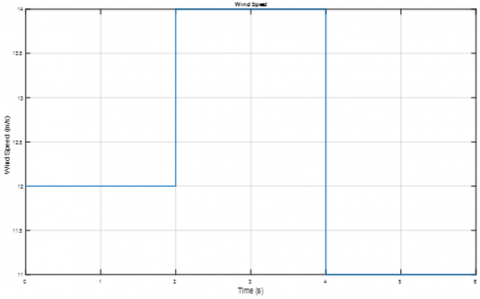
The variable wind speed acting on the turbine blades is considered a disturbance. Various operating conditions (wind speeds) are proposed to evaluate the resilience and performance of the NLPI controllers. Initially, a step wind profile ranging from 11 m/s to 14 m/s is applied, as shown in Figure 10, while the corresponding rotor speed is illustrated in Figure 11.
Figure 10. The step wind curve
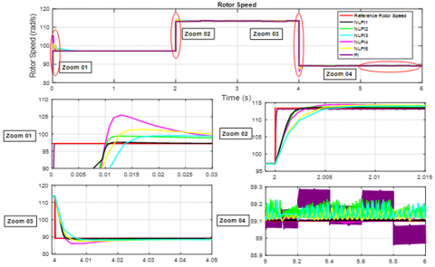
Figure 11. The curve of rotor speed with NLPI controllers under step wind profile
5.1.2 Variable wind profile results
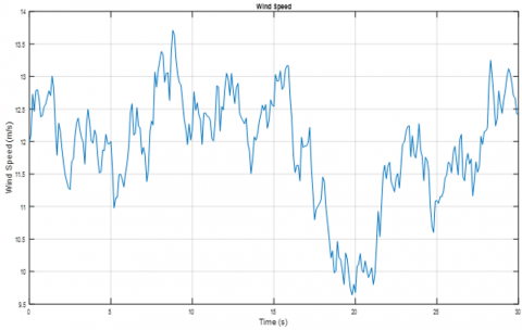
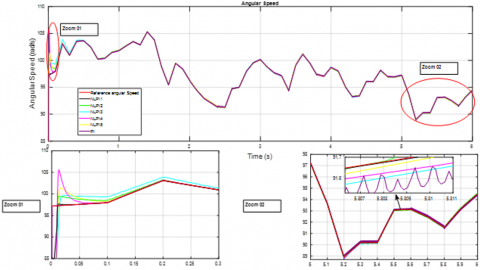
The uncertain wind profile and the corresponding rotor speed are displayed in the following Figures.
A comparison study between the results obtained with different NLPI controllers under step and variable wind profiles is presented in the table below.
As shown in Table 3, Figures 11, 12 and 13, the NLPI controllers demonstrate significantly higher efficiency and robustness than the classic PI controller in terms of error, overshoot, and response time. Among the six NLPI controllers tested, the NLPI1 controller stands out with markedly better results, exhibiting an error of 0.0007994, a response time of 0.075, and an overshoot of 0.36. This controller offers superior performance across all evaluated aspects. An arctangent term to the integral function of the error is proposed to improve this controller further. The following part presents and analyzes the optimization's outcomes.
Figure 12. The uncertain wind curve
Figure 13. The rotor speed with NLPI controllers under variable wind profile
Table 3. Comparison of results obtained with different NLPI controllers
|
Controller |
Error |
Response Time (s) |
Overshoot (rad/s) |
|
NLPI1 |
0.0007994 |
0.075 |
0.36 |
|
NLPI2 |
0.02716 |
0.8 |
2.15 |
|
NLPI3 |
0.02728 |
0.4 |
2.27 |
|
NLPI4 |
0.009418 |
0.09 |
8.3 |
|
NLPI5 |
0.01587 |
0.13 |
4 |
|
PI |
0.06393 |
6e-4 |
0.001 |
Figure 14. The rotor speed the angular speed with N-PI controller and step wind profile
Figure 15. The rotor speed with N-PI controller and variable wind profile
5.2 Simulation 2: The improved NLPI controller
To enhance the robustness of NLPI1, an arctangent nonlinear function is integrated into its integral term where α3 takes a value of 2. The simulation results are presented as follows:
5.2.1 Step wind profile results
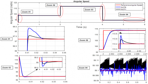
Figure 14 illustrates the rotor speed response using the improved NLPI controller under a step wind profile.
5.2.2 Variable wind profile results
Figure 15 shows the rotor speed response under a variable wind profile using the improved NLPI controller.
A comparison study between the results obtained with NLPI1 and NLPI6 controllers under step and variable wind profile is presented in the table below:
Table 4. Comparison of values between NLPI and NLPI6 under step wind
|
Controller |
Error |
Response Time (s) |
Overshoot (rad/s) |
|
NLPI1 |
0.0007994 |
0.075 |
0.36 |
|
NLPI6 (Eq 21) |
4.315e-6 |
0.0315 |
1.1475 |
The simulation results, presented in Table 4 and Figures 14 and 15 under variable and step wind profiles, demonstrate the effectiveness of the arctan function in reducing the response time to 0.075 seconds and the steady-state error to 4.315e-6. However, in terms of overshoot, NLPI6 shows reduced robustness. The following section proposes optimization to address this issue and improve performance using various metaheuristic algorithms. These algorithms include the widely cited PSO, the HHO, and the new GJO algorithm.
5.3 Simulation 3: The NLPI6 controller with optimization
In order to optimize the rotor speed, various metaheuristic algorithms, including PSO, HHO, and GJO were employed to adjust the NLPI6 controller’s parameters. The population size and the number of iterations were set to (100, 100) for PSO, (40, 40) for HHO, and (150, 150) for GJO, respectively. These configurations were carefully selected to ensure a suitable trade-off between computational efficiency and convergence reliability. The optimized parameter sets obtained with each algorithm are presented in Table 5.
Table 5. Different parameters obtained from each algorithm
|
Controller |
Kp0 |
Kp1 |
Kp2 |
Ki0 |
Ki1 |
Ki2 |
α1 |
α2 |
α3 |
|
PSO-NLPI6 |
19.9401 |
0.01 |
7.3875 |
/ |
25.6607 |
0.0711 |
2.5333 |
/ |
/ |
|
HHO-NLPI6 |
211.2479 |
1.7536 |
0.6116 |
/ |
33.5091 |
0.1028 |
28.1292 |
/ |
/ |
|
GJO-NLPI6 |
247.1343 |
36.8943 |
0.0169 |
/ |
24.1377 |
0.0126 |
33.0993 |
/ |
/ |
Figure 16. The rotor speed with NLPI controller optimized by HHO, PSO, GJO and step wind profile
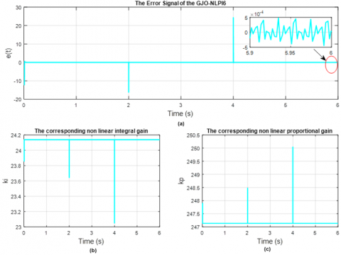
Figure 17. (a) The error signal curve of the GJO_NLPI6, (b) The proportional nonlinear gain of the GJO-NLPI6, (c) The integral nonlinear gain of the GJO-NLPI6
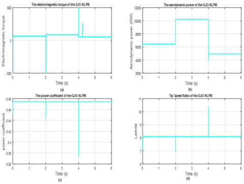
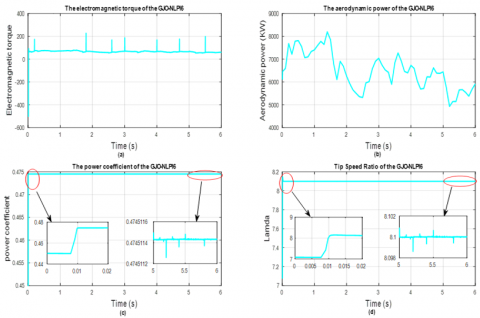
Figure 18. (a) The electromagnetic curve of the GJO-NLPI6, (b) The aerodynamic power curve of the GJO-NLPI6, (c) The power coefficient using the GJO-NLPI6, (d) The tip speed ratio using the GJO-NLPI6
Figure 19. The rotor speed with NLPI controller optimized by HHO, PSO, GJO and variable wind profile
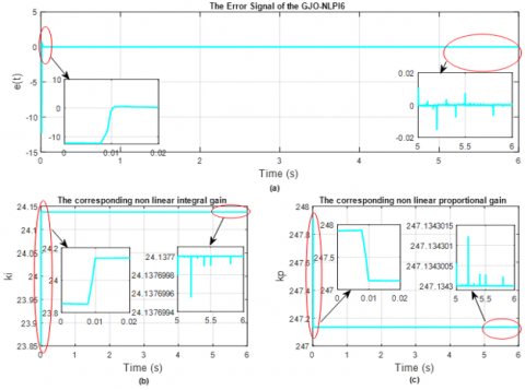
Figure 20. (a) The error signal curve of the GJO_NLPI6, (b) The proportional nonlinear gain of the GJO-NLPI6, (c) The integral nonlinear gain of the GJO-NLPI6
Figure 21. (a) The electromagnetic curve of the GJO-NLPI6, (b) The aerodynamic power curve of the GJO-NLPI6, (c) The power coefficient using the GJO-NLPI6, (d) The tip speed ratio using the GJO-NLPI6
Table 6. Comparison of values between different NLP6 controllers without and with optimization
|
Chapter 1 Controller |
Chapter 2 Error |
Chapter 3 Response Time (s) |
Chapter 4 Overshoot (rad/s) |
Chapter 5 AIE |
|
Chapter 6 NLPI6 |
Chapter 7 4.315e-6 |
Chapter 8 0.0315 |
Chapter 9 1.1475 |
Chapter 10 / |
|
Chapter 11 PSO-NLPI6 |
Chapter 12 0.0007026 |
Chapter 13 0.2 |
Chapter 14 2.89 |
Chapter 15 259.4841 |
|
Chapter 16 HHO-NLPI6 |
Chapter 17 0.0001829 |
Chapter 18 0.03 |
Chapter 19 0.75 |
Chapter 20 229.9707 |
|
Chapter 21 GJO-NLPI6 |
Chapter 22 3.15e-6 |
Chapter 23 0.0322 |
Chapter 24 0.0576 |
Chapter 25 225.4774 |
5.3.1 Step wind profile results
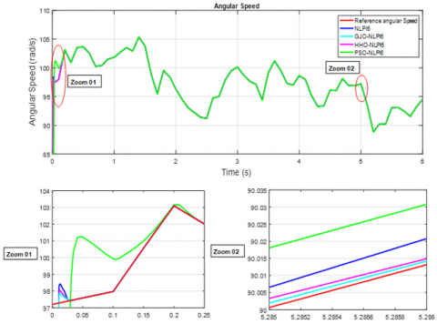
The rotor speed response under a step wind profile using the optimized NLPI controller tuned with PSO, HHO, and GJO algorithms is shown in Figure 16.
The following graphic displays the error curve of the optimal controller, GJO-NLPI6, which yields the best results for angular speed. It also shows the corresponding variations in the nonlinear proportional and integral gains required to achieve this minimal error under a step wind profile.
The electromagnetic torque, aerodynamic power, power coefficient, and tip speed ratio simulated under a step wind profile are presented in the Figure below.
5.3.2 Variable wind profile results
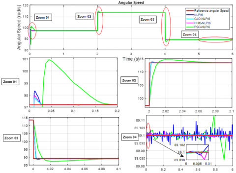
Figures 15 and 19, using PSO, HHO and GJO algorithms, demonstrate high efficiency and robustness. Among these, the GJO algorithm stands out with a remarkably low steady-state error of 3.15e-6, a fast settling time of 0.0322 s, and a minimal overshoot of 0.0576.
The results achieved with the optimal gains, as presented in Figures 17 and 20, are highlighted in green. The optimization results presented in Table 6, as well as the error curves of the GJO_NLPI6 represented in figures 17 and 20, highlighting the variations in the nonlinear proportional and integral gains required to achieve minimal error under step and variable wind profiles. It is observed that an increase in the Kp gain and a decrease in the Ki gain were necessary to reach a minimal error of 3.15e-6. Moreover, the fluctuations in the error are correlated with variations in the nonlinear Kp and Ki gains, emphasizing the importance of these dynamic adjustments in improving system performance.
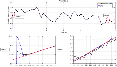
Figure 18, illustrates the variation in generated electromagnetic torque and aerodynamic power for both step and variable wind profiles. In these scenarios, the Cp reaches a value of 0.4745, while the TSR (λ) is 8.1. The electromagnetic torque fluctuates in reaction to the wind's dynamic nature, as the control mechanism adjusts to ensure optimal power extraction. As the wind profile modifications, so does the aerodynamic power, demonstrating the system's efficiency in capturing wind energy. Figure 19 illustrates the rotor speed response under a variable wind profile using the optimized NLPI controller tuned with PSO, HHO, and GJO algorithms.
Further insights into the performance of the best configuration, GJO-NLPI6, are provided in Figures 20 and 21. Specifically, Figure 20 presents (a) the error signal curve, (b) the proportional nonlinear gain, and (c) the integral nonlinear gain, highlighting the controller’s adaptability to dynamic operating conditions. Where Figure 21 depicts key performance indicators for the GJO-NLPI6 controller: (a) the electromagnetic torque, (b) the aerodynamic power, (c) the power coefficient, and (d) the tip-speed ratio. Table 6 summarizes the results obtained with NLPI6 without and with optimization controllers under a step and variable wind profile.
This study presented a wind turbine mathematical representation built with MATLAB/Simulink. Two types of wind speed profiles, variable, and step wind profiles, were studied to analyze the robustness of the NLPI controller. A comparison between different nonlinear PI controllers and the classical PI controller was conducted, demonstrating that the NLPI controller offers a more efficient response and robustness compared to the traditional PI controller. To enhance the robustness of the NLPI, a nonlinear arctan function was integrated into the controller's integral term, reducing the static error to 3.15e-6 and achieving a settling time of 0.0322 seconds. However, a slight overshoot of 0.0576 rad/s remained. To address this issue and further improve the controller's robustness, optimization using various metaheuristic algorithms, such as PSO, HHO, and GJO, was proposed. The optimization results were remarkable, particularly with the GJO algorithm, which demonstrated exceptionally robust performance. Its performance was significantly superior to the other algorithms tested, making it an optimal choice for wind turbine control systems. The simulations highlighted the potential of combining advanced nonlinear functions with metaheuristic optimization algorithms to significantly improve the control system's performance in both scenarios studied. The obtained results will be validated in future work through an experimental prototype of a Wind Energy Conversion System, where different robustness tests will be conducted to further assess the controller’s performance under realistic operating conditions.
The researchers extend their sincere gratitude to the Deanship of Scientific Research at the Islamic University of Madinah for the support provided to the Post-Publishing Program.
[1] Akbari, M.A., Aghaei, J., Barani, M. (2017). Convex probabilistic allocation of wind generation in smart distribution networks. IET Renewable Power Generation, 11(9): 1211-1218. https://doi.org/10.1049/iet-rpg.2017.0100
[2] Tyagi, A., Bihari, S.P., Chaurasia, G.S., Singh, A.P. (2025). An optimized controller for novel asymmetrical 51-level inverter in hybrid solar and wind turbine-connected power system. Electrical Engineering, 107(4): 4959-4977. https://doi.org/10.1007/s00202-024-02799-6
[3] Bouchemal, B., Chemachema, M. (2025). Model-free control for variable-speed wind energy conversion systems based on power tracking. Electrical Engineering, 107(1): 179-189. https://doi.org/10.1007/s00202-024-02514-5
[4] Njiri, J.G., Söffke, D. (2016). State-of-the-art in wind turbine control: Trends and challenges. Renewable and Sustainable Energy Reviews, 60: 377-393. https://doi.org/10.1016/j.rser.2016.01.110
[5] Baroudi, J.A., Dinavahi, V., Knight, A.M. (2007). A review of power converter topologies for wind generators. Renewable Energy, 32(14): 2369-2385. https://doi.org/10.1016/j.renene.2006.12.002
[6] Duran, M.J., Barrero, F., Pozo-Ruz, A., Guzman, F., Fernandez, J., Guzman, H. (2013). Understanding power electronics and electrical machines in multidisciplinary wind energy conversion system courses. IEEE Transactions on Education, 56(2): 174-182. https://doi.org/10.1109/TE.2012.2207119
[7] Kumar, D., Chatterjee, K.A. (2016). A review of conventional and advanced MPPT algorithms for wind energy systems. Renewable and Sustainable Energy Reviews, 55: 957-970. https://doi.org/10.1016/j.rser.2015.11.013
[8] Cheng, M., Zhu, Y. (2014). The state of the art of wind energy conversion systems and technologies: A review. Energy Conversion and Management, 88: 332-347. https://doi.org/10.1016/j.enconman.2014.08.037
[9] Singh, M., Chandra, A. (2011). Application of adaptive network-based fuzzy inference system for sensorless control of PMSG-based wind turbine with nonlinear-load-compensation capabilities. IEEE Transactions on Power Electronics, 26(1): 165-175. https://doi.org/10.1109/TPEL.2010.2054113
[10] Orlando, N.A., Liserre, M., Mastromauro, R.A., Dell'Aquila, A. (2013). A survey of control issues in PMSG-based small wind-turbine systems. IEEE Transactions on Industrial Informatics, 9(3): 1211-1221. https://doi.org/10.1109/TII.2013.2272888
[11] Hossain, M.M., Ali, M.H. (2015). Future research directions for the wind turbine generator system. Renewable and Sustainable Energy Reviews, 49: 481-489. https://doi.org/10.1016/j.rser.2015.04.126
[12] Buehring, I.K., Freris, L.L. (1981). Control policies for wind-energy conversion systems. IEE Proceedings C Generation Transmission and Distribution, 128(5): 253-261. https://doi.org/10.1049/ip-c.1981.0043
[13] Pao, L.Y., Johnson, K.E. (2009). A tutorial on the dynamics and control of wind turbines and wind farms. American Control Conference, St. Louis, MO, USA, pp. 2076-2089. https://doi.org/10.1109/ACC.2009.5160195
[14] Hua, G., Geng, Y. (2006). A novel control strategy of MPPT taking dynamics of wind turbine into account. In 2006 37th IEEE Power Electronics Specialists Conference, Jeju, Korea (South), pp. 1-6. https://doi.org/10.1109/pesc.2006.1712240
[15] Morimoto, S., Nakayama, H., Sanada, M., Takeda, Y. (2005). Sensorless output maximization control for variable-speed wind generation system using IPMSG. IEEE Transactions on Industry Applications, 41(1): 60-67. https://doi.org/10.1109/TIA.2004.841159
[16] Zhao, Y., Wei, C., Zhang, Z., Qiao, W. (2013). A review on position/speed sensorless control for permanent-magnet synchronous machine-based wind energy conversion systems. IEEE Journal of Emerging and Selected Topics in Power Electronics, 1(4): 203-216. https://doi.org/10.1109/JESTPE.2013.2280572
[17] Abdullah, M.A., Yatim, A.H.M., Tan, C.W., Saidur, R. (2012). A review of maximum power point tracking algorithms for wind energy systems. Renewable and Sustainable Energy Reviews, 16(5): 3220-3227. https://doi.org/10.1016/j.rser.2012.02.016
[18] Moor, G.D., Beukes, H.J. (2011). Maximum power point trackers for wind turbines. Renewable Energy, 36(10): 2655-2662. https://doi.org/10.1016/j.renene.2010.04.028
[19] Kaoutar, D., El Mahfoud, B., Brahim, B., Mohamed, A., Belkasem, I., Sana, M., Mohamed, B. (2023). Hybrid MPPT Control: P&O and Neural Network for Wind Energy Conversion System. Journal of Robotics and Control (JRC), 4(1): 2715-5072. https://doi.org/10.18196/jrc.v4i1.16770
[20] Salma, A., El-mahjoub, B., Ismail, B. (2019). Intelligent proportional-integral sliding mode control of wind turbine systems based particle swarm optimisation. International Journal of Automation and Control, 13(3): 347-373. https://doi.org/10.1504/IJAAC.2019.098585
[21] Belkacem, B., Noureddine, B., Lahouari, A.K., Ahmed, A. (2022). Fuzzy optimization strategy of the Maximum Power Point Tracking for a variable wind speed system. International Journal of Electrical and Computer Engineering (IJECE), 12(4): 4264-4275. http://doi.org/10.11591/ijece.v12i4.pp4264-4275
[22] Mohammad, B.T., Muhammad, K.A., Ali, M. (2021). Enhanced performance of PMSG in WECS using MPPT - fuzzy sliding mode control. Journal Européen des Systèmes Automatisés, 54(1): 85-96. https://doi.org/10.18280/jesa.540110
[23] Benkada, A., Chaikhy, H., Monkade, M. (2018). MPPT control for wind energy conversion system based on a T-S fuzzy. International Journal of Power Electronics and Drive System (IJPEDS), 9(2): 811-819. http://doi.org/10.11591/ijpeds.v9.i2.pp811-819
[24] Tian, Y.C., Tadé, M.O., Tang, J. (1999). A nonlinear PID controller with applications. IFAC Proceedings Volumes, 32(2): 2657-2661 https://doi.org/10.1016/S1474-6670(17)56452-6.
[25] Shi, X., Zhao, H., Fan, Z. (2023). Parameter optimization of nonlinear PID controller using RBF neural network for continuous stirred tank reactor. Measurement and Control, 56(9-10): 1835-1843. https://doi.org/10.1177/00202940231189307
[26] Luay, T.R., Noor, Q.Y., Saba, A. (2023). Performance of the optimal nonlinear PID controller for position control of antenna azimuth position system. Mathematical Modelling of Engineering Problems, 10(1): 366-375. https://doi.org/10.18280/mmep.100143
[27] Su, Y.X., Dong, S., Duan, B.Y. (2005). Design of an enhanced nonlinear PID controller. Mechatronics, 15(8): 1005-1024 https://doi.org/10.1016/j.mechatronics.2005.03.003
[28] Mehmet, K., Ömer, A., Hüseyin, D. (2012). Design and performance comparison of variable parameter nonlinear PID controller and genetic algorithm based PID controller. In 2012 International Symposium on Innovations in Intelligent Systems and Applications, Trabzon, Turkey, pp. 1-5. https://doi.org/10.1109/INISTA.2012.6246935
[29] Ruderman, M. (2025). Nonlinear integral extension of PID control with improved convergence of perturbed second-order dynamic systems. Advanced Control for Applications: Engineering and Industrial Systems, 7(2): e70017. https://doi.org/10.48550/arXiv.2404.02502
[30] Vijay, M., Himanshu, Ch., Asha, R., Vijander, S. (2018). Robust self-tuning fractional order PID controller dedicated to nonlinear dynamic system. Journal of Intelligent & Fuzzy Systems, 34(3): 1467-1478. https://doi.org/10.3233/JIFS-169442
[31] Homayoun, S. (1998). A new class of nonlinear PID controllers with robotic applications. Journal of Robotic Systems, 15(3): 161-181. https://doi.org/10.1002/(SICI)1097 4563(199803)15:3<161::AID-ROB4>3.0.CO;2-O
[32] Xu, Y., Hollerbach, J.M., Ma, D. (1995). A nonlinear PD controller for force and contact transient control. IEEE Control Systems Magazine, 15(1): 15-21. https://doi.org/10.1109/37.341859
[33] AL-Samarraie, S.A., Abbas, Y.K. (2012). Design of electronic throttle valve position control system using nonlinear PID controller. International Journal of Computer Applications, 59(15): 27-34. https://doi.org/10.5120/9625-4273
[34] Hazzab, A., Gouabi, H., Habbab, M., Rezkallah, M., Ibrahim, H., Chandra, A. (2023). Wind turbine emulator control improvement using nonlinear PI controller for wind energy conversion system: Design and real-time implementation. International Journal of Adaptive Control and Signal Processing, 37(5): 1151-1165. https://doi.org/10.1002/acs.3566
[35] Ren, Y., Li, L., Brindley, J., Jiang, L. (2016). Nonlinear PI control for variable pitch wind turbine. Control Engineering Practice, 50: 84-94 https://doi.org/10.1016/j.conengprac.2016.02.004.
[36] Liu, J., Zhou, F., Zhao, C., Wang, Z. (2019). A PI-type sliding mode controller design for PMSG-based wind turbine. Complexity, 2019(1): 2538206. https://doi.org/10.1155/2019/2538206
[37] Charrak, H. (2025). Recent advances in stability and seepage analysis of earth dams: A review leveraging numerical methods and computational intelligence. Islamic University Journal of Applied Sciences, VII(1): 258-265. https://doi.org/10.63070/jesc.2025.016
[38] Arabi, M., Zennir, Y., Bourourou, F. (2023). Wind turbine mechanical speed regulation reliability of artificial intelligent PSO-FLC control. In 2023 International Conference on Electrical Engineering and Advanced Technology (ICEEAT), Batna, Algeria, pp. 1-5.
[39] Chetioui, L., Zennir, Y., Arabi, M., Schulte, H., Mechhoud, El.A., Bendib, R. (2023). Optimization of a speed controller of a WECS with metaheuristic algorithms. In Proceedings of the 2nd International Conference on Computational Engineering and Intelligent Systems, Boumerdes, Algeria, 29(1): 7. https://doi.org/10.3390/engproc2023029007
[40] Ouguissi, H., Saadi, S., Benmessaoud, H.E., Abdelaziz Rabehi, A. (2025). Chua chaotic system parameters estimation using PSO algorithm to increase its dynamics. Islamic University Journal of Applied Sciences (IUJAS), VII(1): 138-148. https://doi.org/10.63070/jesc.2025.009.
[41] Chetioui, L., Zennir, Y., Arabi, M., Schulte, H., Bendib, R , Mechhoud, El.A. (2023). (2023). Optimization of a speed controller of a DFIM with metaheuristic algorithms. Engineering Proceedings, 29(1): 13. https://doi.org/10.3390/engproc2023029013
[42] Chopra, N., Ansari, M.M. (2022). Golden jackal optimization: A novel nature-inspired optimizer for engineering applications. Expert Systems with Applications, 198: 116924. https://doi.org/10.1016/j.eswa.2022.116924
[43] Conadini, M.L., Ippoliti, G., Orlando, G. (2013). Fully sensorless robust control of variable-speed wind turbines for efficiency maximization. Automatica, 49(10): 3023-3031. https://doi.org/10.1016/j.automatica.2013.07.028
[44] Ali, R.B., Schulte, H., Mami, A. (2017). Modeling and simulation of a small wind turbine system based on PMSG generator. 2017 Evolving and Adaptive Intelligent Systems (EAIS), Ljubljana, Slovenia, pp. 1-6. https://doi.org/10.1109/EAIS.2017.7954833.
[45] Knight, A.M., Peters, G.E. (2005). Simple wind energy controller for an expanded operating range. IEEE Transactions on Energy Conversion, 20(2): 459-466. https://doi.org/10.1109/TEC.2005.847995
[46] Larabi, M.S., Yahmedi, S., Zennir, Y. (2022). Robust LQG controller design by LMI approach of a doubly-fed induction generator for aero-gen. Journal Européen des Systèmes Automatisés, 55(6): 803-816. https://doi.org/10.18280/jesa.550613
[47] Kooning, J.G.L., Vyver, J., Vandoorn, T.L., Vandevelde, L. (2013). Online estimation of the power coefficient versus tip-speed ratio curve of wind turbines. In IECON 2013 - 39th Annual Conference of the IEEE Industrial Electronics Society, Vienna, Austria, pp. 1792-1797. https://doi.org/10.1109/IECON.2013.6699403
[48] Nasiri, M., Milimonfared, J., Fathi, SH. (2014). Modeling, analysis and comparison of TSR and OTC methods for MPPT and power smoothing in Permanent Magnet Synchronous Generator-based wind turbines. Energy Conversion and Management, 86: 892-900. https://doi.org/10.1016/j.enconman.2014.06.055.
[49] Kennedy, J., Eberhart, R. (1995). Particle swarm optimization. In Proceedings of ICNN'95 - International Conference on Neural Networks, Perth, WA, Australia, pp. 1942-1948. https://doi.org/10.1109/ICNN.1995.488968
[50] Heidari, A.A., Mirjalili, S., Faris, H., Aljarah, I., Mafarja, M., Chen, H. (2019). Harris hawks optimization: Algorithm and applications. Future Generation Computer Systems, 97: 849-872. https://doi.org/10.1016/j.future.2019.02.028
[51] Billel, M., Abdallah, S., Djalel, D., Yassine, A. (2015). Effective MPPT technique and robust power control of the PMSG wind. IEEJ Transactions on Electrical and Electronic Engineering, 10: 619-627. https://doi.org/10.1002/tee.22128