Loubna Khellaf*![]() | Adel Djellal
| Adel Djellal![]() | Hichem Mayache
| Hichem Mayache![]()
© 2025 The authors. This article is published by IIETA and is licensed under the CC BY 4.0 license (http://creativecommons.org/licenses/by/4.0/).
OPEN ACCESS
Despite the promising potential of photovoltaic energy and its wide range of uses, it still has shortcomings today, mainly due to its highly sensitive nature to environmental factors, resulting in low efficiency and energy loss. Therefore, the implementation of a robust control strategy for photovoltaic systems becomes essential in order to efficiently track the maximum power point (MPP) and deliver the best possible performance. This study proposes the implementation of a non-linear Proportional-Integral (NPI) controller in a PV system with a resistive load. The NPI controller is designed by integrating a non-linear gain function based on Popov’s stability criterion into the classical PI structure, aligning with the nonlinear characteristics of PV systems. Furthermore, intelligent control techniques, in particular these metaheuristic algorithms: Particle Swarm Optimization (PSO), Genetic Algorithm (GA) and Grey Wolf optimizer (GWO), were utilized to fine-tune both non-linear PI and classic PI controllers. The performance of the proposed approach is assessed using key metrics such as Mean Square Error (MSE), overshoot, settling time, and efficiency, demonstrating its effectiveness in enhancing PV system operation.
metaheuristic algorithm, Particle Swarm Optimization, Grey Wolf Optimization, Genetic Algorithm, optimization, artificial intelligence, PV system, nonlinear PID
Photovoltaic energy has received particular attention in recent years due to its sustainability and wide range of applications, including stand-alone systems, grid-connected installations and small-scale uses such as street lighting [1, 2]. However, the efficiency of photovoltaic systems is very sensitive and highly dependent on environmental factors, including irradiation and temperature, which can significantly reduce energy production and lead to energy losses [3].
In such circumstances, traditional MPPT methods such as perturbation and observation (P&O) and incremental conductance (InC) often offer limited performance and numerous ripples [4]. Consequently, achieving reliable performance of photovoltaic systems under these specific conditions is still a critical challenge in ongoing research.
To overcome these limitations in photovoltaic systems, the integration of a robust control loop is essential for regulating output and enhancing overall system performance. Among the most commonly used techniques is the PID controller, widely recognized for its effectiveness, simplicity, and ease of implementation [5].
However, one of the main drawbacks of PID controllers is to properly choose a suitable and correct control gains to get the best possible performance [6], which is even trickier in non-linear systems such as photovoltaics. Various techniques are available for this purpose, such as manual tuning, Ziegler and Nichols, and more recent ones introducing artificial intelligent computing [7].
While recent strategies offer notable advantages, they are also associated with certain trade-offs. Consequently, there is a growing interest on artificial-intelligence-based methods and soft computing techniques along with optimization algorithms in enhancing solar PV panels and to cope with the system's inherent nonlinear behavior. However, despite the effectiveness of AI-based techniques such as the Fuzzy Logic Controller (FLC) and Artificial Neural Networks (ANN) in achieving high tracking performance, they often struggle under conditions of strong nonlinearities, particularly during partial shading. As a result, these methods are prone to stagnation at local power points, exhibit prolonged settling times, and suffer from reduced tracking accuracy.
Moreover, it is worth mentioning that the combination of these methods is also considered a go-to solution to mitigate the limitations of both strategies, offering very efficient tracking of MPP and GMPP in partial shading scenarios. Many maximum power point tracking algorithms (MPPT) techniques was discussed and summarized in the study [8], evaluated under both uniform and partial shading scenarios.
To meet this challenge, several techniques have been used, based on well-known classical techniques and on more recent intelligence-based techniques. An intelligent control technique combining an SPSOA MPPT algorithm with a non-linear NPID controller and compared to a conventional technique such as a conventional PID controller was proposed in the study [9], the results showed a reduction in power losses and an increase in PV system reliability as the proposed control outperformed other techniques. In the study [10], an intelligent self-adaptive MPPT strategy based on the integration of Adaptive Neuro-Fuzzy Inference System (ANFIS) with PSO optimization to enhance energy extraction efficiency. The proposed approach was evaluated under a variety environmental condition, demonstrating MPPT efficiencies of 99.2% under uniform irradiation and 98.7% under dynamically changing conditions, outperforming conventional MPPT algorithms Notably, the proposed ANFIS-PSO technique can avoid the local power maxima under partial shading scenarios by accurately identifying the point of maximum overall power. Overall, the approach significantly improved energy tacking efficiency with minimal grid disturbances, and enhanced the robustness of the PV system. In addition, for parameter optimization, a hybrid GA-PSO algorithm was used for both controllers, resulting in improved system stability. In the study conducted by Malarvili and Mageshwari [11] a modified nonlinear PID controller was formulated in compliance with the Popov criterion, ensuring system hyperstability for both MPPT control and the regulation of a single-stage single-phase (SSSP) grid-connected inverter in a photovoltaic system. The proposed approach demonstrated enhanced MPPT performance, characterized by rapid convergence and reduced oscillations around the maximum power point. Furthermore, the nonlinear PID controller exhibited improved effectiveness in inverter control, achieving a total harmonic distortion (THD) of less than 0.5%, minimizing energy losses through accurate MPP tracking, and maintaining a unity power factor on the grid side. A nonlinear control strategy was proposed in the study [12] for regulating current and voltage in a photovoltaic (PV) system integrated into a microgrid. The study presented a comparative analysis between the nonlinear PI (NPI) controller and a conventional PI controller. The proposed method employs a variable nonlinear gain function that dynamically adjusts according to the system error. when the error is large, the gain increases to accelerate the convergence toward the reference, while near the desired value, it decreases to ensure smooth tracking. This adaptive mechanism effectively suppresses high-frequency oscillations and reduces the settling time by stabilizing the system more rapidly. Furthermore, simulation results demonstrated a notable improvement in performance, with a consistent reduction in the Integral of Absolute Error (IAE) across all tested scenarios. In the study [13], the PID controller gains are optimized using the Particle Swarm Optimization (PSO) algorithm and compared to those obtained through the Cohen-Coon method. The results demonstrate that the PSO-optimized PID controller significantly enhances both transient and steady-state performance, achieving a settling time of 2.37 s and an overshoot of 0.78%, compared to 6.12 s and 20.14% with the Cohen-Coon method. These findings underscore the advantages of incorporating artificial intelligence techniques in control system design. Overall, PSO-tuned controllers were shown to outperform the Cohen-Coon method in all areas. In the study [6], the Gorilla Troops Optimizer (GTO) algorithm was used to fine-tune the PID controller gains. Four types of error evaluation indicators were used: integral absolute error (IAE), integral time absolute error (ITAE), integral square error (ISE) and integral time square error (ITSE). The results showed that soft computing tools provide better results when tuning the gain of PID controllers than more traditional methods such as Z-N tuning. In addition, GTO showed promising results in terms of rise time, stability and settling time, as well as minimum steady-state error. In the study [14], introduced a teaching-learning-based optimization TLBO to optimize the parameter of a fractional order PID (FOPID) controller in a grid connected PV system, simulation results showed the effectiveness of the proposed control strategy with better dynamic response and outperforming other techniques. Finally, in the study [15] GWO was used to adjust the converter duty cycle to maximize output power, resulting in greater stability and rapid convergence with less oscillation. A 43.6% improvement in output power was observed compared to the situation without MPPT.
Improving the performance of photovoltaic systems remains a persistent challenge despite academic research, and the various existing conventional strategies have known limitations. To fill this persistent gap, nonlinear PID controllers comes as a viable answer. As an extended version of conventional PID controllers, they are characterized by additional non-linear gain cascaded with the conventional structure, they offer more flexibility and better alignment with the inherently nonlinear nature of PV systems, thereby making them ideally suited for such applications. Furthermore, tuning the parameters of such controllers is essential to achieve maximum system efficiency. Among the many existing algorithms, Genetic Algorithm (GA), Particle Swarm Optimization (PSO) and Grey Wolf Optimizer (GWO) have enjoyed remarkable success in various applications.
This paper is organized as follows: Section 2 presents the description of the photovoltaic system and behavior analysis. Section 3 deals with the design of the NPID controller. Optimization algorithms and the fitness function used in this work are carried out in Sections 4 and 5 respectively. The results, along with performance evaluations, are discussed in Section 6. The concluding remarks are provided in Section 7.
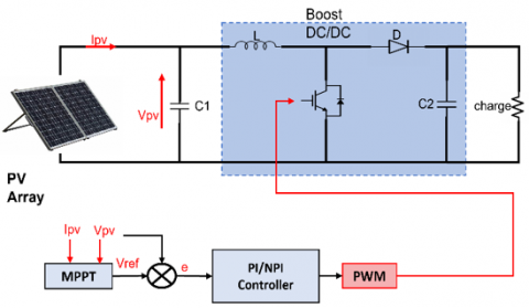
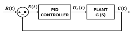
The complete system is consisted of a PV array for solar energy conversion, boost DC/DC converter connected to a resistive load and a MPPT algorithm with controller. The conception of the PV system is presented in Figure 1.
Figure 1. PV system control configuration
The array is composed of multiple identical PV modules connected in a combination of series and parallel to achieve the desired voltage and current levels. For this work, a Solar Power Industries SPI-M210-60 PV Panel was utilized in this study, PV array is consisted of 10 modules in series and 40 in parallel to supply an 83.9 kW output power under standard test conditions (STC), i.e., solar radiation of 1000 W/m2, and a temperature of 25℃. Details are found in Table 1.
Table 1. PV array specifications
|
Parameter |
Value |
|
Rated power per module |
209.8 W |
|
Number of modules in series |
10 |
|
Number of modules in parallel |
40 |
|
Pv array maximum power |
83.9 kW |
|
Pv array Mpp voltage/current |
289 V / 290.4 A |
|
Open circuit voltage/ short circuit current |
364 V / 316.4 A |
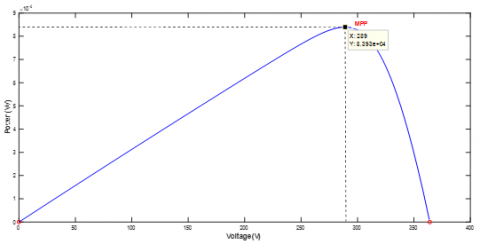
In order to comprehend the non-linear dynamic of the PV system, an analyze of the influence of abrupt variations of environmental conditions is conducted. Figure 2 to Figure 4 present the P-V and I-V characteristics of PV array under different conditions.
(a) P-V
(b) I-V
Figure 2. Characteristics of PV array under STC
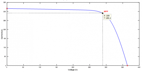
(a) P-V
(b) I-V
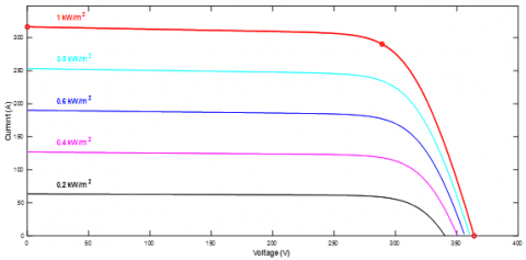
Figure 3. Characteristics of PV array under various irradiance levels
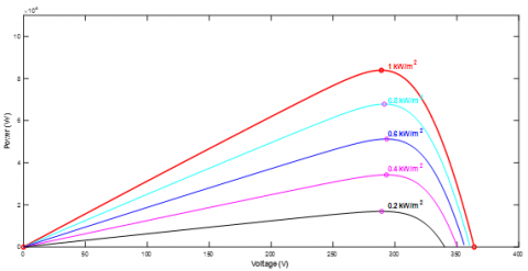
(a) P-V
(b) I-V
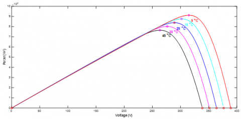
Figure 4. Characteristics of PV array under various temperature levels
Figure 2 presents the P-V and I-V characteristic under Standard Test Conditions (STC) which are 1000 W/m2 of irradiance and temperature of 25℃.
Figure 3 depicts the P-V and I-V characteristic when temperature is at 25℃ and different levels of irradiance set at 200 W/m2 and 1000 W/m2.
As can be seen, when irradiance increases, delivered current increases and so generated power, and voltage varies very slightly. Thus, maximum power point varies with important amounts.
In contrast, when irradiance is maintained at 1000 W/m2, and temperature varies between 5℃ and 45℃. When temperature increases voltage at maximum power point decreases leading to a reduction in the overall maximum power point. It is worth mention that the increase in irradiance and temperature have opposite influence on PV system, as depicted in Figure 4.
Tracking the maximum power point is the role of MPPT controllers, different techniques exist in both literature and industry.
Despite the widespread use and popularity of PID controllers for their robustness, they lack adaptability in non-linear systems such as photovoltaics due to abrupt changes in environmental operating conditions [16]. Non-linear PID controllers have been developed to overcome the shortcomings of conventional PID controllers. The typical PID controller is often expressed in its standard form, as employed in references [17, 18], acting on the error by means of three actions: proportional, integral and derivative, each weighted by a specific gain, Kp, Ki and Kd respectively, and is defined as follows:
$U_c(t)=\left(K_p E(t)+K_i \int E(t) d t+K_d \frac{d E(t)}{d t}\right)$ (1)
3.1 Design of non-linear gain – Popov’s hyper stability criterion
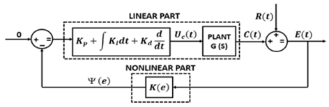
Non-linear PID controller is derived by introducing a non-linear hyperbolic cosine gain function in cascade with the conventional PID structure [11, 19]. Block diagrams are displayed in Figures 5 and 6.
The non-linear gain is designed based on the hyperstability criterion, which guarantees robust and global system stability [20]. Consequently, the output of the NPID controller is defined as follows:
$\begin{gathered}U_{-} c(t)=(K(e))\left(K_p E(t)+K_i \int E(t) d t\right. \left.+K_d \frac{d E(t)}{d t}\right)\end{gathered}$ (2)
$U_c(t)=(\psi(e))\left(K_p+K_i \int d t+K_d \frac{d}{d t}\right)$ (3)
Figure 5. Linear PID control block
Figure 6. Non-linear PID block diagram
Here, $K(e)$ denotes the nonlinear gain, and $\Psi(e)$ is a nonlinear transformation of the error signal, defined as:
$\psi(e)=(K(e) \times E(t))$ (4)
Figure 7. Hyper stable nonlinear PID block diagram
Illustration of a modified hyper stable nonlinear PID controller is shown in Figure 7.
The non-linear gain is designed based on Popov’s criterion, which states global asymptotic stability if both of the following conditions are satisfied:
For the nonlinear part:
$\eta\left(t_0, t_1\right)=\int_{t_0}^{t_1} E(t) \psi(e) d t \geq-\gamma_0^2 \forall t_1 \geq t_0$ (5)
where, $\gamma_0^2$ is a positive finite constant, and for the linear part:
The transfer function $\left(K_p+K_i \int d t+K_d \frac{d}{d t}\right)\left(\frac{C(t)}{U_c(t)}\right)$ must be strictly positive real by Kalman-Yakubovich-Lemma.
By inserting (4) in (5), we derive:
$\begin{array}{r}\eta\left(t_0, t_1\right)=\int_{t_0}^{t_1} E(t) K(e) E(t) d t \geq-\gamma_0^2 \quad \forall t_1 \geq t_0\end{array}$ (6)
To satisfy the inequality (6), $K(e)$ could be in any form of nonlinear function of error $E(t)$ that is bounded in the range $0 \leq K(e) \leq K_{\max }$.
To efficiently design the nonlinear gain function, it is essential to analyze the closed-loop control behavior. During the transient phase, the error $E(t)$ is relatively large; therefore, $K(e)$ should also be large to accelerate the system's response. Conversely, in the steady-state phase, $E(t)$ becomes small, and $K(e)$ should decrease accordingly to minimize steadystate oscillations while maintaining accuracy. This adaptive adjustment ensures rapid convergence when the system experiences disturbances while preserving stability once it reaches the desired operating point.
As a result, the nonlinear gain $K(e)$ is defined as in (7), exhibiting a nonlinear dependence on the error and being proportional to an exponential function with base $\beta$.
$K(e)=K_0(\beta)^e$ where: $K_0, \beta \geq 0$ (7)
For $0<\beta<1$: the error is defined as
$e= \begin{cases}e, & e \geq-e_{\max } \\ -e_{\max }, & e<-e_{\max }\end{cases}$
For $\beta>1$
$e= \begin{cases}e, & e \leq e_{\max } \\ +e_{\max }, & e>e_{\max }\end{cases}$
$e_{\max }$ can be determined according to the dynamics of the system. Thus, by substituting Eq. (6) in Eq. (7):
$\begin{aligned} & \eta\left(t_0, t_1\right) & =\int_{t_0}^{t_1} E(t)\left[K_0(\beta)^e\right] E(t) d t & =\int_{t_0}^{t_1} E(t) K_0 \exp (e \ln (\beta)) E(t) d t \geq 0 \geq-\gamma_0^2\end{aligned}$ (8)
$K(e)$ is defined in $[0, \infty]$. From Eq. (8), we get:
$K(e)=K_0 \exp (e \ln (\beta))$ (9)
Inserting $\alpha=\ln (\beta)$ in Eq. (9), we obtain: $K(e)= K_0 \exp (\alpha e)$, with $K_0, \beta$ and $\alpha \geq 0$.
Hence, the nonlinear gain is specified separately for the two regions $\beta<1$ and $\beta>1$. As follows:
For $\beta=\exp (-\alpha)<1 ; K(e)$ is defined as:
$\begin{aligned} & K(e)=K_0 \exp (-\alpha e) \\ & =\left\{\begin{array}{cl}K_0 & e=0 \\ 0 & e \rightarrow+\infty: \text { lower bound } \\ K_0 \exp \left(\alpha e_{\max }\right) & e<-e_{\max }: \text { upper bound }\end{array}\right.\end{aligned}$
For $\beta=\exp (\alpha)>1$:
$\begin{aligned} & K(e)=K_0 \exp (\alpha e) \\ & =\left\{\begin{array}{cl}K_0 & e=0 \\ 0 & e \rightarrow-\infty: \text { lower bound } \\ K_0 \exp \left(\alpha e_{\max }\right) & e>+e_{\max }: \text { upper bound }\end{array}\right.\end{aligned}$
A limitation common to both expressions of $K(e)$ for regions $\beta<1$ and $\beta>1$ arises at their lower boundary, where the gain becomes inefficient. Specifically, as the error approaches large magnitudes ($\mathrm{e} \rightarrow \pm \infty$) the minimum gain reaches $K_{\min }=0$, causing the control action to lose the desired responsiveness. Therefore, an enhanced nonlinear gain formulation can be introduced by combining both of the two previous cases giving in hyperbolic cosine function to enhance performance while preserving the stability properties of the closed-loop system.
$K(e)=K_0 \frac{\exp (\alpha e)+\exp (-\alpha e)}{2}=K_0 \cosh (\alpha e)$ (10)
where,
$e=\left\{\begin{array}{cl}e, & |e| \leq e_{\max } \\ e_{\max } \operatorname{sign}(e), & |e|>e_{\max }\end{array}\right.$
$K(e)=\left\{\begin{array}{cl}K_0, & e=0 \\ K_0 \cosh \left(\alpha e_{\max }\right), & |e|>e_{\max }\end{array}\right.$
Metaheuristic algorithms are one tool among many that are being constantly developed in the artificial intelligence field. A great answer to real world problems, they are considered an effective optimization strategy as they offer great performance due to their high flexibility controller parameters tuning [21, 22].
Metaheuristic algorithms aim to enhance candidate solutions through iterative processes, exploring the search space using adaptive, nature-inspired strategies [23]. Their flexibility and robustness make them particularly suitable for solving complex, dynamic, and non-linear optimization problems [24].
Among the myriads of metaheuristic algorithms available, three distinct types stand out for their promising performance in this field: the GA [25-28], the particle swarm optimizer (PSO) [29-31] and, more recently, the gray wolf optimizer (GWO) [32-34].
4.1 Genetic Algorithm (GA)
The Genetic Algorithm (GA) is a stochastic optimization method inspired by the principles of natural selection and evolution. Renowned for its effectiveness in handling complex and nonlinear problems, GA simulates evolutionary processes through biologically inspired operators such as selection, crossover, and mutation. These mechanisms enable the algorithm to explore a wide solution space and progressively refine candidate solutions toward high-quality outcomes. Due to its robustness and adaptability, GA has been widely adopted in control systems engineering applications, extensively for optimizing the parameters of PID controllers, where it has gained significant interest in recent research. Step by step implementation of GA algorithm inspired from the study [35] is given as follows:
(a) Procedure:
•Set count for the number of generations; t=0.
•Create initial population of potential solutions randomly denoted as P(O).
•Each individual P(t) undergoes evaluation through a fitness function, t is the population index.
(b) If termination criteria are not satisfied do:
•t++
•Next generation is created
•Introduce crossover among a subset of the population t
•Mutation process for a portion of the population t
•Evaluation of the fitness for the next generation
(c) Return best solution
4.2 Particle Swarm Optimization (PSO)
Kennedy and Eberhart were the first to propose the Particle Swarm Optimization (PSO) algorithm in reference [36]. Its strategy is modeled after the collective patterns of sociobiological animal, such as flocks of birds, shoals of fish, and also bees, especially when searching for food, and how their unison leads to enhanced outcome [37].
In this approach, the search space is explored by particles that update their velocities and positions in response to both their own prior successes and the performance of their peers. The algorithm promotes collaboration among particles, allowing them to be influenced by the most successful individuals, which helps steer the entire swarm toward promising regions of the solution space [38]. These dynamics are mathematically governed by update equations (see Eqs. (11)-(12)), which balance exploration and exploitation. The swarm progressively refines its search, guided by each particle’s best-known position and the overall best solution found so far. PSO algorithm is given bellow [39]:
The mathematical formulation of the PSO algorithm, as utilized in reference [40], is governed by the following Eqs. (11) and (12):
$\begin{aligned} V_{-} i=\omega V_{i-1}+c_1 r_1 & \left(P_{\text {best }}-X_{i-1}\right) & +c_2 r_2\left(G_{\text {best }}-X_{i-1}\right)\end{aligned}$ (11)
$X_i=X_{i-1}+V_i$ (12)
where, $V_i$ represents the velocity of the particle, $X_i$ its position, $P_{\text {best }}$ the best position found by the particle, and $G_{\text {best }}$ the best position found by the entire population. The parameter $\omega$ denotes the inertia weight, $c_1$ and $c_2$ are acceleration coefficients, and $r_1, r_2$ are random values uniformly distributed in the range $(0,1)$.
4.3 Grey Wolf Optimization (GWO)
The Grey Wolf Optimizer (GWO) is a nature-inspired, population-based optimization technique that draws from the social structure and hunting behavior of grey wolves [41]. In the wild, these animals live in groups of 5 to 12 members, organized by a strict social hierarchy. Each wolf holds a rank (alpha, beta, delta, or omega) which determines its role in the pack. The alpha wolf, whether male or female, leads the group and is responsible for decision-making. GWO models this hierarchy to structure the optimization process, simulating the wolves’ natural strategy in hunting prey. This behavior is represented in three phases: tracking and chasing the prey, surrounding and pressuring it, and finally attacking [42]. These actions are mathematically expressed by:
$\vec{D}=\left|\vec{C} \cdot X_p(t)-\vec{X}(t)\right|$ (13)
$\vec{X}(t+1)=\overrightarrow{X_p}(t)-\vec{A} \cdot \vec{D}$ (14)
$\overrightarrow{X_p}(t)$ represents the target estimated position, corresponding to the current best solution, while $\vec{X}(t)$ denotes the position of the search agent - the grey wolf position, The coefficient vectors $\vec{A}$ and $\vec{C}$ are defined as follows:
$\vec{A}=2 \vec{a} \cdot \overrightarrow{r_1}-\vec{a}$ (15)
$\vec{c}=2 \overrightarrow{r_2}$ (16)
Here, the coefficient vector $\vec{a}$ decreases linearly from 2 to 0 throughout the iterations, while $\overrightarrow{r_1}$ and $\overrightarrow{r_2}$ are random vectors uniformly distributed in the interval [0,1]. The position of each search agent is updated according to the influence of the three leading solutions, which are alpha, beta, and delta and expressed as below:
$\vec{X}(t+1)=\frac{\overrightarrow{X_1}+\overrightarrow{X_2}+\overrightarrow{X_3}}{3}$ (17)
This mechanism effectively balances global exploration and local exploitation, allowing the Grey Wolf Optimizer to converge efficiently toward optimal solutions within complex and nonlinear search spaces.
GWO algorithm follows these steps:
Step 1. Initialize a population of search agents $X_i$, where i =1, 2..., n.
Step 2. Compute the initial coefficients a, A, and C using Eqs. (15) and (16).
Step 3. Evaluate the fitness of each agent and identify:
Xα: the best solution (alpha wolf)
Xβ: the second-best solution (beta wolf)
Xδ: the third-best solution (delta wolf)
To evaluate system performance, there are various processing criteria, whose aim is to minimize the error between the desired setpoint and the system output. They play a crucial role in guiding the algorithm towards the best solution. In the context of this research, the mean square error (MSE) cost function was chosen, along with metrics like: Maximum Overshoot (Mp), Steady State Error (ess), and Settling Time (ts).
The MSE calculates the mean square error and is defined as follows:
$M S E=\frac{1}{n} \sum_{i=1}^n(r(i)-y(i))^2$ (18)
$y(i)$ is the output voltage of PV array and $r(i)$ is the desired output voltage generated from MPPT algorithm.
Maximum Overshoot (Mp): maximum peak of the output $\left(x_{\text {peak}}\right)$ from the desired setpoint ($x_{\text {setpoint}}$) during a transient response. It is expressed in percentage (%) and calculated as follows:
$M_p=\frac{x_{\text {peak }}-x_{\text {setpoint }}}{x_{\text {setpoint }}} \times 100 \%$
Steady State Error (ess): difference between the output and the desired output (reference) during steady state.
Settling Time (ts): Time taken for the system to stay within a certain band (±5% in this work) of the setpoint.
To capture the trade-offs among various dynamic performance metrics, a weighted sum objective function is employed. This allows simultaneous minimization of error, overshoot, steady state error, and settling time:
$J=\omega_1 \times M S E+\omega_2 \times M_p+\omega_3 \times e_{s s}+\omega_4 \times t_s$
where, $\omega_1, \omega_2, \omega_3, \omega_4$ are the weighting coefficients assigned to each metric. In this study, the weights are set as follows: $\omega_1=0.4, \omega_2=0.2, \omega_3=0.2$, and $\omega_4=0.2$. They were selected to emphasize tracking accuracy through MSE, and balancing out the other metrics.
6.1 Response of PV system under standard test condition
In order to identify the most appropriate parameters for Genetic Algorithms (GA), Particle Swarm Optimization (PSO) and Gray Wolf Optimization (GWO), further analysis was carried out, and the outcomes are presented in Tables 2-4.
Table 2. Configuration of GA parameters
|
Parameter |
Value |
|
Population size |
30 |
|
Mutation Rate |
0.3 |
|
Crossover Rate |
0.7 |
|
Lower Bound |
0 |
|
Upper Bound |
1 |
|
Number of generations |
100 |
Table 3. Configuration of PSO parameters
|
Parameter |
Value |
|
Swarm Population size |
30 |
|
Inertia Weight ($\omega$) |
0.5 |
|
Cognitive Coefficient $\left(c_1\right)$ |
1 |
|
Social Coefficient $\left(c_2\right)$ |
2 |
|
Lower Bound |
0 |
|
Upper Bound |
1 |
|
Max Iteration |
100 |
Table 4. Configuration of GWO parameters
|
Parameter |
Value |
|
Number of Search Agents |
30 |
|
Lower Bound |
0 |
|
Upper Bound |
1 |
|
Max Iteration |
100 |
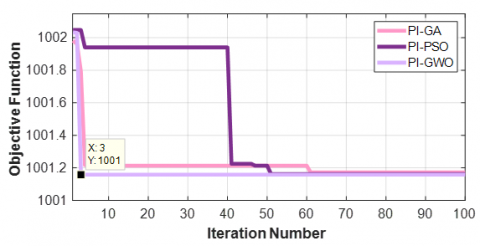
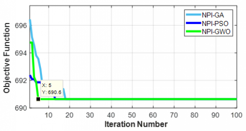
The objective function evolution graph is shown in Figure 8 for the PI controller and in Figure 9 for the NPI controller. As can be seen, the non-linear PI controller has the best optimal objective function value, 690.6, compared to the conventional PI controller, whose best objective fitness value is 1001. As far as the best algorithm performance is concerned, it is clear that the output of the Gray Wolf optimizer (GWO) is superior to that of the GA and the particle swarm optimizer in terms of convergence speed, since it could reach the lowest value faster with only 5 iterations for the NPI and 3 iterations for the conventional PI. It can therefore be said that the non-linear PI controller with the Gray Wolf optimizer improves the system's stability and time response, and has potentially the best overall performance. The tuned parameters are shown in the Table 5.
Figure 8. Convergence graph of PI controller objective function
Figure 9. Convergence graph of NPI controller objective function
Table 5. Tuned PI and NPI controller gains
|
Controller |
|
Kp |
Ki |
$\alpha$ |
$K_0$ |
|
PI |
ga |
0.6215 |
0.0108 |
- |
- |
|
pso |
0.6309 |
0.0229 |
- |
- |
|
|
gwo |
0.6153 |
0.00998 |
- |
- |
|
|
NPI |
ga |
0.4992 |
0.3872 |
0.0003 |
1 |
|
pso |
0.6001 |
0.3158 |
0.0195 |
0.8545 |
|
|
gwo |
0.8610 |
0.63759 |
0.0001 |
0.6045 |
Figure 10. Comparison of elapsed optimization times for PI and NPI controllers
Figure 10 shows that NPI-based controllers require longer optimization times than PI controllers, indicating higher computational complexity due to their nonlinear structure and additional gains. Among the algorithms, GA exhibits the highest elapsed time, while GWO achieves the lowest for PI tuning. Nevertheless, this increased computational demand in NPI controllers is offset by their superior control performance.
To demonstrate the importance of implementing a robust control loop in PV systems, including the application of artificial intelligence-based metaheuristic algorithms for fine tuning both PI controller and nonlinear PI controller (NPI), the tracking efficiency of each controller was evaluated and first tested under standard test condition (STC), i.e., under temperature of 25℃ and irradiance of 1000 W/m2. The results are shown in figures below. The system efficiency is evaluated under steady-state conditions using the following expression:
Efficiency $(\eta)=\frac{\text { Experiment Power }}{\text { Actual Power }} \times 100$ (19)
In the other hand, application of metaheuristic algorithms in tuning of PI controller shows significant improvement in terms of oscillations, ripple and settling time, details are depicted in Table 6. And thus, the system exhibits faster dynamic response and overall better tracking efficiency of MPP, which highlights the added value of optimization based on metaheuristic algorithms. Also, it can be said that Gray Wolf Optimization shows slightly better performances comparing it to both Genetic Algorithm and Particle Swarm Optimization.
Table 6. Results of P&O MPPT and PI-based algorithms
|
Controller |
MPPT P&O |
PI-GA |
PI-PSO |
PI-GWO |
|
Overshoot (%) |
5.37 |
13.62 |
12.51 |
1.57 |
|
Rise time (s) |
0.0075 |
0.0042 |
0.0042 |
0.0043 |
|
Settling time (s) |
0.012 |
0.0069 |
0.0068 |
0.0066 |
|
Ripple (%) |
9.94 |
3.69 |
3.65 |
3.18 |
|
Efficiency (%) |
94.91 |
99.52 |
99.71 |
99.92 |
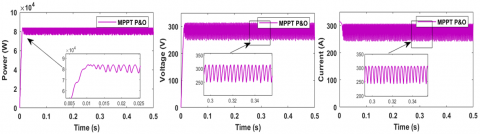
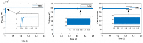
The Figures 11-14 present the systems response of power, voltage, and current of conventional method MPPT P&O and PI-GA, PI-PSO and PI-GWO respectively. It can be seen from Figure 11 that P&O MPPT control shows significant oscillations and persistent ripples, even during steady state across all three signals, i.e., Power, voltage and current. In addition, settling time is relatively slow. Indicating, an unstable tracking near MPP.
Figure 11. P&O MPPT output
Figure 12. PI-GA based controller output
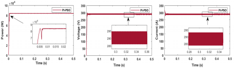
Figure 13. PI-PSO based controller output
Figure 14. PI-GWO based controller output
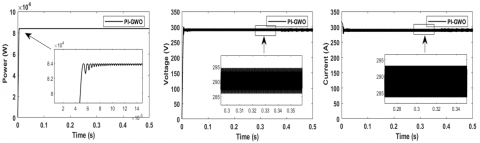
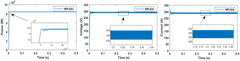
Figure 15. NPI-GA based controller
Figure 16. NPI-PSO based controller output
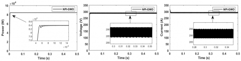
Figure 17. NPI-GWO based controller output
Figures 15-17 present the systems response of power, voltage, and current of the proposed non-linear controller NPI-GA, NPI-PSO and NPI-GWO respectively.
Table 7. Results of Non-linear NPI-based algorithms
|
Controller |
NPI-GA |
NPI-PSO |
NPI-GWO |
|
Overshoot (%) |
0.55 |
0.77 |
0.06 |
|
Rise time (s) |
0.004 |
0.004 |
0.004 |
|
Settling time (s) |
0.0047 |
0.0047 |
0.0048 |
|
Ripple (%) |
1.19 |
1.13 |
0.16 |
|
Efficiency (%) |
99.91 |
99.83 |
99.98 |
The implementation of nonlinear PI (NPI) controller showed improved performance compared to the conventional P&O MPPT and PI controller as it offers better energy efficiency, the nonlinear terms help accelerate convergence toward the MPP while reducing overshoot and oscillations. Combined with optimization algorithms, they reduced settling time, however, rise time remained the same. Analysis results are shown in the Table 7. Also, the use of NPI-GWO controller reduced the overvoltage and is very close to 289 (V), which is the MPP value under STC, whereas the other controllers delivered voltage close 295 (V). Finally, NPI-GWO controller also delivered the best performance overall and the highest efficiency of 99.98%.
6.2 Response of PV system at dynamic operating conditions
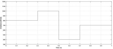
To evaluate the robustness and adaptability of the proposed control strategy, the system is tested under dynamic time varying irradiance in order to replicate realistic environmental conditions. This allows assessment of the controller’s tracking ability of MPP. Irradiance profile is presented in Figure 18, it ranges from 800 to 1000 to 400 to 700 W/m2.
Figure 19 illustrates the dynamic response of the PV system under varying irradiance conditions. To provide a more detailed analysis, three critical time intervals were selected and are shown with zoomed-in insets. These segments highlight the system’s behavior during initial transients, steady-state operation, and under sudden irradiance changes.
It can be shown from the zoom-in of segment (a) that the NPI-based controllers converge rapidly to the maximum power point with minimal overshoot and oscillations. In contrast, P&O MPPT shows more deviations and rise time is slow.
Segment (b): During steady state of the second segment, all methods experience some oscillations, but, NPI-GWO outperforms the other technique as it remains the closest to the MPP and has the lowest ripple amount and steady state error and then both NPI-GA and NPI-PSO shows good performance comparing it to PI-based MPPT and P&O MPPT.
Segment (c): Irradiance increase causes a sharp transition, yet, it is evident that NPI-GWO is the first to stabilize, quickly converging to the MPP with the smallest oscillations. Meanwhile, the PI-based controllers also track the MPP, but with more significant oscillations.
6.3 Statistically significant test
To perform the statistical significance analysis, controlled random noise was added to the irradiance input to evaluate the robustness of each controller and verify the reliability of the computed performance metrics. Each controller was tested over 20 simulation runs with different noise realizations, and the mean and standard deviation for each metric were calculated. Since the PI–GWO and NPI–GWO variants yielded the most competitive results, the statistical significance test was conducted on these two methods.
All p-values are below the 0.05 threshold, indicating that the performance differences between the PI–GWO and NPI–GWO controllers are statistically significant, as summarized in Table 8.
Table 8. Statistical significant analysis
|
Controller |
PI-GWO |
NPI-GWO |
p-Value |
|
Overshoot (%) |
1.22 ± 0.858 |
0.15±0.1 |
<0.05 |
|
Rise time (s) |
0.0042± 0.000037 |
0.0042± 0.000023 |
<0.05 |
|
Settling time (s) |
0.0051± 0.0025 |
0.0049± 0.000031 |
<0.05 |
|
Ripple (%) |
3.25± 0.15 |
0.16±0.003 |
<0.05 |
|
Efficiency (%) |
98.8±1.13 |
99.9±0.03 |
<0.05 |
In this study, the performance of advanced MPPT control strategies for a PV system was evaluated under both Standard Test Condition (STC) and dynamic operating conditions, in our case, varying irradiance levels. A nonlinear PI controller was implemented and optimized using three metaheuristic algorithms: PSO, GA, and GWO. Simulation results demonstrated that the use of nonlinear control significantly improved system performance compared to the conventional P&O method, particularly in terms of reduced overshoot, faster settling time, and minimized ripple, which is primarily due to the non-linear added gain. Among the tested methods, the NPI-GWO controller exhibited superior tracking accuracy, stability, and robustness.
These results highlight the need for a more robust control technique than conventional methods, as well as the use of more modern methods, such as artificial intelligence, to obtain more precise and calculated results, in this case optimal controller gains. In particular of non-linear PI controllers, which have more parameters than conventional PIs, making them more complicated to find. Future work could include experimental validation on real-time hardware, as well as extending the approach to grid-connected systems in partial shading.
|
MPP |
Maximum Power Point |
|
MPPT |
Maximum Power Point Tracking |
|
P&O |
Perturb and Observe |
|
InC |
Incremental Conductance |
|
PSO |
Particle Swarm Optimization |
|
GA |
Genetic Algorithm |
|
GWO |
Grey Wolf Optimization |
|
STC |
Standard Test Condition |
|
PID |
Proportional Intergal Derivative |
|
NPID |
Non-linear Proportional Integral Derivative |
|
PV |
Photovoltaic |
[1] Chala, G.T., Al Alshaikh, S.M. (2023). Solar photovoltaic energy as a promising enhanced share of clean energy sources in the future—A comprehensive review. Energies, 16(24): 7919. https://doi.org/10.3390/en16247919
[2] Sadeq, M.A., Abdulhadi, M.A., Talib, H.M. (2025). Advanced deep learning models for accurate solar energy output prediction. Journal Européen des Systèmes Automatisés, 58(3): 585-593. https://doi.org/10.18280/jesa.580315
[3] Annam, S., Srikrishna, S., Prabandhankam, S.R., Sivarajan, G. (2023). A prospective study on perturb observe MPPT methods for photovoltaic systems. Instrumentation, Mesure, Metrologie, 22(2): 73. https://doi.org/10.18280/jesa.570127
[4] Moulay, F., Habbati, A., Lousdad, A. (2022). The design and simulation of a photovoltaic system connected to the grid using a boost converter. Journal Européen des Systèmes Automatisés, 55(3): 367. https://doi.org/10.18280/jesa.550309
[5] Mauludin, M.S., Nugroho, A., Hidayat, A., Prasetyo, S.D. (2024). Simulation of AI-based PID controllers on DC machines using the matlab application. Journal Européen des Systèmes Automatisés, 57(1): 281-287. https://doi.org/10.18280/jesa.570127
[6] Abbas, I.A., Khamees, M. (2024). Automatic tuning of the PID controller based on the artificial gorilla troops optimizer. Iraqi Journal of Science, 65(5): 2867-2880. https://doi.org/10.24996/ijs.2024.65.5.40
[7] Joseph, S.B., Dada, E.G., Abidemi, A., Oyewola, D.O., Khammas, B.M. (2022). Metaheuristic algorithms for PID controller parameters tuning. Approaches and Open Problems. Heliyon, 8(5).
[8] Mazumdar, D., Sain, C., Biswas, P.K., Sanjeevikumar, P., Khan, B. (2024). Overview of solar photovoltaic MPPT methods: A state of the art on conventional and artificial intelligence control techniques. International Transactions on Electrical Energy Systems, 2024(1): 8363342. https://doi.org/10.1155/2024/8363342
[9] Ibrahim, A.W., Fang, Z., Li, R., Zhang, W., Xu, J., Zahir, V., ELrashidi, A. (2024). Intelligent nonlinear PID-controller combined with optimization algorithm for effective global maximum power point tracking of PV systems. IEEE Access, 12: 185265-185290. https://doi.org/10.1109/ACCESS.2024.3513355
[10] Aldulaimi, M.Y.M., Çevik, M. (2025). AI-enhanced MPPT control for grid-connected photovoltaic systems using ANFIS-PSO optimization. Electronics, 14(13): 2649. https://doi.org/10.3390/electronics14132649
[11] Malarvili, S., Mageshwari, S. (2022). Nonlinear PID (N-PID) controller for SSSP grid connected inverter control of photovoltaic systems. Electric Power Systems Research, 211: 108175. https://doi.org/10.1016/j.epsr.2022.108175
[12] Proaño, P., Pozo, M., Gallardo, C., Camacho, O. (2025). Non-linear PID control of AC current and DC voltage for a photovoltaic system operating on a microgrid. Results in Control and Optimization, 18: 100514. https://doi.org/10.1016/j.rico.2024.100514
[13] Thongpance, N., Chotikunnan, P., Wongkamhang, A., Chotikunnan, R., et al. (2025). Comparative analysis of PID tuning methods for speed control in Mecanum-wheel electric wheelchairs. Buletin Ilmiah Sarjana Teknik Elektro, 7(2): 95-110. https://doi.org/10.12928/biste.v7i2.13046
[14] Badis, A., Mansouri, M.N., Boujmil, M.H. (2019). Cascade control of grid‐connected PV systems using TLBO‐based fractional‐order PID. International Journal of Photoenergy, 2019(1): 4325648. https://doi.org/10.1155/2019/4325648
[15] Aripriharta, A., Syabani, M., Sendari, S., Wibawa, A.P., Susilo, S.W., Bagaskoro, M.C., Rosmin, N. (2025). MPPT performance analysis for PV energy harvesting using Grey Wolf Optimization (GWO) algorithm. ELKHA: Jurnal Teknik Elektro, 17(1): 68-76. https://doi.org/10.26418/elkha.v17i1.91643
[16] Khellaf, L., Djellal, A., Mayache, H., Sheta, A. (2024). Optimizing MPPT control of DC-DC boost converters using metaheuristic search algorithms and Nonlinear PID (N-PID) controllers. In International Conference on Artificial Intelligence in Renewable Energetic Systems, pp. 187-195. https://doi.org/10.1007/978-3-031-80301-7_21
[17] Djellal, A., Lakel, R. (2018). Adapted reference input to control PID-based active suspension system. Journal Européen des Systèmes Automatisés, 51(1-3): 7-23. https://doi.org/10.3166/JESA.51.7-23
[18] Eski, I., Yıldırım, Ş. (2009). Vibration control of vehicle active suspension system using a new robust neural network control system. Simulation Modelling Practice and Theory, 17(5): 778-793. https://doi.org/10.1016/j.simpat.2009.01.004
[19] Maddi, A., Guessoum, A., Berkani, D. (2014). Design of nonlinear PID controllers based on hyper-stability criteria. In 2014 15th International Conference on Sciences and Techniques of Automatic Control and Computer Engineering (STA), Hammamet, Tunisia, pp. 736-741. https://doi.org/10.1109/STA.2014.7086743
[20] Dobra, P., Truşcã, M. (2004). Robust stability of time-varying nonlinear systems using Popov criterion. IFAC Proceedings Volumes, 37(13): 1213-1216. https://doi.org/10.1016/S1474-6670(17)31392-7
[21] Salman, D., Elmi, Y.K., Isak, A.M., Sheikh-Muse, A. (2025). Evaluation of MPPT algorithms for solar PV systems with machine learning and metaheuristic techniques. Mathematical Modelling of Engineering Problems, 12(1): 115-124. https://doi.org/10.18280/mmep.120113
[22] Meddour, S., Rahem, D., Wira, P., Laib, H., Cherif, A. Y., Chtouki, I. (2022). Design and Implementation of an improved metaheuristic algorithm for maximum power point tracking algorithm based on a PV emulator and a double-stage grid-connected system. European Journal of Electrical Engineering/Revue Internationale de Génie Electrique, 24(3): 123-131. https://doi.org/10.18280/ejee.240301
[23] Nasir, M., Saloumi, M., Nassif, A.B. (2022). Review of various metaheuristics techniques for tuning parameters of PID/FOPID controllers. ITM Web of Conferences, 43: 01002. https://doi.org/10.1051/itmconf/20224301002
[24] El-Deen, A.T., Mahmoud, A.H., El-Sawi, A.R. (2015). Optimal PID tuning for DC motor speed controller based on genetic algorithm. International Review of Automatic Contraller, 8(1): 80-85. https://doi.org/10.15866/ireaco.v8i1.4839
[25] Irshad, A.S., Elkholy, M.H., Alshammari, N.F., Ludin, G.A., Senjyu, T., Pinter, G., Mikhaylov, A. (2024). Novel approach for energy balancing with intermittent renewable energy source using multi-objective genetic algorithm. IEEE Access, 12: 179318-179329. https://doi.org/10.1109/ACCESS.2024.3507216
[26] Sivaranjani, R., Rao, P.M. (2022). Smart energy optimization using new genetic algorithms in Smart Grids with the integration of renewable energy sources. Sustainable Networks in Smart Grid, pp. 121-147. https://doi.org/10.1016/B978-0-323-85626-3.00006-5
[27] Gomez, J., Chicaiza, W.D., Escano, J.M., Bordons, C. (2023). A renewable energy optimisation approach with production planning for a real industrial process: An application of genetic algorithms. Renewable Energy, 215: 118933. https://doi.org/10.1016/j.renene.2023.118933
[28] Harrag, A., Messalti, S. (2015). Variable step size modified P&O MPPT algorithm using GA-based hybrid offline/online PID controller. Renewable and Sustainable Energy Reviews, 49: 1247-1260. https://doi.org/10.1016/j.rser.2015.05.003
[29] Alakel, F., Kumar, S. (2024). GA and PSO techniques based optimal tuning of power system stabilizers in a PV integrated power network. European Journal of Engineering and Technology Research, 9(5): 1-7. http://doi.org/10.24018/ejeng.2024.9.5.3180
[30] Verdejo, H., Pino, V., Kliemann, W., Becker, C., Delpiano, J. (2020). Implementation of Particle Swarm Optimization (PSO) algorithm for tuning of power system stabilizers in multimachine electric power systems. Energies, 13(8): 2093. https://doi.org/10.3390/en13082093
[31] Jamhari, M.K.A.M., Hashim, N., Baharom, R., Othman, M.M. (2025). Simulation and verification of improved particle swarm optimization for maximum power point tracking in photovoltaic systems under dynamic environmental conditions. International Journal of Power Electronics and Drive Systems (IJPEDS), 16(1): 608-621. http://doi.org/10.11591/ijpeds.v16.i1
[32] Silaa, M.Y., Barambones, O., Bencherif, A., Rahmani, A. (2023). A new MPPT-based extended grey wolf optimizer for stand-alone PV system: A performance evaluation versus four smart MPPT techniques in diverse scenarios. Inventions, 8(6): 142. https://doi.org/10.3390/inventions8060142
[33] Zemmit, A., Loukriz, A., Belhouchet, K., Alharthi, Y.Z., Alshareef, M., Paramasivam, P., Ghoneim, S.S. (2025). GWO and WOA variable step MPPT algorithms-based PV system output power optimization. Scientific Reports, 15(1): 7810. https://doi.org/10.1038/s41598-025-89898-x
[34] Abdelmalek, F., Afghoul, H., Krim, F., Bajaj, M., Blazek, V. (2025). Experimental validation of novel hybrid grey Wolf equilibrium optimization for MPPT to improve the efficiency of solar photovoltaic system. Results in Engineering, 25: 103831. https://doi.org/10.1016/j.rineng.2024.103831
[35] Abdulhassan, S.K., Smida, M.B., Sakly, A., Tuaimah, F.M. (2025). Performance Comparison of FACTS (UPFC) and HVDC in power flow optimization via genetic algorithms. Journal Européen des Systèmes Automatisés, 58(3): 611. http://doi.org10.18280/jesa.580317
[36] Kennedy, J., Eberhart, R. (1995). Particle swarm optimization. In Proceedings of ICNN'95-International Conference on Neural Networks, Perth, WA, Australia, 4: 1942-1948. https://doi.org/10.1109/ICNN.1995.488968
[37] Kennedy, J. (2010). Particle swarm optimization. Anonymous encyclopedia of machine learning. In Proceedings of the Companion Publication of the 2014 Annual Conference on Genetic and Evolutionary Computation, Vancouver, BC, Canada, pp. 381-406. https://doi.org/10.1145/2598394.2605342
[38] Zermane, A.I., Bordjiba, T. (2024). Optimizing energy management of hybrid battery-supercapacitor energy storage system by using PSO-based fractional order controller for photovoltaic off-grid installation. Journal Européen des Systèmes Automatisés, 57(2): 465-475. https://doi.org/10.18280/jesa.570216
[39] Saady, I., Majout, B., Bossoufi, B., Karim, M., et al. (2025). Improving photovoltaic water pumping system performance with PSO-based MPPT and PSO-based direct torque control using real-time simulation. Scientific Reports, 15(1): 16127. https://doi.org/10.1038/s41598-025-00297-8
[40] Nanping, L., Kewen, X., Juan, Z., Chun, G. (2009). Numerical simulation on transistor with CQPSO algorithm. In 2009 4th IEEE Conference on Industrial Electronics and Applications, Xi'an, China, pp. 3732-3736. https://doi.org/10.1109/ICIEA.2009.5138900
[41] Mazumdar, D., Biswas, P. K., Sain, C., Ahmad, F., Al-Fagih, L. (2024). A comprehensive analysis of the optimal GWO based FOPID MPPT controller for grid-tied photovoltaics system under atmospheric uncertainty. Energy Reports, 12: 1921-1935. https://doi.org/10.1016/j.egyr.2024.08.013
[42] Chermite, C., Douiri, M.R. (2024). Enhancing photovoltaic cell parameters extraction through grey wolf optimizer. IFAC-PapersOnLine, 58(13): 624-629. https://doi.org/10.1016/j.ifacol.2024.07.552