Waleed Al-Ashtari![]()
© 2024 The author. This article is published by IIETA and is licensed under the CC BY 4.0 license (http://creativecommons.org/licenses/by/4.0/).
OPEN ACCESS
In this paper, the advantages of using adaptive controllers in active vehicle suspension systems to improve passenger comfort and safety are investigated. Based on Lyapunov analysis, the adaptation law of the controller is derived, where it uses the road profile and vehicle response to calculate the required control force. One of the advantages of the proposed controller is that it relies on a single tuning parameter, γ. In order to validate the proposed controller, MATLAB simulations are used to compare the performance of the proposed adaptively controlled system with that of both the uncontrolled and optimal controlled systems. The results show that the value of γ has significant effects on peak overshoot and the settling time of both vehicle displacement and acceleration. Furthermore, the results show a significant improvement between the adaptively controlled system and the uncontrolled system, with peak overshoot reductions of 44.6% and settling time reductions of 36%. The results also show that the adaptively controlled system proves its advantage by outperforming the optimal controlled system when dealing with large disturbances, but unfortunately, the adaptively controlled system typically requires a greater control force, twice as much as the optimal controlled system. Finally, the proposed adaptive controller exhibits remarkable performance and adaptability in responding effectively to changes in system parameters. This implies that, under many operational circumstances, it may be a trustworthy choice that ensures both the vehicle's safety and the comfort of its occupants.
adaptive control, vehicle suspension systems, LQR, Lyapunov theorem, fine-tuning parameter
A vehicle suspension system connects its body to its wheels using mechanical and electrical elements. The main responsibility of this system is to regulate how the tires interact with the road so that the car may be stable and safe while the occupants can ride comfortably [1].
These days, automobiles may have three basic kinds of suspension systems: active, semi-active, and passive. Every kind has its own approach to doing its job of enhancing the car's reaction to road conditions and providing comfort to its occupants [1-4].
The passive suspension mechanism is an old-fashioned one. It reduces the vibrations in automobiles through shock absorbers and springs, which have certain values. This kind of suspension system provides a basic degree of stability and comfort, but its performance may not be at its best under all driving circumstances [5].
A semi-active suspension system, on the other hand, consists of a rheological damper or another shock absorber with adjustable damping capacity. Typically, a controller included in a semi-active suspension system adjusts the shock absorber damping capacity to ensure safe and enjoyable riding. Semi-active systems lack the power of active systems, even if they are more flexible than passive ones [6, 7].
The most complex suspension systems are active. By using controllers, electronic sensors, and actuators, these suspension systems actively manage how the car reacts to road irregularities using comptroller, electronic sensors, and actuators. Usually, to alter the performance of the car, the controller manages the force magnitude of the actuator to alter the car's efficiency. This implies that the car's dynamics change depending on road conditions and the vehicle's status. This kind of suspension can work correctly even in cases where mechanical factors like stress and fatigue alter the suspension characteristics. They may successfully compensate for road imperfections and preserve correct operation [8-11].
Suspension systems generally use control algorithms to enhance ride comfort, stability, and safety. These algorithms use sensor data to calculate the appropriate suspension system modification. This modification can affect either the force the actuator delivers in an active system or the damping capacity in a semi-active system, as previously mentioned. Optimal and adaptive control algorithms are the two basic categories of controllers. Optimal control aims to optimize the controller parameters for a specific performance by taking into account system dynamics and disturbances. On the other hand, adaptive control measures system dynamics and disturbances and uses them as inputs to the adaptation law to repeatedly update the controller parameters [12].
There are still many obstacles to overcome and chances for improvement, even if the area of adaptive control for active suspension systems has advanced significantly. In order to further current understanding, this work presents an adaptive controller based on state feedback control that dynamically modifies the suspension system's reaction to road circumstances. Adaptive control in active car suspension systems has been the subject of many published techniques and approaches to achieve consistent suspension system performance at various road imperfections. Proportional-integral-derivative (PID), sliding mode control (SMC), and fuzzy logic control (FLC) are among the numerous control strategies previously studied. Each of these approaches has pros and cons of its own.
PID controls are simple to implement in suspension systems to improve their performance and stability. However, implementing PID control in suspension systems presents numerous challenges, including gain tuning and nonlinearities. Usually, adaptive control approaches adjust the PID controller's gains based on specific adaptation rules that consider the vehicle's condition [13-18].
On the other hand, using sliding mode control (SMC) in suspension systems provides reliable functioning in the face of uncertainties and disturbances. By creating a stable sliding surface, the controller ensures effective responses to various traffic scenarios. This approach greatly enhances both vehicle control and safety, but unfortunately, chatting with SMC might have a negative effect on ride comfort [19-30].
Alternately, fuzzy logic controllers (FLCs) find use in automotive suspension systems [31-39]. Moreover, a number of research publications integrate FLCs with SMCs or PID controllers. This is because FLCs can improve the performance of these controllers in complex and uncertain situations by resolving their shortcomings. FLCs provide these controllers with extra robustness and effectively address nonlinearities [40-57].
Many published works use inertial profilers, or LIDAR, to detect road imperfections. Recently, there has been a trend to use the suspension response itself as an input for the controller, utilizing onboard sensors such as accelerometers and potentiometers [58-64].
This work attempts to further develop the adaptive control of active suspension systems by presenting a novel adaptive controller that operates depending on the measurement of both road profile and suspension response. The adaptation mechanism of the proposed controller will be derived based on Lyapunov's stability analysis. An optimal controller (LQR) for the suspension system will be introduced in order to validate the proposed adaptive controller. Also, MATLAB will be used to simulate and analyze the proposed adaptively controlled, optimally controlled, and uncontrolled suspension systems. All three systems will be assessed for their performance across various road profiles and system uncertainties. At the end, the results, limitations, and capabilities of the proposed controller will be reviewed.
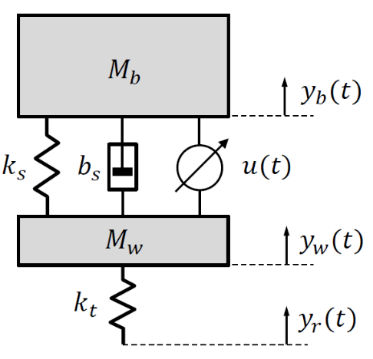
In vehicle engineering, a quarter-car model is a shortened approximation that studies the dynamic behavior of a suspension system. This study uses the controlled quarter-car model, as illustrated in Figure 1. Within this model, the control force is represented by u(t), the vehicle body displacement by yb(t), the wheel displacement by yw(t), and the road profile by yr(t).
Figure 1. Illustration diagram of the controlled suspension system
Using Newton's second law, the governing equations of the vehicle body can be expressed as:
$\begin{array}{r}M_b \ddot{y}_b(t)+b_s\left(\dot{y}_b(t)-\dot{y}_w(t)\right)+k_s\left(y_b(t)-\right. \left.y_w(t)\right)=u(t)\end{array}$ (1)
and, for the wheel, it can be written as:
$\begin{gathered}M_w \ddot{y}_w(t)+b_s\left(\dot{y}_w(t)-\dot{y}_b(t)\right)+k_s\left(y_w(t)-\right. \left.y_b(t)\right)+k_t\left(y_w(t)-y_r(t)\right)=-u(t)\end{gathered}$ (2)
where, the masses of the body of the vehicle and its wheels are denoted by Mb and Mw, respectively. Moreover, the damping coefficient of the suspension system is denoted by bs; the stiffness of the suspension and the tire are denoted by ks and kt.
Assuming x1(t)=yb(t), $x_2(t)=\dot{y}_b(t)$, x3(t)=yw(t), and $x_4(t)=\dot{y}_w(t)$, then substituting these into Eq. (1) and Eq. (2) gives:
$\begin{gathered}\dot{x}_2(t)=-\frac{k_s}{M_b} x_1(t)-\frac{b_s}{M_b} x_2(t)+\frac{k_s}{M_b} x_3(t)+ \frac{b_s}{M_b} x_4(t)+\frac{1}{M_b} u(t)\end{gathered}$ (3)
and
$\begin{aligned} \dot{x}_4(t)= & \frac{k_s}{M_w} x_1(t)+\frac{b_s}{M_w} x_2(t)-\left(\frac{k_t+k_s}{M_w}\right) x_3(t)-\frac{b_s}{M_w} x_4(t)-\frac{1}{M_w} u(t)+\frac{k_t}{M_w} y_r(t)\end{aligned}$ (4)
Now, rewriting the differential equations presented in Eq. (3) and Eq. (4) in matrix form, such as:
$\begin{aligned} & {\left[\begin{array}{l}\dot{x}_1(t) \\ \dot{x}_2(t) \\ \dot{x}_3(t) \\ \dot{x}_4(t)\end{array}\right]=} {\left[\begin{array}{cccc}0 & 1 & 0 & 0 \\ -\frac{k_s}{M_b} & -\frac{b_s}{M_b} & \frac{k_s}{M_b} & \frac{b_s}{M_b} \\ 0 & 0 & 0 & 1 \\ \frac{k_s}{M_w} & \frac{b_s}{M_w} & -\left(\frac{k_t+k_s}{M_w}\right) & -\frac{b_s}{M_w}\end{array}\right]\left[\begin{array}{l}x_1(t) \\ x_2(t) \\ x_3(t) \\ x_4(t)\end{array}\right]+} {\left[\begin{array}{c}0 \\ \frac{1}{M_b} \\ 0 \\ -\frac{1}{M_w}\end{array}\right] u(t)+\left[\begin{array}{c}0 \\ 0 \\ 0 \\ \frac{k_t}{M_w}\end{array}\right] y_r(t)} \\ & \end{aligned}$ (5)
and
$\left[\begin{array}{l}y_1(t) \\ y_2(t) \\ y_3(t) \\ y_4(t)\end{array}\right]=\left[\begin{array}{llll}1 & 0 & 0 & 0 \\ 0 & 1 & 0 & 0 \\ 0 & 0 & 1 & 0 \\ 0 & 0 & 0 & 1\end{array}\right]\left[\begin{array}{l}x_1(t) \\ x_2(t) \\ x_3(t) \\ x_4(t)\end{array}\right]$ (6)
As a result, the state space model for the suspension system provided in Eq. (5) can be written as:
$\dot{x}(t)=A x(t)+B u(t)+W y_r(t)$ (7)
where, x(t) represents the state variable of the system, and y(t) is the output state, which may be stated as:
$y(t)=C x(t)$ (8)
Given here is the system matrix A:
$A=\left[\begin{array}{cccc}0 & 1 & 0 & 0 \\ -\frac{k_s}{M_b} & -\frac{b_s}{M_b} & \frac{k_s}{M_b} & \frac{b_s}{M_b} \\ 0 & 0 & 0 & 1 \\ \frac{k_s}{M_w} & \frac{b_s}{M_w} & -\left(\frac{k_t+k_s}{M_w}\right) & -\frac{b_s}{M_w}\end{array}\right]$ (9)
One may state the input matrix B as:
$B=\left[\begin{array}{llll}0 & \frac{1}{M_b} & 0 & -\frac{1}{M_w}\end{array}\right]^T$ (10)
The reference matrix W can be written as:
$W=\left[\begin{array}{llll}0 & 0 & 0 & \frac{k_t}{M_w}\end{array}\right]^T$ (11)
At last, one may depict the output matrix C as:
$C=\left[\begin{array}{llll}1 & 0 & 0 & 0 \\ 0 & 1 & 0 & 0 \\ 0 & 0 & 1 & 0 \\ 0 & 0 & 0 & 1\end{array}\right]$ (12)
These matrices will be very important for the next parts that create the proposed adaptive controller. They will be used in MATLAB to model the optimal controller as well. The performance of the proposed controller is to be assessed using this simulation.
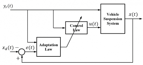
Figure 2. Functional block diagram of the proposed adaptive controller
The functional block diagram shown in Figure 2 illustrates the proposed controller's configuration. The control process begins by measuring the vehicle states x(t) and comparing them with the desired states xd(t) in order to calculate the error signal e(t) that is used with the measured road profile yr(t) to deduce the required controller parameters based on the derived adaptation law. These parameters will then be used by the proposed control law to compute the control force u(t) that will work quickly to bring the vehicle states x(t) into the desired states xd(t). This control process is repeated continuously during motion to improve passenger comfort.
The error e(t) is assumed to be:
$e(t)=x(t)-x_d(t)$ (13)
In suspension system applications, the desired state xd(t) of the vehicle is assumed to be zero to prioritize passenger comfort. Consequently, Eq. (13) can be expressed as:
$e(t)=x(t)$ (14)
Therefore, the error rate of change $\dot{e}(t)$ can be expressed as:
$\dot{e}(t)=\dot{x}(t)$ (15)
Substituting Eq. (7) into Eq. (15) yields:
$\dot{e}(t)=A x(t)+B u(t)+W y_x(t)$ (16)
Applying state feedback control theory, the control law can be expressed as:
$u(t)=-k_x y_r(t)$ (17)
where, kr represents the controller gain. Substituting Eq. (17) into Eq. (16) results in the following expression:
$\dot{e}(t)=A x(t)+\left(W-B k_r\right) y_r(t)$ (18)
Eq. (18) illustrates the relationship between the system states, errors rate, and design factors. It stated that when this relationship, W=Bkr, is correct, there will be a direct connection between the states x(t) and the errors rate $\dot{e}(t)$. This implies that as the states x(t) approach zero, so do the errors rate $\dot{e}(t)$. Thus, the control law will be proposed based on this finding.
In practical applications, wear, deformation, and friction may cause system parameters A and B to change over time. As a result, the gain kr is difficult to accurately calculate. To overcome this difficulty, the control law is rewritten as follows:
$u(t)=-\hat{k}_r y_x(t)$ (19)
where, $\hat{k}_r(t)$ is the estimation of the gain kr. Now, substituting Eq. (19) into Eq. (16), which gives:
$\dot{e}(t)=A x(t)+\left(W-B \hat{k}_r\right) y_r(t)$ (20)
It can be noted that the estimation gain $\hat{k}_r(t)$ is varying with time, and they assumed to be expressed as:
$\tilde{k}_r(t)=k_r-\hat{k}_r(t)$ (21)
where, $\tilde{k}_r(t)$ is the error in estimating the gain kr. Substituting Eq. (21) into Eq. (20) gives:
$\dot{e}(t)=A x(t)+\left(W-B k_r+B \tilde{k}_r(t)\right) y_r(t)$ (22)
By plugging in the outcomes of Eq. (18) and Eq. (19) into Eq. (22) and making a few math simplifications, the expression transforms into:
$\dot{e}(t)=B \tilde{k}_r(t) y_r(t)$ (23)
Now, Lyapunov stability analysis will be used to derive the adaptation law for the proposed controller. It begins by defining a suitable Lyapunov function, V(t), which leads to having the adaptation law that ensures the stability of the closed-loop system. The Lyapunov function is chosen such that its time derivative along the trajectories of the closed-loop system is negative semi-definite. Thus, the following candidate function can be proposed:
$V(t)=\frac{1}{2} e^2(t)+\frac{1}{2} \widetilde{k}_r^2(t)$ (24)
The time derivative of the Lyapunov function can be written as:
$\dot{V}(t)=e(t) \dot{e}(t)+\tilde{k}_r(t) \dot{\tilde{k}}_r(t)$ (25)
The time derivatives of $\tilde{k}_r(t)$ can be written as:
$\dot{\tilde{k}}_r(t)=-\dot{\hat{k}}_r(t)$ (26)
Substituting Eq. (26), and Eq. (23) into Eq. (25), which leads to:
$\dot{V}(t)=B y_r(t) e(t) \tilde{k}_r(t)-\dot{\hat{k}}_r \tilde{k}_r(t)$ (27)
According to Lyapunov's direct method, stability of the system can be guaranteed if $\dot{V}(t)$ goes to zero as time tends to infinity. Therefore, the following relationship should be provided:
$\dot{\hat{k}}_r(t)=B y_r(t) e(t)$ (28)
Substituting Eq. (10) and Eq. (14) into Eq. (28) and making a few mathematical simplifications yields:
$\dot{\hat{k}}_r(t)=\gamma y_r(t) x(t)$ (29)
In this context, γ represents a constant. As γ is a positive definite constant, it ensures that $\dot{V}(t)$ is zero, thereby ensuring the stability of the closed-loop system. Adjusting γ allows for fine-tuning of the controller's performance to align with the designer's preferences.
This section, Introducing the Linear Quadratic Regulator (LQR) Optimal Controller, aims to examine how well the proposed adaptive controller works and what its features are. LQR is defined as a robust controller extensively used in designing feedback control systems for linear dynamic systems. It provides optimal performance and stability assurances. Due to its versatility, this controller finds widespread use across a variety of real-life applications [65].
To ensure precise regulation and tracking, it is assumed that the optimal controller's control law can be written as:
$u_{o p}(t)=-k_1 x(t)-k_2 y_r(t)$ (30)
where, uop(t) is the optimal control force. Furthemore, k1 and k2 are optimal gain vectors. The essence of LQR control lies in seeking the optimal control action to efficiently stabilize the system. This goal is attained by minimizing a performance index termed J, represented as:
$J=\int_0^{\infty}\left(x(t)^T Q x(t)+u_{o p}^T R u_{o p}\right) d t$ (31)
where, Q is a positive semidefinite weighting matrix for the state variables x(t), and R is a positive definite weighting matrix for the control input uop(t). The goal of the LQR controller is to minimize this cost function by calculating selecting the control input uop(t) based on the state x(t) of the system. In this paper, the MATLAB Command ‘lqr’ will be used to calculate the gain vectors k1 and k2 based on inputting proper Q and R depending on the desirable suspension system performance.
In this part, the performance of the proposed controller will be validated under actual circumstances and its potential for practical applications will be explored via a thorough case study. We will run the simulation using MATLAB, a well-known dynamic system analysis software. In Table 1, the particular parameters used in the case study are described.
Table 1. Specifications of the employed suspension system parameters
|
Description |
Symbol |
Unit |
Value |
|
Body mass |
Mb |
kg |
300 |
|
Wheel mass |
Mw |
kg |
60 |
|
Suspension stiffness |
ks |
N/m |
16000 |
|
Suspension damping coefficient |
bs |
N⋅s/m |
1000 |
|
Tier stiffness |
kt |
N/m |
190000 |
The road profile encompasses two distinct bumps and is defined by the following equation:
$y_r(t)=\left\{\begin{array}{cc}\delta_1(1-\cos 4 \pi t), & 0 \leq t \leq 0.5 \\ \delta_2(1-\cos 4 \pi t), & 2 \leq t \leq 2.5 \\ 0, & \text { otherwise }\end{array}\right.$ (32)
The investigation will consider two road profiles based on the values of the constants δ1 and δ2. In the first road profile, δ1 is set to 0.02 m and δ2 is set to 0.03 m. In the second road profile, the constants are interchanged, making δ1 equal to 0.03 m and δ2 equal to 0.02 m. This setup facilitates the examination of the suspension system's response to varying levels of disturbance. In the first profile, the suspension system will encounter a smaller disturbance initially, followed by a larger disturbance. Conversely, in the second profile, the suspension system will face a larger disturbance followed by a smaller one. The investigation aims to demonstrate the robustness of the controller under different conditions, highlighting its ability to adapt to varying road profiles.
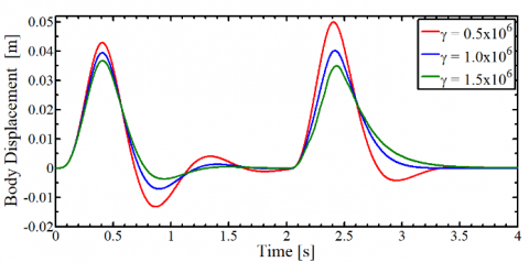
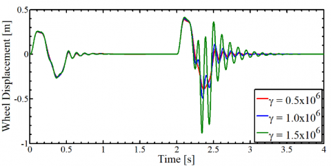
Analysis of Eq. (29) reveals the significant impact of the tuning parameter γ on the suspension system's response. Consequently, an initial simulation is conducted with varying values of γ to ascertain the optimal parameter. Figures 3 and 4 illustrate the displacements of both the vehicle body and the wheel resulting from applying the first road profile. These figures distinctly demonstrate that augmenting the tuning parameter γ enhances the suspension response, thereby ensuring passenger comfort.
Figure 3. Body displacement at different values of the tuning parameter γ
Figure 4. Wheel displacement at different values of the tuning parameter γ
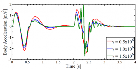
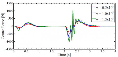
To determine the most suitable tuning parameter γ, further data concerning body acceleration and the corresponding control force for each γ value is essential. Figures 5 and 6 illustrate the body acceleration and control force, respectively. Minimizing body acceleration is crucial for passenger comfort, while keeping the control force at a reasonable and minimal level is paramount to avoid discomfort. After thorough deliberation, a value of γ=1×10⁶ is selected. This choice results in an exemplary response with minimal exertion compared to alternative cases, aligning closely with the preferences of the designers. The chosen value of the tuning parameter γ will now be implemented in the subsequent analysis. Furthermore, the investigation expanded to include the optimal controlled system, where various Q and R matrices were employed as inputs in the system simulation. Through meticulous analysis of the results, it was determined that the most effective matrices were a unity matrix of 4×4 dimensions for Q and R=1×10⁻⁶[1 1]T. This careful selection of matrices not only underscores the depth of the research but also highlights the precision in optimizing the system's performance.
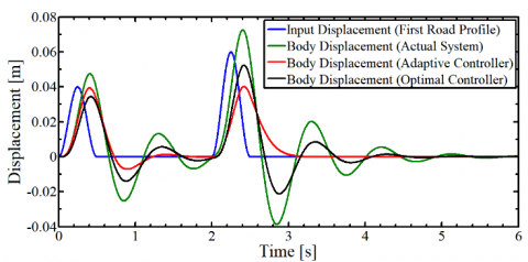
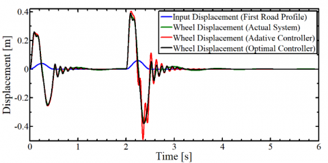
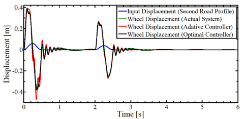
In Figures 7a and 7b, the input displacements (road profiles) are compared with the corresponding body displacements of the actual suspension system, the suspension system equipped with the proposed adaptive control, and the suspension system equipped with an optimal control.
Figure 5. Body acceleration at different values of the tuning parameter γ
Figure 6. Control force at different values of the tuning parameter γ
(a) Body displacements under first road profile
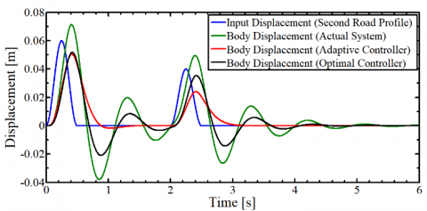
(b) Body displacements under second road profile
Figure 7. Body displacements of the investigated systems under different road profiles
In Figure 7a, significant enhancements are observed for both controlled systems. The figure demonstrates that for the initial bump, the actual system fails to reach a stable state. The adaptive controlled system reduces peak overshoot by 17%, with a markedly improved settling time of 1.56 seconds (considering a 2% criterion). In contrast, the optimal controlled system reduces peak overshoot by 37% and never reaches 2% of its value. For the second bump, the adaptive controlled system exhibits a substantial 44.6% reduction in peak overshoot and settles in approximately 3.2 seconds, compared to the optimal controlled system which achieves a 27.3% reduction in peak overshoot and settles in approximately 4.4 seconds. The adaptive controller appears more effective than the others at mitigating fast or large road disturbances.
In Figure 7b, significant enhancements are again evident for both controlled systems. For the initial bump, the actual system fails to reach a stable state. Both the adaptive and optimal controlled systems achieve a similar reduction in peak overshoot, approximately 27%, while the settling time of the adaptive controlled system is notably shorter at 1.21 seconds, compared to the optimal and actual systems which never settle. For the second bump, the adaptive controlled system demonstrates a substantial 51.5% reduction in peak overshoot and settles in approximately 3.0 seconds, whereas the optimal controlled system achieves a 28.5% reduction in peak overshoot and settles in approximately 4.4 seconds. The actual system has a settling time of about 4.8 seconds. These results confirm the effectiveness of the proposed adaptive controller, particularly under adverse road conditions.
Furthermore, Figures 8a and 8b demonstrate minimal disparity between the different investigated systems under the two types of road profiles, except at the peak of the larger bump. Here, the wheel displacement of the adaptively controlled system experiences a 32% increase, strategically implemented to counteract the bump's effect on the vehicle body. This refined approach showcases significant advancements in the system's overall performance and robustness.
(a) Wheel displacements under First road profile
(b) Wheel displacements under second road profile
Figure 8. Wheel displacements of the investigated systems under different road profiles
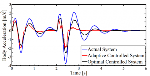
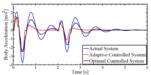
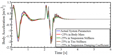
As previously emphasized, the acceleration of the vehicle body holds paramount importance in ensuring passenger comfort. Figures 9a and 9b provide comprehensive comparisons, each displaying three distinct curves illustrating the acceleration profiles of the actual system, the adaptive controlled system, and the optimal controlled system under one of the utilized road profiles. A discernible difference is immediately evident. The adaptive controlled system excels in terms of settling time and peak overshoot, showcasing a remarkable 46% reduction in maximum acceleration. This compelling improvement underscores the enhanced comfort and stability achieved through the proposed adaptive control methodology.
(a) Body acceleration under first road profile
(b) Body acceleration under second road profile
Figure 9. Body accelerations of the investigated systems under different road profiles
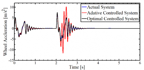
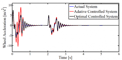
Additionally, an examination of wheel acceleration provides a holistic perspective on the performance of the three investigated systems. Illustrated in each of Figures 10 are three distinct curves representing the acceleration profiles of the wheel under one of the utilized road profiles. It is evident that the adaptive controlled system registers higher levels of acceleration in the wheel; at certain moments, it reaches levels twice those of the actual system and the optimal controlled system. This discrepancy underscores the adeptness with which the controlled system manages the energy input from the road profile. By directing a substantial portion of this energy towards the wheel, the controlled system prioritizes passenger comfort and safeguards the integrity of the vehicle body. This nuanced approach, coupled with meticulously designed wheel and associated parameters, lays the foundation for a dependable suspension system that significantly enhances passenger comfort.
(a) Wheel acceleration under first road profile
(b) Wheel acceleration under second road profile
Figure 10. Wheel accelerations of the investigated systems under different road profiles
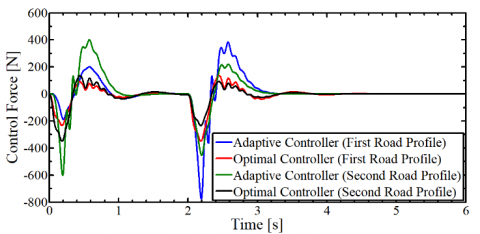
Figure 11 demonstrates the optimal controller's superiority over the adaptive controller in determining the required control force for different road profiles. In certain situations, the adaptively controlled system necessitates a control force that is 2.2 times greater than the optimally controlled system. However, this figure also shows the superiority of the adaptive controller in dealing with large disturbances. This occurs because the adaptive controller relies directly on system states and road profile data for its calculations, which prioritize passenger comfort over the magnitude of the control force. Overall, it is critical to carefully design suspension system elements and choose the tuning parameter γ to maximize performance.
Figure 11. Comparison of required control force for adaptive and optimal controllers under different road profiles
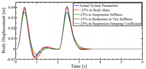
Figure 12. Comparing body displacements: Adaptive controlled vs. actual suspension systems with varying parameters and identical input excitation
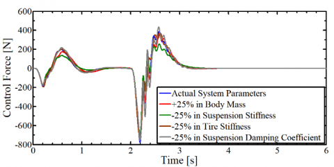
In practical applications, variations in important factors such as body mass, suspension stiffness, damping coefficient, and tire stiffness cause problems for suspension systems. Mechanical wear or changing loading conditions over time can cause these differences. Figures 12, 13, and 14 demonstrate the assessment of the proposed adaptively controlled suspension system under various parameter modifications. These figures show how effectively the system performs under changing conditions, as well as how flexible and resilient it is to anticipated interruptions in the suspension system's functioning. Crucially, even when suspension characteristics vary, passenger comfort metrics like body displacement and acceleration, as well as vehicle safety factors like control force, are mostly constant. Every instance examined has a consistent settling time.
Figure 13. Comparing wheel displacements: Controlled vs. actual suspension systems with varying parameters and identical input excitation
Figure 14. Control force variation with changing suspension system parameters
The performance of the adaptively controlled suspension systems is significantly influenced by the tuning parameter γ. Based on extensive simulation testing, it is clear that a value of 106 produces the optimal results.
In terms of performance, the adaptively controlled system proves to be better than both the actual system and the optimal controlled system, particularly when dealing with large disturbances. During large disturbances, the adaptation law allows for an overestimation of the control force, ensuring rapid suppression of body displacement and passenger comfort. Therefore, the system requires a larger control force, typically twice that of an optimal controller. In the meantime, the wheel acceleration for the adaptively controlled system is also twice that of an optimal controller.
The main benefit of using the proposed adaptive controller is the noticeable decrease in both displacement and acceleration of the vehicle's body. The results demonstrate a remarkable 44.6% reduction in peak overshoot of body displacement, accompanied by a 36% reduction in settling time and a 46% reduction in body acceleration. Thus, these results show how the adaptively controlled system provides a more comfortable and safer ride for the vehicle and the passengers, surpassing the performance of the actual system.
Additionally, the findings show that the adaptively controlled suspension system responds well to changes in system parameters. The adaptation law replaces the effects of changing parameters with the control force, which keeps the body's displacement and acceleration almost constant.
In closing, the well-selected tuning parameter γ has enabled the adaptively controlled suspension system to exhibit optimal performance, characterized by improvements in ride comfort and safety. Therefore, future investigations may focus primarily on optimizing this parameter.
The authors would like to thank all the staff of the Mechanical Engineering Department, College of Engineering, University of Baghdad, for their support and assistance.
|
A |
system matrix |
|
B |
input matrix |
|
C |
output matrix |
|
bs |
damping coefficient of the suspension, N. s. m-1 |
|
e(t) |
error represents x(t)-xd(t) |
|
J |
performance index of the optimal controller |
|
k1 |
optimal gain vector of x(t) |
|
k2 |
optimal gain vector of yr(t) |
|
kr |
controller gain, N. m-1 |
|
$\hat{k}_r(t)$ |
estimation of the gain kr, N. m-1 |
|
$\tilde{k}_r(t)$ |
error in estimating the gain kr, N. m-1 |
|
ks |
stiffness of the suspension, N. m-1 |
|
kt |
stiffness of the tire, N. m-1 |
|
Mb |
masses of the vehicle body, Kg |
|
Mw |
masses of the vehicle wheel, Kg |
|
Q |
positive semidefinite weighting matrix for the state variables x(t) |
|
R |
positive definite weighting matrix for the control input uop(t) |
|
u(t) |
control force, N |
|
uop(t) |
optimal control force, N |
|
V(t) |
Lyapunov function |
|
W |
reference matrix |
|
x(t) |
state space of the system |
|
xd(t) |
desired state of the system |
|
x1(t) |
state space variable represents yb(t), m |
|
x2(t) |
state space variable represents $\dot{y}_b(t)$, m.s-1 |
|
x3(t) |
state space variable represents yw(t), m |
|
x4(t) |
state space variable represents $\dot{y}_w(t)$, m.s-1 |
|
y(t) |
state space output |
|
yb(t) |
displacement of the vehicle body, m |
|
yr(t) |
input displacement (road profile), m |
|
yw(t) |
displacement of the vehicle wheel, m |
|
y1(t) |
state space output represents x1(t), m |
|
y2(t) |
state space output represents x2(t), m.s-1 |
|
y3(t) |
state space output represents x3(t), m |
|
y4(t) |
state space output represents x4(t), m.s-1 |
|
Greek symbols |
|
|
γ |
fine-tuning parameter of the controller |
|
δ1 |
constant for defining the road profile, m |
|
δ2 |
constant for defining the road profile, m |
|
Subscripts |
|
|
FLC |
Fuzzy Logic Control |
|
LQR |
Linear Quadratic Regulator |
|
PID |
Proportional-Integral-Derivative |
|
SMC |
Sliding Mode Control |
[1] Goodarzi, A., Lu, Y., Khajepour, A. (2023). Vehicle suspension system technology and design. Springer Nature. http://doi.org/10.1007/978-3-031-21804-0
[2] Kashem, S., Nagarajah, R., Ektesabi, M. (2018). Vehicle suspension systems and electromagnetic dampers. Springer Tracts in Mechanical Engineering. http://doi.org/10.1007/978-981-10-5478-5
[3] Jiregna, I., Sirata, G. (2020). A review of the vehicle suspension system. Journal of Mechanical and Energy Engineering, 4(2): 109-114. http://doi.org/10.30464/jmee.2020.4.2.109
[4] Llopis-Albert, C., Francisco, R., Shouzhen, Z. (2023). Multiobjective optimization framework for designing a vehicle suspension system. A comparison of optimization algorithms. Advances in Engineering Software, 176: 103375. http://doi.org/10.1016/j.advengsoft.2022.103375
[5] Shelke, D., Anirban, C., Vinay, R. (2018). Validation of simulation and analytical model of nonlinear passive vehicle suspension system for quarter car. Materials Today: Proceedings, 5(9): 19294-19302. http://doi.org/10.1016/j.matpr.2018.06.288
[6] Aladdin, M. F., Singh, J. (2018). Modelling and simulation of semi-active suspension system for passenger vehicle. Journal of Engineering Science and Technology, 7: 104-107.
[7] Walavalkar, S., Tandel, V., Thakur, R.S., Kumar, V.P., Bhuran, S. (2021). Performance comparison of various controllers on semi-active vehicle suspension system. ITM Web of Conferences, 40: 01001. http://doi.org/10.1051/itmconf/20214001001
[8] Kumar, S., Amit, M., Raghuvir, K. (2021). Modeling of an active suspension system with different suspension parameters for full vehicle. Indian Journal of Engineering and Materials Sciences, 28(1): 55-63. http://doi.org/10.56042/ijems.v28i1.31353
[9] Sibielak, M., Waldemar, R., Jaroslaw, K. (2019). Modelling and control of a full vehicle active suspension system. In 20th International Carpathian Control Conference (ICCC), pp. 1-6. http://doi.org/10.1109/CarpathianCC.2019.8766004
[10] Rezanoori, A., Ariffin, M., Delgoshaei, A., Jalil, N., Zulkefli, Z. (2019). A new method to improve passenger vehicle safety using intelligent functions in active suspension system. Engineering Solid Mechanics, 7(4): 313-330. http://doi.org/10.5267/j.esm.2019.6.005
[11] Papagiannis, D., Evangelos, T., Markos, K., Nikolaos, J., Christos, M. (2021). Enhancing the braking performance of a vehicle through the proper control of the active suspension system. IEEE Access, 9: 155936-155948. http://doi.org/10.1109/ACCESS.2021.3129263
[12] Jing, D., Sun, J.Q., Ren, C.B., Zhang, X.H. (2020). Multi-objective optimization of active vehicle suspension system control. In Nonlinear Dynamics and Control: Proceedings of the First International Nonlinear Dynamics Conference (NODYCON 2019), pp. 137-145. http://doi.org/10.1007/978-3-030-34747-5_14
[13] Huang, D.S., Zhang, J.Q., Liu, Y.L. (2018). The PID semi-active vibration control on nonlinear suspension system with time delay. International Journal of Intelligent Transportation Systems Research, 16(2): 125-137. http://doi.org/10.1007/s13177-017-0143-5
[14] Altinoz, O., Egemen, A. (2018). Optimal PID design for control of active car suspension system. International Journal of Information Technology and Computer Science (IJITCS), 10(1): 16-23. http://doi.org/10.5815/ijitcs.2018.01.02
[15] Pillai, S., Chithirai, P., Sahith, R. (2019). Design of PID control to improve efficiency of suspension system in electric vehicles. In 2019 International Conference on Computational Intelligence and Knowledge Economy (ICCIKE), pp. 570-575. http://doi.org/10.1109/ICCIKE47802.2019.9004322
[16] Huang, J. (2020). Suspension system based on PID control. In Innovative Computing: IC 2020, pp. 101-106. http://doi.org/10.1007/978-981-15-5959-4_12
[17] Tian, M., Vanliem, N. (2020). Control performance of suspension system of cars with PID control based on 3D dynamic model. Journal of Mechanical Engineering, Automation and Control Systems, 1(1): 1-10. http://doi.org/10.21595/jmeacs.2020.21363
[18] Shafiei, B. (2022). A review on PID control system simulation of the active suspension system of a quarter car model while hitting road bumps. Journal of the Institution of Engineers (India): Series C, 103(4): 1001-1011. http://doi.org/10.1007/s40032-022-00821-z
[19] Chen, S.A., Wang, J.C., Yao, M., Kim, Y.B. (2017). Improved optimal sliding mode control for a non-linear vehicle active suspension system. Journal of Sound and Vibration, 395: 1-25. http://doi.org/10.1016/j.jsv.2017.02.017
[20] Ozer, H., Hacioglu, Y., Yagiz, N. (2018). High order sliding mode control with estimation for vehicle active suspensions. Transactions of the Institute of Measurement and Control, 40(5): 1457-1470. https://doi.org/10.1177/0142331216685394
[21] Bai, R., Guo, D. (2018). Sliding-mode control of the active suspension system with the dynamics of a hydraulic actuator. Complexity, 2018: 5907208. https://doi.org/10.1155/2018/5907208
[22] Wang, D., Zhao, D., Gong, M., Yang, B. (2018). Nonlinear predictive sliding mode control for active suspension system. Shock and Vibration, 2018: 8194305. https://doi.org/10.1155/2018/8194305
[23] Abtahi, S.M. (2019). Suppression of chaotic vibrations in suspension system of vehicle dynamics using chattering-free optimal sliding mode control. Journal of the Brazilian Society of Mechanical Sciences and Engineering, 41(5): 210. https://doi.org/10.1007/s40430-019-1711-1
[24] Rui, B. (2019). Nonlinear adaptive sliding-mode control of the electronically controlled air suspension system. International Journal of Advanced Robotic Systems, 16(5): 1729881419881527. http://doi.org/10.1177/1729881419881527
[25] Al-Samarraie, S., Hama, T. (2019). Robust adaptive sliding mode controller for a nonholonomic mobile platform. Journal of Engineering, 25(8): 19-38. http://doi.org/10.31026/j.eng.2019.08.02
[26] Qin, W., Shangguan, W., Xu, P., Feng, H. (2020). A study on sliding mode control for active suspension system. SAE Technical Paper 2020-01-1084. https://doi.org/10.4271/2020-01-1084
[27] Yuvapriya, T., Lakshami, P., Rajendiran, S. (2020). Vibration control and performance analysis of full car active suspension system using fractional order terminal sliding mode controller. Archives of Control Sciences, 30(2): 295–324. https://doi.org/10.24425/acs.2020.133501
[28] Nguyen, T. (2021). Study on the sliding mode control method for the active suspension system. International Journal of Applied Science and Engineering, 18: 2021069. https://doi.org/10.6703/IJASE.202109_18(5).006
[29] Nguyen, T. (2021). Advance the efficiency of an active suspension system by the sliding mode control algorithm with five state variables. IEEE Access, 9: 164368-164378. https://doi.org/10.1109/ACCESS.2021.3134990
[30] Nguyen, D., Nguyen, T. (2022). Enhancing the performance of the vehicle active suspension system by an optimal sliding mode control algorithm. Plos One, 17(12): e0278387. https://doi.org/10.1371/journal.pone.0278387
[31] Nguyen, V., Jiao, R., Zhang, J. (2020). Control performance of damping and air spring of heavy truck air suspension system with optimal fuzzy control. SAE International Journal of Vehicle Dynamics, Stability, and NVH, 4(2): 179-194. https://doi.org/10.4271/10-04-02-0013
[32] Choi, H.D., Lee, C.J., Lim, M.T. (2018). Fuzzy preview control for half-vehicle electro-hydraulic suspension system. International Journal of Control, Automation and Systems, 16(5): 2489-2500. https://doi.org/10.1007/s12555-017-0663-4
[33] Avesh, M., Rajeev, S., Sharma, R., Sharma, N. (2019). Effective design of active suspension system using fuzzy logic control approach. International Journal of Vehicle Structures & Systems, 11(5): 536-539. http://doi.org/10.4273/ijvss.11.5.13
[34] Wang, W., Song, Y., Chen, J., Shi, S. (2018). A novel optimal fuzzy integrated control method of active suspension system. Journal of the Brazilian Society of Mechanical Sciences and Engineering, 40: 1-10. https://doi.org/10.1007/s40430-017-0932-4
[35] Al-Ashtari, W. (2023). Fuzzy logic control of active suspension system equipped with a hydraulic actuator. International Journal of Applied Mechanics and Engineering, 28(3): 13-27. https://doi.org/10.59441/ijame/172895
[36] Nagarkar, M., Bhalerao, Y., Bhaskar, D., Thakur, A., Hase, V., Zaware, R. (2022). Design of passive suspension system to mimic fuzzy logic control active suspension system. Beni-Suef University Journal of Basic and Applied Sciences, 11(1): 109. https://doi.org/10.1186/s43088-022-00291-3
[37] Ghazally, M., Haoping, W., Yang, T. (2019). Model-free adaptive fuzzy logic control for a half-car active suspension system. Studies in Informatics and Control, 28(1): 13-24. https://doi.org/10.24846/v28i1y201902
[38] Sivakumar, K., Kanagarajan, R., Kuberan, S. (2018). Fuzzy control of active suspension system using full car model. Mechanica, 24(2): 240-247. http://doi.org/10.5755/j01.mech.24.2.17457
[39] Robert, J.J., Kumar, P.S., Nair, S.T., Moni, D.S., Swarneswar, B. (2022). Fuzzy control of active suspension system based on quarter car model. Materials Today: Proceedings, 66: 902-908. https://doi.org/10.1016/j.matpr.2022.04.575
[40] Nazemian, H., Masih-Tehrani, M. (2020). Hybrid fuzzy-PID control development for a truck air suspension system. SAE International Journal of Commercial Vehicles, 13(02-13-01-0004): 55-69. https://doi.org/10.4271/02-13-01-0004
[41] Mahmoodabadi, M.J., Nejadkourki, N. (2022). Optimal fuzzy adaptive robust PID control for an active suspension system. Australian Journal of Mechanical Engineering, 20(3): 681-691. https://doi.org/10.1080/14484846.2020.1734154
[42] Ahmed, A. (2021). Quarter car model optimization of active suspension system using fuzzy PID and linear quadratic regulator controllers. Global Journal of Engineering and Technology Advances, 6(3): 088-097. https://doi.org/10.30574/gjeta.2021.6.3.0041
[43] Khodadadi, H., Ghadiri, H. (2018). Self-tuning PID controller design using fuzzy logic for half car active suspension system. International Journal of Dynamics and Control, 6(1): 224-232. https://doi.org/10.1007/s40435-016-0291-5
[44] Ahmed, H., As’arry, A., Hairuddin, A., Hassan, M., Liu, Y., Onwudinjo, E. (2022). Online DE optimization for Fuzzy-PID controller of semi-active suspension system featuring MR damper. IEEE Access, 10: 129125-129138. https://doi.org/10.1109/ACCESS.2022.3196160
[45] Moaaz, A., Ghazaly, M. (2019). Fuzzy and PID controlled active suspension system and passive suspension system comparison. International Journal of Advanced Science and Technology, 28(16): 1721. http://sersc.org/journals/index.php/IJAST/article/view/2183
[46] Mohammed, E., Hassan, K. (2020). A fuzzy PID controller model used in active suspension of the quarter vehicle under matlab simulation. Journal of Mechanics of Continua and Mathematical Sciences, 15(2): 224-235. https://doi.org/10.26782/jmcms.2020.02.00020
[47] Ding, X., Li, R., Cheng, Y., Liu, Q., Liu, J. (2021). Design of and research into a multiple-fuzzy PID suspension control system based on road recognition. Processes, 9(12): 2190. https://doi.org/10.3390/pr9122190
[48] Nagarkar, M.P., Bhalerao, Y.J., Vikhe Patil, G.J., Zaware Patil, R.N. (2018). GA-based multi-objective optimization of active nonlinear quarter car suspension system—PID and fuzzy logic control. International Journal of Mechanical and Materials Engineering, 13: 1-20. https://doi.org/10.1186/s40712-018-0096-8
[49] Kumar, V., Rana, K.P.S. (2023). A novel fuzzy PID controller for nonlinear active suspension system with an electro-hydraulic actuator. Journal of the Brazilian Society of Mechanical Sciences and Engineering, 45(4): 189. https://doi.org/10.1007/s40430-023-04095-z
[50] Lin, B., Su, X., Li, X. (2019). Fuzzy sliding mode control for active suspension system with proportional differential sliding mode observer. Asian Journal of Control, 21(1): 264-276. https://doi.org/10.1002/asjc.1882
[51] Wang, H., Lu, Y., Tian, Y., Christov, N. (2020). Fuzzy sliding mode based active disturbance rejection control for active suspension system. Proceedings of the Institution of Mechanical Engineers, Part D: Journal of Automobile Engineering, 234(2-3): 449-457. https://doi.org/10.1177/0954407019860626
[52] Nguyen, T.A. (2023). Design a new control algorithm AFSP (Adaptive Fuzzy–Sliding Mode–Proportional–Integral) for automotive suspension system. Advances in Mechanical Engineering, 15(2): 16878132231154189. https://doi.org/10.1177/16878132231154189.
[53] Wang, Z., Ran, L., Kong, B., Jia, X., Liu, L., Tavoosi, J. (2022). Suspension system control based on type-2 fuzzy sliding mode technique. Complexity, 2022: 2685573. https://doi.org/10.1155/2022/2685573
[54] Golouje, Y.N., Abtahi, S.M. (2021). Chaotic dynamics of the vertical model in vehicles and chaos control of active suspension system via the fuzzy fast terminal sliding mode control. Journal of Mechanical Science and Technology, 35: 31-43. https://doi.org/10.1007/s12206-020-1203-3
[55] Giap, V.N., Huang, S.C. (2020). Effectiveness of fuzzy sliding mode control boundary layer based on uncertainty and disturbance compensator on suspension active magnetic bearing system. Measurement and Control, 53(5-6): 934-942. https://doi.org/10.1177/0020294020905044
[56] Lee, J.H., Kim, H.J., Cho, B.J., Choi, J.H., Kim, Y.J. (2018). Road bump detection using LiDAR sensor for semi-active control of front axle suspension in an agricultural tractor. IFAC-PapersOnLine, 51(17): 124-129. https://doi.org/10.1016/j.ifacol.2018.08.074
[57] Zhang, K., Yang, Y., Fu, M., Wang, M. (2019). Traversability assessment and trajectory planning of unmanned ground vehicles with suspension systems on rough terrain. Sensors, 19(20): 4372. https://doi.org/10.3390/s19204372
[58] Papadimitrakis, M., Alexandridis, A. (2022). Active vehicle suspension control using road preview model predictive control and radial basis function networks. Applied Soft Computing, 120: 108646. https://doi.org/10.1016/j.asoc.2022.108646
[59] Liu, B., Zhao, D., Chang, J., Yao, S., Ni, T., Gong, M. (2022). Statistical terrain model with geometric feature detection based on GPU using LiDAR on vehicles. Measurement Science and Technology, 33(9): 095201. https://doi.org/10.1088/1361-6501/ac6ec8
[60] Ni, T., Li, W., Zhao, D., Kong, Z. (2020). Road profile estimation using a 3D sensor and intelligent vehicle. Sensors, 20(13): 3676. https://doi.org/10.3390/s20133676
[61] Chen, K. (2022). Road roughness recognition based on lidar. Journal of Physics: Conference Series, 2278(1): 012008. https://doi.org/10.1088/1742-6596/2278/1/012008
[62] Chen, Z., Zhang J., Tao, D. (2019). Progressive LiDAR adaptation for road detection. IEEE/CAA Journal of Automatica Sinica, 6(3): 693-702. https://doi.org/10.1109/JAS.2019.1911459
[63] Barazzetti, L., Previtali, M., Scaioni, M. (2020). Roads detection and parametrization in integrated BIM-GIS using LiDAR. Infrastructures, 5(7): 55. https://doi.org/10.3390/infrastructures5070055
[64] Caltagirone, L., Bellone, M., Svensson, L., Wahde, M. (2019). LIDAR–camera fusion for road detection using fully convolutional neural networks. Robotics and Autonomous Systems, 111: 125-131. https://doi.org/10.1016/j.robot.2018.11.002
[65] Al-Khazraji, H., Rasheed, L. (2021). Performance evaluation of pole placement and linear quadratic regulator strategies designed for mass-spring-damper system based on simulated annealing and ant colony optimization. Journal of Engineering, 27(11): 15-31. https://doi.org/10.31026/j.eng.2021.11.02