Jenan J. Abdulkareem*![]() | Hazem I. Ali
| Hazem I. Ali![]() | Omar Farouq Lutfy
| Omar Farouq Lutfy![]()
© 2024 The authors. This article is published by IIETA and is licensed under the CC BY 4.0 license (http://creativecommons.org/licenses/by/4.0/).
OPEN ACCESS
This study presents a novel control framework integrating feedforward (FF) and feedback (FB) strategies for the management of nonlinear systems. The intelligent control component employs a wavelet neural network (WNN) to construct the FF controller. Additionally, the FB loop incorporates H-infinity control, renowned for its robustness and resilience. The controller parameters are optimized using Particle Swarm Optimization (PSO). The proposed control framework's efficacy is evaluated through its application to knee joint motion, assessing both control accuracy and robustness against external disturbances.
feedforward-feedback robust control, wavelet neural network, WNN, H-infinity controller, PSO
All control activities can be classified into two categories: FB control and FF control. The FF and FB methods are often employed in control structures because of their uncomplicated setup and exceptional control capabilities. Nevertheless, each of these structures possesses disadvantages and constraints that could impact the precision of the entire control system [1-3]. The use of FF and FB control techniques is often the primary approach to addressing this issue and modeling the system using robust control, commonly referred to as the FF-FB control structure.
The FB control technique is distinguished by its simple design and good control performance. Nevertheless, in the event that the controlled system has a certain time delay, FB controller will not have an immediate impact on the system until a specified duration has passed. As a result, the delay in the FB controller reaction may negatively impact the overall control performance and lead to stability issues [4]. On the other hand, the FF controller is capable of anticipating changes in the reference signal and promptly applying the appropriate action to the controlled system [3]. Furthermore, the FF controller often does not need a FB signal, which means it does not create stability issues [5]. However, in order to create an effective FF controller, it is necessary to have a precise inverse model of the system. Obtaining such a model is challenging, particularly for complex nonlinear systems. In addition, the FF controller does not possess the capability to effectively manage unfavorable operating situations that may arise in the control system, such as changes in system dynamics parameters and unforeseen external disturbances.
Greater emphasis has been placed on using intelligent control approaches that can be directly implemented to address the complexity and nonlinearity of the systems. Specifically, artificial intelligence approaches may be integrated with traditional control strategies to create effective nonlinear control systems. Among several control methods, FB and FF strategies are often used owing to their easy setup and effective control performance.
Nevertheless, each of these structures has certain disadvantages and constraints that might potentially have a detrimental impact on the precision of the whole control system [3-5]. In order to address this issue, the FF and FB control techniques may be merged to provide a more robust control framework, often known as the FF-FB control scheme.
Neural networks perform this task with a high degree of accuracy as they do not have a linear structure of neurons [6]. In this way, the majority of systems rely on neural networks, which are fed by nonlinear data, for complex process control. Herein, studies [1, 2] discuss the network models that can be used to solve overall control problems by means of neural networks.
The WNN, a type of neural network, refers to SNNs as one of the recent trends in the academy. Due to the well-known advantage of this technique over the normal artificial neural network (ANN), it gives the opportunity to invert nonlinear models. Primarily, H-infinity control theory, being a mature and robust control theory tool, is widely [3] used to minimize the effect of disturbances and address nonlinearities in the context of model uncertainty. Precision and stability are the main aspects that should be elaborated on in control theory, as should how the FB controllers that could provide meticulous tracking over a long period of time will be designed and what the strategy for dealing with system uncertainties will be. Hence, the H-infinity FB controller is designed, which is usually the FF control scheme where a single control system can satisfy multiple control objectives such as disturbance rejection, performance optimization, and stabilization [5, 7, 8].
This paper focuses on the creation of an intelligent FF-FB system that uses the WNN as the FF and in the FB the H-infinity controller is involved. The main idea of the PSO is to work out the parameters of the FF and FB controllers.
The organizational flow of the remaining sections includes the following: Section 2 provides the outline and clarifies the PSO technique. Section 3 gives the details of designing the FF-FB control structure considered in this work. Section 5 presents the results of several evaluation tests and a comparative study to demonstrate the effectiveness of the FF-FB control structure. Finally, the conclusions from this work are given in Section 5.
The information that is provided by the PSO algorithm involves the individual as a particle within the population. Each particle traverses an evolving multidimensional landscape depending on the velocity that results from the influenced personal experience and/or the total swarm experience. It has never been applied so effectively in the different spheres [9]. In particular, the implementation of the PSO algorithm is carried out in the following manner:
(1) The unidentified variables are called particles, constituting the population size represented by n.
(2) The particles will begin with a stochastic initialization and subsequently navigate through a search space to minimize an objective function.
(3) The parameters are calculated by minimising the objective function.
(4) The fitness of each particle is assessed based on the objective function to determine the $x_p$ best (past best position) and the $x_g$ best (global best position) for each particle. These two goals are considered in each phase of the computation process.
(5) Each particle is driven towards its prior $x_p$ best position and the previous $x_g$ best position among particles. As a result, the particles are inclined to go towards the more optimal places inside the search space [10].
The velocity of the $i^{\text {th }}$ particle, denoted as $v_i$, will be computed using the following Eq. (1).
$\begin{gathered}v_i(k+1)=\chi\left(v_i(k)+c_1 r_1\right. \\ \left(\left(p b e s t_i(k)-x_i(k)\right)+c_2 r_2\left(g b e s t-x_i(k)\right)\right)\end{gathered}$ (1)
where for the $i^{\text {th }}$ particle in the $k^{\text {th }}$ iteration, $\left(x_i\right)$ represents the position, (pbest$_i$) is the past best position, (gbest) is the past global best position of particles, and the acceleration coefficients $\left(c_1\right)$ and $\left(c_2\right)$ represent the cognitive and social scaling characteristics.
In addition, $\left(r_1\right)$ and $\left(r_2\right)$ are two random numbers in the range of [0 1] and $(\chi)$ is a constriction coefficient given by [11]:
$\chi=\frac{2}{\left|4-\phi-\sqrt{\phi^2-4 \phi}\right|}$ (2)
where, $\phi=c_1+c_2 \phi>4$. Consequently, it serves to prevent explosions and guarantee convergence. The $i^{\text {th }}$ particle's new position is then computed as follows [12]:
$x_i(k+1)=x_i(k)+v_i(k+1)$ (3)
The velocity in the standard PSO is calculated as given [9]:
$\begin{aligned} v_i(k+1)= & v_i(k)+c_1 r_1\left(\left(\text { pbest }_i(k)-x_i(k)\right)\right.+c_2 r_2\left(\text { gbest }-x_i(k)\right)\end{aligned}$ (4)
By multiplying Eq. (4) by (w) where ( $w \geq 0$ ), which is defined as the inertia weight factor, the velocity equation becomes:
$\begin{aligned} v_i(k+1)= & w v_i(k)+c_1 r_1\left(\left(p b e s t_i(k)-x_i(k)\right)\right.+c_2 r_2\left(\text { gbest }-x_i(k)\right)\end{aligned}$ (5)
To this end, previous experimental studies on PSO with the inertia weight have shown that a relatively large ( $w$ ) has a stronger global search ability while a relatively small ( $w$ ) results in faster convergence [9]. The use of the PSO methodology has several benefits. One of them has a rudimentary structure that is straightforward to execute.
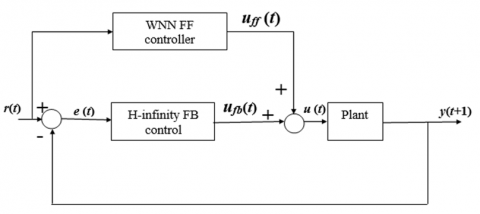
Both the FF and FB control techniques have distinct advantages and disadvantages. Particularly, the FB control approach is specifically distinguished by utilizing an H-infinity controller. Nevertheless, in the presence of a specific time delay in the controlled system, the FB controller will not immediately impact the system until a given duration of time has passed. The FB controller is a witness to the response time delay in the system, which can threaten performance control and stability [1]. On the contrary, the FF controller has an advantage as it can be used for anticipating the shifts of the reference signal and taking the required action on the concerned system immediately, resulting in faster convergence [9]. Within this work, the structure of control, namely the FB and FF, which is depicted in Figure 1, is accomplished this way: it involves the FF technology and the FB control technique. This feature gives the stem cell more holistic control and makes it more powerful and active.
Figure 1. Schematic representation of the FF-FB controller in the form of a block diagram
The robust intelligent control law for the proposed controller is:
$u=u_{f f}+u_{f b}$ (6)
where,
$u_{f f}=f^{-1}(g(x))$ (7)
where, $f^{-1}$ is a nonlinear function representing the inverse system dynamics. ANNs can be trained to acquire the nonlinear function of Eq. (7) and $u_{f b}$ is the FB H-infinity control action.
3.1 FF controller design
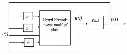
By training a neural network to function as an inverse model of the plant, direct inverse control (DIC) is achieved as a powerful method to control nonlinear systems. Figure 2 depicts the DIC's generalized design [13, 14].
Figure 2. Direct inverse control
Figure 2 represents the training process of the WNN as an FF controller, emphasizing the goal of achieving optimal control actions to track the desired reference signal accurately. It provides a conceptual overview of how the network learns to control the system through iterative optimization of its weights.
The training entails adjusting the WNN weights in order to reduce the integral squared error (ISE) criterion, as given below:
$J=0.5 * \sum_{t=1}^N(e(t))^2$ (8)
where,
$e(t)=r(t)-y(t)$ (9)
In Eq. (8), N denotes the number of time samples, whereas r(t) and y(t) in Eq. (9) correspond to the reference signal and the plant output, respectively. Nevertheless, a drawback of this control method is that the inverse modeling stage does not effectively minimize the output error, which refers to the discrepancy between the actual system output and the command signal. Therefore, the controller created using this approach may result in a consistent disparity between the desired and real outputs of the system [15]. Hence, to attain a desirable level of control precision, the FF controller is integrated with the FB controller, which will be further discussed in the subsequent section.
3.2 WNN structure
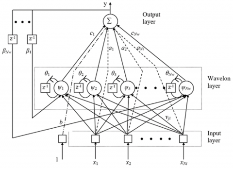
The structure of the proposed WNN for representing the FF controller is shown in Figure 3.
As depicted in Figure 3, the WNN consists of three layers, which are explained in the following [16, 17]:
The first layer, which is the input layer, is responsible for directly passing the input variables to the next layer without any modification. In this work, the input variables must have the following format to exploit the WNN as a FF controller.
$\begin{gathered}y(t+1), y(t), \ldots, y(t-n+1), \\ u(t-1), \ldots, u(t-m), r(t)\end{gathered}$ (10)
The mother wavelet, or the wavelet layer, is the second layer. Each node in this layer, referred to as a wavelon, receives three input variables, as shown in Figure 3, every input node possesses an associated weight, including a self-FB weight and a FB weight from the output node. These input variables are used by the $j^{t h}$ wavelon to determine the associated output, which is expressed as follows:
$\begin{gathered}z_j=d_j \\ \left(\sum_{i=1}^{N i} v_{j i} x_i+\psi_j(k-1) \cdot \theta_j+y(k-1) \cdot \beta_j\right)-t_j\end{gathered}$ (11)
where, the variables $d_j$ and $t_j$ represent the dilation and translation parameters, respectively. $N_i$ represents the node number in the input layer. $v_{j i}$ denotes the weight connecting the $i^{t h}$ input node and the $j^{\text {th }}$ wavelon. $x_i$ represents the i-th input variable. $\Psi(k-1)$ represents the network memory, which stores past information from the $j^{\text {th }}$ wavelon. $\theta_j$ represents the $j^{\text {th }}$ adjustable connection at the self-FB, which determines the rate of information storage. $y(k-1)$ denotes the output of the preceding network. $\beta_j$ denotes tghe weight parameter connecting output node to the $j^{\text {th }}$ wavelon.
Figure 3. Architecture of the WNN
The importance of selecting a suitable wavelet activation function is now well acknowledged, since it is considered equally crucial as picking the network design and the training approach [18]. In order to tackle this problem, a series of tests were carried out utilizing various wavelet functions. The RASP1 function exhibited superior approximation performance compared to other function types. Thus, the RASP1 function was utilized for calculating the output of the $j^{t h}$ wavelet using the following equation [19]:
$\Psi_j\left(z_j\right)=\frac{z_j}{\left(z_j^2+1\right)^2}$ (12)
The third layer consists of a single node that generates the ultimate output of the WNN structure utilizing the subsequent formula:
$y=\sum_{j=1}^{N w} c_j \psi_j\left(z_j\right)+\sum_{i=1}^{N i} a_i x_i+b$ (13)
where, $N_w$ is the number of wavelon layer nodes, $N_i$ represents the total number of nodes in the input layer, cj denotes the weight connection between the jth wavelon and output node, $a_i$ represents the weight that connects the ith input node to the output node, and finally, b represents a bias term for the output node. Based on the previously presented information, it is evident that the WNN structure has several adjustable weights, which may be encompassed under the set given below:
$S=\left[v_{j i} d_j t_j c_j \theta_j \beta_j a_i b\right]$ (14)
To utilize the WNN structure as the FF controller, it is necessary to train the weights mentioned in Eq. (14) by minimizing the ISE described in Eq. (8).
3.3 FB controller design
The next section delineates the design methodology of the FB controller for a system with a structure of [20, 21]:
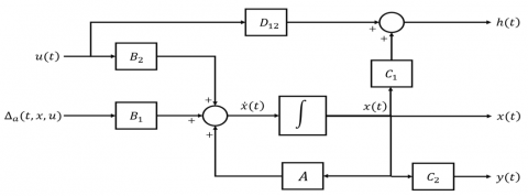
$\begin{gathered}\dot{x}(t)=A x(t)+B_1 \Delta_a(t, x, u)+B_2 u(t) ; x\left(t_o\right)=x_o \\ h(t)=C_1 x(t)+D_{12} u(t) \\ y(t)=C_2 x(t)\end{gathered}$ (15)
where,
$x(t) \in \Re^n$ is a vector of system states.
$\Delta_a(t, x, u) \in \Re^m$ is additive nonlinearity in this system.
$u(t) \in \Re^l$ is the input of control.
$e(t) \in \Re^q$ is vector of controlled outputs.
$y(t) \in \Re^p$ is the output vector of the system.
$A \in \Re^{n \times n}$ is the matrix of the system.
$B_1 \in \Re^{n \times m}$ represents the weight matrix of perturbation.
$B_2 \in \Re^{n \times l}$ is the matrix of control.
$C_1 \in \Re^{q \times n}$ is a system state weight matrix.
$D_{12} \in \Re^{q \times l}$ is a matrix with weights for regulating the inputs to the controller.
$C_2 \in \mathfrak{R}^{p \times n}$ is the weight matrix of the output.
The schematic representation of the dynamics of a nonlinear system in the controlled formulation, as described in Eq. (15), is depicted in Figure 4.
Figure 4. A block diagram illustrating the controllable form of a nonlinear system
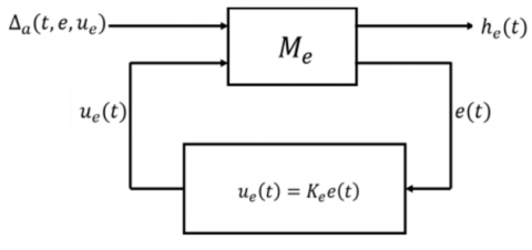
The typical arrangement of the all-encompassing state FB H-infinity control is illustrated in Figure 5.
Figure 5. The revised default setup of the control problem where $M_e$ represents the plant matrix [21]
To successfully execute a comprehensive state FB H-infinity control, it is necessary to have access to all the states of the system for FB, which indicates that:
$C_2=I . D_{11}, D_{21}$ and $D_{22}$ equals zero.
Thus, the plant matrix M is transformed into:
$M_e=\left[\begin{array}{ccc}A & B_1 & B_2 \\ C_1 & 0 & D_{12} \\ C_2 & 0 & 0\end{array}\right]$ (16)
The goal is to maintain the internal stability of the system so that ( $T_{h_e \Delta_a}$ ) stays within acceptable bounds, namely below a predefined threshold value of $\gamma$ [20]:
$\left\|T_{h_e \Delta_a}(j w)\right\|_{\infty} \leq \gamma$ (17)
where, $\gamma$ indicates that $\Delta_a\left(t, e, u_e\right)$ demonstrates linear development and has an upper bound, which the controller consistently handles [22].
The condition in Eq. (17) implies that [21]:
$\min _{u_e} \max _{\Delta_a} J\left(u_e, \Delta_a\right)<\infty$ (18)
and the function cost is [23]:
$J_{p s o}\left(\gamma, \rho, C_1\right)=\int_0^{\infty} e^2(t) d t$ (19)
The perturbation $\Delta_a$ aims to optimize the cost function $J\left(u_e, \Delta_a\right)$, whereas the control signal $u_e$ aims to reduce it.
The Lyapunov quadratic function is employed to derive the optimum controller and the worst-case perturbation gain matrices values, denoted as $K_e$ and $K_{\Delta}$, respectively [21].
The Lyapunov function and its derivative are defined as [24]:
$V(e)=e^T P_e e$ (20)
$\dot{V}(e)=-e^T Q_e e$ (21)
where, the matrices $P_e$ and $Q_e$, which are real symmetric matrices of size $\Re^{\omega \times \omega}$, define the definiteness of the functions $V(e)$ and $\dot{V}(e) . P_e$ must be positively definite, whereas $Q_e$ must be negatively definite.
The structure of the optimum control and the worst-case perturbation is as follows [25]:
$\Delta_a\left(t, e, u_e\right)=K_{\Delta} x(t) ; K_{\Delta} \in \Re^{m \times \omega}$ (22)
$u_e(t)=K_e(t)$ (23)
Evaluating Eq. (22) and Eq. (23) in Eq. (15), yields:
$\dot{x}=\left(A+B_1 K_{\Delta}+B_2 K_e\right) x$ (24)
Using assumption 3, the following equation will be obtained:
$h_e^T h_e=X^T\left(C_1^T C_1+K_e^T K_e\right) x$ (25)
Therefore,
$J\left(u_e, \Delta_a\right)=\int_0^{\infty}\left[e^T\left(C_{1_a}^T C_{1_a}+\rho K_e^T K_e-\gamma^2 K_{\Delta}^T K_{\Delta}\right) e\right] d t$ (26)
Now let:
$Q=\left(C_{1_a}^T C_{1_a}+\rho K_e^T K_e-\gamma^2 K_{\Delta}^T K_{\Delta}\right)$ (27)
The matrix Q must be positive definite. The optimum control law assumes that the system described in Eq. (27) is stable.
In order to get the most efficient cost function, Eq. (27) will be replaced with Eq. (18), resulting in:
$V(x)=-x^T\left(C_{1_a}^T C_{1_a}+\rho K_e^T K_e-\gamma^2 K_{\Delta}^T K_{\Delta}\right) x$ (28)
$x^T\left(C_{1_a}^T C_{1_a}+\rho K_e^T K_e-\gamma^2 K_{\Delta}^T K_{\Delta}\right) x=-\frac{d}{d t} x^T P x$ (29)
By performing the process of integration on both sides of Eq. (27) throughout the interval, we have:
$\begin{gathered}\int_0^{\infty} x^T\left(C_{1_a}^T C_{1_a}+\rho K_e^T K_e-\gamma^2 K_{\Delta}^T K_{\Delta}\right) x d t=-\int_0^{\infty} \frac{d}{d t} x^T P x d t\end{gathered}$ (30)
$J\left(u_e, \Delta_a\right)=-x(\infty)^T P x(\infty)-\left(-x(0)^T P x(0)\right)$ (31)
In order for the system described by Eq. (19) to remain stable under the control law, it is necessary that $x(\infty)=0$.
Hence, the most efficient cost function is:
$J^*=-x(0)^T P x(0)$ (32)
The matrix P, is positive definite, represents the evaluation of the Lyapunov equation given below:
$\left(A+B_1 K_{\Delta}+B_2 K_e\right) P^T+P\left(A+B_1 K_{\Delta}+B_2 K_e\right)=-Q$ (33)
$\begin{gathered}\left(A+B_1 K_{\Delta}+B_2 K_e\right) P^T+\left(A+B_1 K_{\Delta}+B_2 K_e\right)=-\left(C_{1_a}^T C_{1_a}+\rho K_e^T K_e-\gamma^2 K_{\Delta}^T K_{\Delta}\right)\end{gathered}$ (34)
$\begin{gathered}\left(A+B_1 K_{\Delta}+B_2 K_e\right) P^T+P\left(A+B_1 K 6_{\Delta}+B_2 K_e\right)\left(C_{1_a}^T C_{1_a}+\rho K_e^T K_e-\gamma^2 K_{\Delta}^T K_{\Delta}\right)=0\end{gathered}$ (35)
To determine the most efficient control law, it is necessary to derive Eq. (35) $K_e$ and make $\partial P / \partial K c i j=0$, and we get:
$K_e=-\frac{1}{\rho} B_{2_a}^T P_e$ (36)
As a result,
$u_e *=K_e x=-\frac{1}{\rho} B_{2_a}^T P_e x$ (37)
$\Delta_a\left(t, e, u_e\right)=K_{\Delta} x(t)=\frac{1}{\gamma^2} B_{1_a}^T P_e$ (38)
Now, Eq. (39) is solved, which is known as the H-infinity algebraic Riccati equation (HIARE) [26]:
$\begin{gathered}P_e A_a+A_a^T P_e+C_{1_a}^T C_{1_a}-P_e\left(\frac{1}{\rho} B_{2_a} B_{2_a}^T-\frac{1}{\gamma^2} B_{1_a} B_{1_a}^T\right) P_e=0_\omega\end{gathered}$ (39)
The purpose of training the WNN structure is to optimize the WNN parameters by reducing the discrepancy between the reference signal and the system's actual output. In particular, multiple changeable parameters in the FF controller need to be optimized. The parameters can be represented using the following settings:
$S=\left[v_{j i} d_j t_j c_j \theta_j \beta_j a_i b\right]$ (40)
For the WNN structure to achieve optimal performance, the parameters in Eq. (40) must be optimized using a suitable optimization approach. This work utilizes the particle swarm algorithm optimizer to determine these parameters.
The FB controller optimization is employed offline to tackle the optimization problem of the design procedure. The goal is to find the optimal value of $\rho$ and the optimal values of the elements in matrix $C_1$, such that the infinity norm of $\left\|T_{e \Delta_d}(j w)\right\|_{\infty}$ is less than or equal to the optimal value of $\gamma$. The selection of the optimization cost function is as follows:
$J_{p s o}\left(\gamma, \rho, C_1\right)=\int_0^{\infty} e^2(t) d t$ (41)
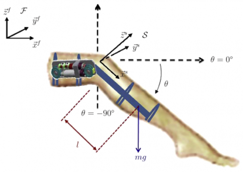
The control of a lower limb orthosis is applied at the knee joint level for rehabilitation purposes. Specifically, the control effort is applied to the system to guarantee the asymptotic stability and to make the system follow the desired trajectory in the rehabilitation process.
The efficacy of the suggested controller is demonstrated by considering the leg system's dynamic model, seen in Figure 6 and described by Eq. (39) [27]:
$J \ddot{\theta}=-T_g \cos (\theta)-A \operatorname{sign}(\dot{\theta})-B \dot{\theta}+u$ (42)
where,
$J$ is the inertial moment of the shank.
$\theta, \dot{\theta}$, and $\ddot{\theta}$ are the joint angular position, velocity, and acceleration, respectively.
The coefficients A and B represent the torques of solid and viscous friction, respectively.
Figure 6. The dynamic model of the leg system
The values of the parameters are illustrated in Table 1.
We can obtain the dynamic model by converting the dynamic model in terms of $x_1$ and $x_2$, where $x_1=\theta$ and $x_2=$ $\dot{\theta}: \dot{x}_1=x_2$.
Table 1. The system parameters
|
Parameter |
Value |
|
Inertia (J) |
0.4 Kg.m2 |
|
Solid friction coefficient (A) |
0.6 N.m |
|
Viscous friction coefficient (B) |
1 N.m.s.$\mathrm{rad}^{-1}$ |
|
Gravity torque ($\left.T_g\right)$) |
5 N.m |
$\begin{gathered}\dot{x}_2=-\frac{B}{J} x_2-\frac{T_g}{J} \cos \left(x_1\right)-\frac{A}{J} \operatorname{sign}\left(x_2\right)+\frac{1}{J} u \\ y=x_1\end{gathered}$ (43)
For the following nonlinear system:
$\begin{gathered}\dot{x}_1=x_2 \\ \dot{x}_2=-2.5 x_2-12.5 \cos \left(x_1\right)-1.5 \operatorname{sign}\left(x_2\right)+2.5 u \\ y=x_1\end{gathered}$ (44)
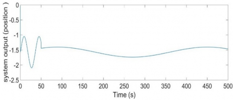
The system's open loop response, as described by Eq. (43), is depicted in Figure 7.
Figure 7. Open loop system output (degree)
Figure 8 shows the closed loop response of the system in Eq. (41).
Figure 8. Closed loop desired and actual leg system position before applying the controller
Figures 7 and 8 illustrate the response of the nonlinear system in both the open-loop and closed-loop configurations prior to the deployment of the recommended controller. The open-loop instability of the system and the critical closed-loop stability need the construction of a controller to stabilize the system and achieve the required performance. An additional part is required to enhance the control signal.
4.1 FB H-infinity controller design
For the system in Eq. (41), the H-infinity controller design is explained as:
Rearrange the state equation as:
$\begin{gathered}{\left[\begin{array}{l}\dot{x}_1 \\ \dot{x}_2\end{array}\right]=\left[\begin{array}{cc}0 & 1 \\ 0 & -2.5\end{array}\right]\left[\begin{array}{l}x_1 \\ x_2\end{array}\right]+\left[\begin{array}{l}0 \\ 1\end{array}\right] d(t)+\left[\begin{array}{c}0 \\ 2.5\end{array}\right] u} \\ y=x_1\end{gathered}$ (45)
where,
$d(t)=-5 \cos \left(x_1\right)-0.6 \operatorname{sign}\left(x_2\right)$ (46)
By using optimization, we need to get the optimal values of $\rho, \gamma$, and $C_1$. The optimal values are:
$\begin{gathered}\gamma_{\min }=0.8097 \\ \rho=0.1005 \\ C_1=\left[\begin{array}{ll}4.2105 & 7.1335 \\ 1.8473 & 3.2 .656\end{array}\right]\end{gathered}$ (47)
We must solve the Riccati equation as in Eq. (39).
The solution of this Riccati equation is:
$P=\left[\begin{array}{ll}10.7552 & 0.8089 \\ 0.8089 & 1.1609\end{array}\right]$ (48)
The state feedback control gain matrix is given as:
$K_e=[-47.9427-33.8615]$ (49)
Following that, the computed gain matrix is substituted in the control law defined in Eq. (37) that is applied to the primary system dynamics represented by Eq. (43).
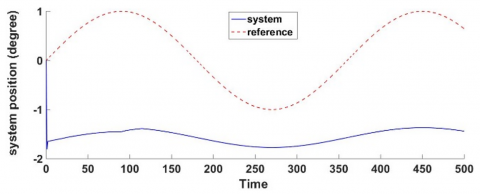
By choosing sin(t) as the reference signal, the state response is shown in Figure 9.
Figure 9. Desired and actual system position after applying the FB controller
Figure 10. Performance of the applied FB H-infinity controller
Figure 9 demonstrates the characteristics of the system's controlled closed-loop output trajectory, which precisely cannot track the trajectory of the command signal r(t)=sin(t). This means that an additional control part is required to achieve the desired specifications. Figure 10 illustrates the behavior of the control input, which is deemed unacceptable and ineffective in improving the performance and stability of the system. The existing data confirms that the suggested controller can achieve stability in the nonlinear system.
4.2 FF WNN controller
The WNN was trained to represent the FF controller to control the dynamics of the nonlinear system expressed in Eq. (43). The training signal is $\sin (t)$ as the reference signal.
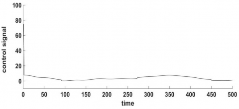
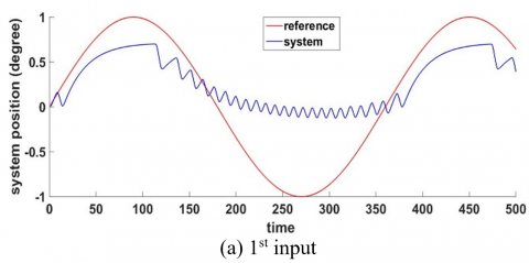
The suggested PSO method has been employed to optimize the parameters of the WNN structure . In order to optimize the process, a population consisting of 50 agents was used, and the maximum number of iterations was established at 500. In addition, the MRWNN structure consisted of six wavelons in its wavelon layer. Figure 11 demonstrates the effective control performance of the FF control technique in accurately following the reference signal. The experiment was conducted using 500 iterations and 50 particles.
Figure 11. System position of the controlled system with FF the controller
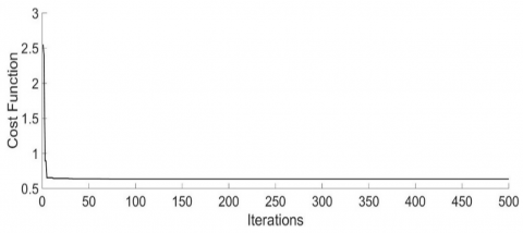
The WNN has effectively managed to regulate the dynamics of the nonlinear system, achieving an ISE value of 0.5707. Figure 12 depicts the successful reduction of the ISE by implementing the suggested PSO algorithm.
Figure 12. The best ISE against iterations
4.3 The combined FF-FB controller
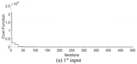
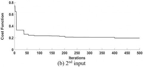
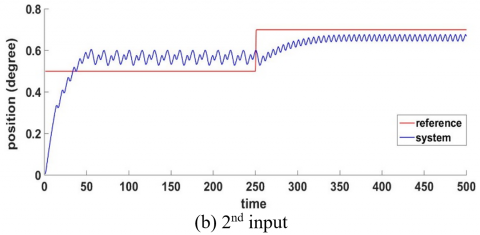
The effectiveness of the PSO algorithm in minimizing the cost function is demonstrated in Figure 13, where the integral square error is 0.0012 and 0.123 for two inputs respectively.
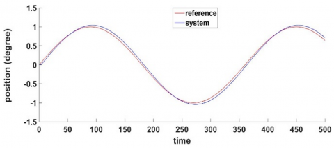
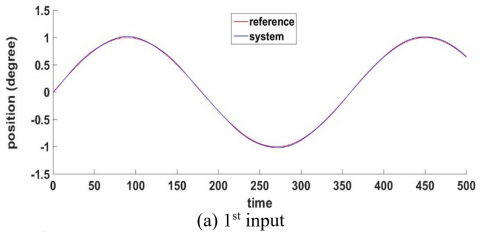
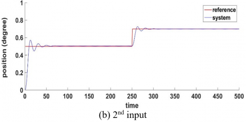
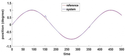
Figure 14 shows that the FF-FB control system achieved the desired control target by accurately tracking the required signal. The WNN, functioning as the FF controller with H-infinity as FB, has been effectively trained by accurately following the reference signal. The reference signal was a sine wave and muli step input.
FF-FB controller combined WNN and H-infinity controller structure as in Eq. (6).
For the FF optimization process, 50 agents were utilized to form each population, and the maximum number of iterations was chosen to be 500. In addition, six wavelons were used to constitute the wavelon layer in the WNN structure. Then PSO algorithm is then used to establish the controller’s optimality. Table 2 displays the optimization settings for the PSO algorithm. After the optimization process, the obtained optimal values and boundaries of the optimized parameters are illustrated in Table 3. The HIARE defined in Eq. (39) is then solved using the optimal values calculated, and its positive definite solution is computed as follows:
Figure 13. Attitude of the tracking error
Figure 14. Desired and actual leg system position after applying robust intelligent controller
Table 2. List of the pso algorithm settings
|
Optimization Setting |
Value |
|
Problem dimension (dim) (No. of parameters) |
59 (53 for FF and 6 for FB controller) |
|
Size of population |
50 |
|
No. of iterations |
500 |
|
No. of runs |
1 |
Table 3. The optimized parameters’ optimal values and bounds
|
Optimized Parameter |
Least Bound |
Upper Bound |
Optimum Value |
|
γ |
1 |
10 |
3.0221 |
|
ρ |
0.1 |
1 |
0.1123 |
|
c11 |
0 |
100 |
97.0483 |
|
c12 |
0 |
100 |
38.2477 |
|
c21 |
0 |
100 |
32.1956 |
|
c22 |
0 |
100 |
29.7672 |
$P=\left[\begin{array}{cc}333.4781 & 22.7490 \\ 2.7490 & 10.7639\end{array}\right]$ (50)
Then, the optimal gain matrix of the state FB controller has been determined using Eq. (36) as follows:
$K=[-186.6044-88.2937]$ (51)
The gains in Eq. (51) are then substituted in the control law Eq. (37) to be:
$u=186.6044 x_1+88.2937 x_2$ (52)
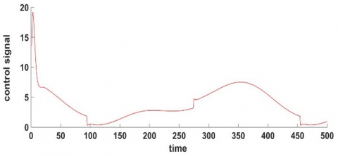
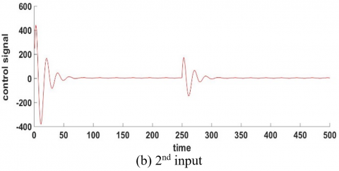
Afterwards, Eq. (52) is used and combined with $u_{f f}$ as in Eq. (6) to form the overall control signal, which is then applied to the system dynamics described in Eq. (43). Figure 14 illustrates that the proposed controller effectively endeavors to ensure that the system adheres to the desired trajectory. Two distinct inputs are used to evaluate the efficacy and robustness of the controller.
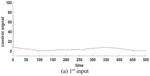
Figure 15 illustrates the impact of the control input on the system's performance and stability, showing that it is both permitted and effective.
Figure 15. Performance of the applied intelligent robust controller signal
In addition, Figure 13 demonstrates the quick disappearance of the tracking error norm, demonstrating that the controller has successfully fulfilled the asymptotic tracking requirement provided in Eq. (8).
Tests were made to investigate the robustness of the MRWNN-based FF-FB control structure to handle the effects of external disturbances. To perform this test on a nonlinear system with different inputs, a bounded disturbance with a magnitude of 30% of the system output was applied. The two periods are $150 \leq t \leq 155$ and $250 \leq t \leq 255$. Figure 16 reveals that the FF-FB control system has accommodated the effects of these unexpected disturbances on leg system position by recovering the desired response immediately after the influence of each disturbance. Figure 17 illustrates the effective control signal applied to the pendulum system to reject disturbances.
Figure 16. Disturbance rejection tests for leg system position
Figure 17. Performance of the applied control signal
Figure 18. Leg system position after applying (WNN-H-infinity) controller
The control performance of the WNN structure is compared with other neural network structures, such as the multilayer perceptron (MLP). This network was employed in FF, and the FB still in full state H-infinity control. The PSO was used to optimize the parameters of all the network and H-infinity controllers. For the MLP, six nodes were used in the hidden layer. Each of these nodes employs a sigmoidal activation function.
Following the same strategy in the FF-FB design for system tracking and decreasing the ISE. Figure 18 shows the system response controlled by this structure for two different control signal inputs controlled by the FF-FB control structure, where the FF controller was the MLP and the FB controller was the H-infinity controller.
The leg system under MLP control is shown in Figure 18 with its position trajectory, which is not tracking the necessary trajectory precisely. This suggests that the closed-loop system's stability and performance have not been reached by the controller, and this has approved the effectiveness of combined WNN and H-infinity controllers.
In this work, a FF-FB control structure was utilized to enhance the system's ability to handle nonlinear systems. The utilization of the WNN in the FF path represents an intelligent control strategy, where WNNs are known for their capability to model complex nonlinear systems. The nonlinear H-infinity controller in the FB loop suggests an emphasis on robustness and tracking. The PSO algorithm was utilized for optimizing the weights of the WNN and the parameters of the H-infinity controller. The efficacy of the FF-FB control system was demonstrated by simulation experiments conducted on a nonlinear leg movement model. Specifically, the system was evaluated based on control accuracy, the ability to track different reference signals, and its robustness against external disturbances. The overall conclusion is that the proposed FF-FB control system, incorporating the intelligent WNN in the FF path and the nonlinear H-infinity controller in the FB path, is effective in achieving the desired control performance for the nonlinear leg movement system. In particular, the control system was shown to be robust and accurate in tracking the reference signals. The comparative study has clearly highlighted the superiority of the FF (WNN)-FB(H-infinity) control structure over the MLP-Hinfinity controller. For future work, the proposed control approach will be implemented in real-time to adaptively control nonlinear control systems.
The authors express gratitude to the Ministry of Higher Education and Scientific Research, Iraq, and the University of Technology, Baghdad, for their financial assistance.
|
$v_i$ |
Velocity of the $i^{t h}$ particle |
|
$B_1$ and $B_2$ |
Weight matrices of the perturbation and control signals |
|
$C_1$ and $D_{12}$ |
Weight matrices for controlling the system states and control input |
|
$C_2$ |
System output weight matrix |
|
$J_{p s o}\left(\gamma, \rho, C_{1_a}\right)$ |
Cost function of the PSO algorithm |
|
$K_{\Delta}$ |
Gain matrix of the worst-case perturbation |
|
$K_e$ |
Gain matrix of the optimal robust controller |
|
$P_e$ and $Q_e$ |
Real symmetric positive definite matrices |
|
$A, B$, and $C$ |
System matrices |
|
$r(t)$ |
Desired command input |
|
$u(t)$ |
Control input |
[1] Sahoo, H.K., Dash, P.K., Rath, N.P. (2013). NARX model based nonlinear dynamic system identification using low complexity neural networks and robust H∞ filter. Applied Soft Computing, 13(7): 3324-3334. https://doi.org/10.1016/j.asoc.2013.02.007
[2] Omatu, S., Khalid, M., Yusof, R., Omatu, S., Khalid, M., Yusof, R. (1996). Neuro-control techniques. Neuro-Control and Its Applications, pp. 85-170. https://doi.org/10.1007/978-1-4471-3058-1_4
[3] Zhu, Z., Wang, R., Li, Y. (2017). Evaluation of the control strategy for aeration energy reduction in a nutrient removing wastewater treatment plant based on the coupling of ASM1 to an aeration model. Biochemical Engineering Journal, 124: 44-53. https://doi.org/10.1016/j.bej.2017.04.006
[4] Omatu, S., Khalid, M., Yusof, R., Omatu, S., Khalid, M., Yusof, R. (1996). Neuro-Control Applications. Springer London.
[5] Beijen, M.A., Heertjes, M.F., Butler, H., Steinbuch, M. (2016). Practical tuning guide to mixed feedback and feedforward control of soft-mounted vibration isolators. IFAC-Papersonline, 49(21): 163-169. https://doi.org/10.1016/j.ifacol.2016.10.536
[6] Sabahi, K., Teshnehlab, M. (2009). Recurrent fuzzy neural network by using feedback error learning approaches for LFC in interconnected power system. Energy Conversion and Management, 50(4): 938-946. https://doi.org/10.1016/j.enconman.2008.12.028
[7] Li, X., Zhu, H., Ma, J., Teo, T.J., Teo, C.S., Tomizuka, M., Lee, T.H. (2020). Data-driven multiobjective controller optimization for a magnetically levitated nanopositioning system. IEEE/ASME Transactions on Mechatronics, 25(4): 1961-1970. https://doi.org/10.1109/TMECH.2020.2999401
[8] Rigatos, G., Siano, P., Wira, P., Profumo, F. (2015). Nonlinear H-infinity feedback control for asynchronous motors of electric trains. Intelligent Industrial Systems, 1: 85-98. https://doi.org/10.1007/s40903-015-0020-y
[9] Yang, X., Yuan, J., Yuan, J., Mao, H. (2007). A modified particle swarm optimizer with dynamic adaptation. Applied Mathematics and Computation, 189(2): 1205-1213. https://doi.org/10.1016/j.amc.2006.12.045
[10] Ali, H.I., Noor, S.M., Bashi, S.M., Marhaban, M.H. (2010). Design of H-infinity based robust control algorithms using particle swarm optimization method. The Mediterranean Journal of Measurement and Control, 6(2): 70-81.
[11] Zirkohi, M.M., Fateh, M.M., Shoorehdeli, M.A. (2013). Type-2 fuzzy control for a flexible-joint robot using voltage control strategy. International Journal of Automation and Computing, 10: 242-255. https://doi.org/10.1007/s11633-013-0717-x
[12] Qaraawy, S., Ali, H., Mahmood, A. (2012). Particle swarm optimization based robust controller for congestion avoidance in computer networks. In 2012 International Conference on Future Communication Networks, Baghdad, Iraq, pp. 18-22. https://doi.org/10.1109/ICFCN.2012.6206865
[13] Amir, M.Y., Abbas, V. (2011). Modeling and neural control of quadrotor helicopter. Yanbu Journal of Engineering and Science, 2(1): 35-49. https://doi.org/10.53370/001c.23745
[14] Frye, M.T., Provence, R.S. (2014). Direct inverse control using an artificial neural network for the autonomous hover of a helicopter. In 2014 IEEE International Conference on Systems, Man, and Cybernetics (SMC), San Diego, CA, USA, pp. 4121-4122. https://doi.org/10.1109/SMC.2014.6974581
[15] Denaï, M.A., Palis, F., Zeghbib, A. (2007). Modeling and control of non-linear systems using soft computing techniques. Applied Soft Computing, 7(3): 728-738. https://doi.org/10.1016/j.asoc.2005.12.005
[16] Lutfy, O.F. (2018). Adaptive direct inverse control scheme utilizing a global best artificial bee colony to control nonlinear systems. Arabian Journal for Science and Engineering, 43(6): 2873-2888. https://doi.org/10.1007/s13369-017-2928-x
[17] Vo, C.P., To, X.D., Ahn, K.K. (2019). A novel adaptive gain integral terminal sliding mode control scheme of a pneumatic artificial muscle system with time-delay estimation. IEEE Access, 7: 141133-141143. https://doi.org/10.1109/ACCESS.2019.2944197
[18] Zainuddin, Z., Pauline, O. (2011). Modified wavelet neural network in function approximation and its application in prediction of time-series pollution data. Applied Soft Computing, 11(8): 4866-4874. https://doi.org/10.1016/j.asoc.2011.06.013
[19] Lutfy, O.F., Majeed, R.A. (2018). Internal model control using a self-recurrent wavelet neural network trained by an artificial immune technique for nonlinear systems. Engineering and Technology Journal, 36(7A): 784-791. https://doi.org/10.30684/etj.36.7A.11
[20] Ali, H.I., Shareef, Z. (2018). Full state feedback H2 and h-infinity controllers design for a two wheeled inverted pendulum system. Engineering and Technology Journal, 36(10A): 1110-1121. https://doi.org/10.30684/etj.36.10A.12
[21] Sinha, A. (2007). Linear Systems: Optimal and Robust Control. CRC Press.
[22] Rigatos, G., Siano, P., Abbaszadeh, M., Ademi, S., Melkikh, A. (2018). Nonlinear H-infinity control for underactuated systems: The Furuta pendulum example. International Journal of Dynamics and Control, 6: 835-847. https://doi.org/10.1007/s40435-017-0348-0
[23] Ali, H.I., Abdulridha, A.J. (2018). H-infinity based full state feedback controller design for human swing leg. Engineering and Technology Journal, 36(3A): 350-357. https://doi.org/10.30684/etj.36.3A.15
[24] Ogata, K., Yang, Y. (2002). Modern Control Engineering (Vol. 5). India: Prentice Hall.
[25] Xu, Z., Nian, X., Wang, H., Chen, Y. (2017). Robust guaranteed cost tracking control of quadrotor UAV with uncertainties. ISA Transactions, 69: 157-165. https://doi.org/10.1016/j.isatra.2017.03.023
[26] Stoorvogel, A.A. (1996). Stabilizing solutions of the H∞ algebraic Riccati equation. Linear Algebra and Its Applications, 240: 153-172. https://doi.org/10.1016/0024-3795(94)00195-2
[27] Rifai, H., Hassani, W., Mohammed, S., Amirat, Y. (2011). Bounded control of an actuated lower limb orthosis. In 2011 50th IEEE Conference on Decision and Control and European Control Conference, Orlando, FL, USA, pp. 873-878. https://doi.org/10.1109/CDC.2011.6160993