Hayder Al-Shuka*![]() | Ahmed H. Kaleel
| Ahmed H. Kaleel![]()
© 2024 The authors. This article is published by IIETA and is licensed under the CC BY 4.0 license (http://creativecommons.org/licenses/by/4.0/).
OPEN ACCESS
Bipedal locomotion requires a multi-level control strategy for balance and tracking, with the zero-moment point (ZMP) serving as a heuristic balance criterion. Maintaining the ZMP location within the stability margin indicates stability, but ankle joint actuation behavior restrictions are required. This paper focuses on whole-body control of a bipedal robot, considering control input limitations. Two dynamical models of bipedal dynamics are introduced, integrating center-of-mass (CoM)-based dynamics with joint space dynamics. The controlled outputs are the CoM position and joint displacements, while the control inputs are the ZMP position and joint torques. Anti-input saturation control is considered to ensure safe values for the control inputs, especially for the ZMP and ankle joint torque signals. A decentralized adaptive approximation control (DAAC) with a saturation compensator is designed. The stability of the proposed controller is proven using Lyapunov theory. Simulation experiments are conducted on a planar 6-degrees-of-freedom (DOF) bipedal robot. The results demonstrate the robustness of the control architecture even under a disturbance torque of 10 N.m., ensuring safe stability margins for the ZMP and precise tracking for the multi-DOF bipedal system.
bipedal locomotion, whole-body control, zero-moment point, decentralized adaptive control, bipedal dynamics
Dynamic mobility of legged robots across difficult terrains requires considering the robot's dynamics, actuation restrictions, and interaction with the environment. Legged robots now focus on movement and balancing, with the zero-moment point (ZMP) or center of pressure (CoP) being crucial for balancing [1-4]. The humanoid research community is increasingly interested in the complex motion control tasks of multi-DOF humanoid robots, particularly those with hyper-DOF systems. New developments in locomotion control, tested on quadrupeds and bipeds, often rely on lower-dimensional models or quasi-static assumptions, restricting the robot's dynamic movement [5, 6]. Optimization-based techniques, like non-linear model predictive control (MPC), can be used to plan and control movement while accounting for the robot's entire dynamics. However, if not warm-started, the solver may become trapped in local minima [7, 8].
The center of mass (CoM) of a multi-DOF system is a promising controllable variable in Cartesian space for mobile robots, including biped humanoid robots, requiring a direct target location. To address this, a strategy based on whole-body control (WBC) is used for dynamic movements. Full-body motion control is based on assigning proper degrees of freedom for motion tasks, originating from managing redundant manipulators. It addresses tracking performance, joint limitations, singular configurations, and self-collision avoidance [9]. WBC allows for decoupling control and motion planning, executing multiple tasks while maintaining the robot's behavior. It uses the robot's entire range of motion and degrees of freedom to distribute motion duties across joints, optimizing tasks while considering actuation, interaction, and system dynamics. WBC uses real-time optimization by describing robot dynamics as linear constraints with a convex cost function [10-14]. Hirai et al. [15] suggested and successfully implemented ZMP modulation control of CoM on their real humanoid robots. Position-controllable humanoids are proposed in the studies [16, 17], where the concept is extended to whole-body motion control. Hyon et al. [18] suggested the use of torque-controllable robots and a resolved acceleration controller for direct acceleration control of CoM in multi-DOF humanoid robots. By using the weighted pseudoinverse of the Jacobian from ZMP to CoM, the redundancy problem was resolved. A novel task space controller for force-controllable humanoids is proposed in the study [19]. Caron et al. [20] developed a whole-body admittance controller that integrates end-effector and CoM methods, along with quadratic programming wrench distribution, to improve walking stabilization in linear inverted pendulum tracking [21]. Ramuzat et al. [22] compared three control techniques on the TALOS Humanoid Robot, focusing on solving locomotion problems such as ascending stairs, walking on flat and uneven ground, and walking on both. The first used a hierarchical quadratic program at the velocity level, the second used a weighted quadratic program called Task Space Inverse Dynamic (TSID) at the acceleration stage, and the last used torque level instead.
In light of the above, the limits of the control inputs are often integrated with the WBC using quadratic programming optimization; however, a few studies have considered bounded control (or anti-input saturation) with low-level control for a bipedal robot that has fewer computations and is preferred for real-time applications. Robot control input bounds play a crucial role in maintaining stability and safety during a robot's operation by setting essential limits on the values provided to the actuators. These bounds, which consider factors such as torque, speed, and environmental restrictions, are crucial for regulating the motion of the robot. The maximum and minimum values assigned to each actuator are determined based on physical constraints and performance requirements. Recently, Ghoreishi et al. [23] have proposed an anti-windup double hyperbolic sliding mode controller for a three-legged robot under torque constraints. Researchers are working on developing controllers for actuators with practical limits like saturation, dead zone, and hysteresis to improve closed-loop system performance and safety. Two approaches include changing the control effort signal and building an auxiliary system to specify tracking errors, aiming to solve these constraints and enhance closed-loop system performance [24-26]. The contributions of our paper are outlined as follows:
The study focuses on modeling a bipedal robot using the WBC, integrating centroidal dynamics with joint space dynamics. Control inputs include ground reaction forces (GRFs) and joint torques, while output variables are joint states and CoM states. Bounded control is required due to constraints on the ankle joints and the GRF values. An anti-input saturation control is combined with the proposed control law. A unified control law is designed for joint tracking and compensation of the ZMP error. The control architecture is based on the adaptive function approximation technique, considering uncertainty in bipedal parameters and dynamics. The key idea is that every uncertain term can be represented using orthogonal basis functions such as Chebyshev polynomials, Fourier series, neural network approximators, etc.; see the studies [27-30] for more details. The adaptive law for the weighting coefficients is designed using Lyapunov theory to ensure stability based on the passivity condition. Simulation experiments are implemented on a 6-link bipedal robot in the single-support phase of SSP, considering adaptive and non-adaptive case studies. The results show the effectiveness of the proposed controller.
The rest of the paper is structured as follows: Section 2 introduces WBC dynamic modeling. The bipedal robot's control over locomotion is thoroughly explained in Section 3. Results are presented in Section 4, and conclusions and recommendations for further work are made in Section 5.
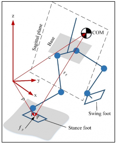
This section integrates Cartesian centroid models with joint space dynamics to control bipedal locomotion. Two robot models have been developed: Model 1, utilizing CoM (trunk) dynamics and GRF as control inputs, and Model 2, which reformulates centroid dynamics with ZMP locations as input signals; refer to Figure 1. The point p is the location of the ZMP where the contact force $f_p$ is applied. The base frame is assumed to be placed at the CoM (trunk). The base frame can be positioned at the fixed-stance foot with more simplified dynamics. In Model 1, the floating base frame is positioned at the trunk (CoM), while in Model 2, there is a fixed base frame at the stance ankle. The (n+6)-DOF dynamics of a bipedal model are decoupled for control tasks aimed at complete control of bipedal locomotion. The following assumptions are imposed [31, 32].
Assumption 1: Due to the brief double support phase, the gait cycle comprises only a single support phase, SSP.
Assumption 2: The ZMP location is maintained within the stance sole by fixing the stance foot. This assumption is crucial to preventing deviations in the ZMP beyond the stability margin.
Assumption 3: There is no variation in the height of the trunk (CoM) during locomotion.
Assumption 4: The bipedal robot is governed by floating-based dynamics, with the CoM as a floating base with neglected rotational dynamics.
Figure 1. A bipedal model in the single contact locomotion
Remark 1. The main focus of the control problem is to track the desired joint trajectories of a bipedal robot while also keeping within bounds on ZMP values when tracking the desired CoM references. Thus, opting to designate the CoM as a floating base is the optimal approach. By designating the CoM as a floating base and disregarding rotational dynamics, the humanoid system becomes uncoupled, separating the CoM dynamics from the joint space dynamics. Selecting a different component as a floating base can complicate control and motion planning processes. Therefore, if a bipedal system is constructed as a coupled system, it will necessitate additional efforts in motion planning, stabilization, and low-level control. Such tasks are not within the scope of this study.
2.1 Model 1
This model is widely used in the literature and includes CoM dynamics combined with link dynamics in joint space with base frame positioned at the trunk or the CoM; see, e.g., [31]. The equation of motion describing the exact full-body dynamics with a single contact point is expressed as [9, 31, 32].
$\left[\begin{array}{lll}M_{11} & M_{12} & M_{13} \\ M_{21} & M_{22} & M_{23} \\ M_{31} & M_{32} & M_{33}\end{array}\right]\left[\begin{array}{c}\ddot{r}_c \\ \ddot{\omega}_c \\ \ddot{\theta}\end{array}\right]+\left[\begin{array}{c}\eta_1 \\ \eta_2 \\ \eta_3\end{array}\right]=\left[\begin{array}{c}0_3 \\ 0_3 \\ \tau\end{array}\right]+\left[\begin{array}{c}I_3 \\ {\left[r_p^c \times\right]} \\ J^T\end{array}\right] f_p$ (1)
where, $M_{i j}$ is an inertia matrix, $r_c=\left[c_x, c_y, c_z\right]^T$ is the position vector of the floating base, $\omega_c=\left[\omega_x, \omega_y, \omega_z\right]^T$ is the angular velocity of the floating base, $\eta_i$ is an nonlinear vector including the Coriolis, centripetal and gravity effect, $I_3$ is an $3 \times 3$ identity matrix, $0_3$ is a $3 \times 1$ null vector, $\theta \in R^n$ is the angular displacement vector of the target biped, $\tau \in R^{n_a}$ is the control joint torques, $n_a$ is the number of actuated joints, $J \in$ $R^{3 \times n}$ is the Jacobian matrix from the floating base to the contact point $P$.
The following points should be noted:
$\underbrace{\left[\begin{array}{cc}M & 0_{2 \times n} \\ 0_{n \times 2} & H\end{array}\right]}_D \underbrace{\left[\begin{array}{c}\ddot{r}_c \\ \ddot{\theta}\end{array}\right]}_{\ddot{q}}+\left[\begin{array}{l}\eta_1 \\ \eta_2\end{array}\right]=\left[\begin{array}{c}0_{2 \times 1} \\ \tau\end{array}\right]+\left[\begin{array}{c}I_{2 \times 2} \\ 0_{n \times 2}\end{array}\right] f_p=\underbrace{\left[\begin{array}{c}f_p \\ \tau\end{array}\right]}_u$ (2a)
with
$\underbrace{\left[\begin{array}{c}\eta_1 \\ \eta_2\end{array}\right]=\left[\begin{array}{cc}0_{2 \times 2} & 0_{2 \times n} \\ 0_{n \times 2} & C_\theta\end{array}\right]}_C \underbrace{\left[\begin{array}{l}\dot{r}_c \\ \dot{\theta}\end{array}\right]}_{\dot{q}}+\underbrace{\left[\begin{array}{l}g_c \\ g_\theta\end{array}\right]}_g$ (2b)
The following benefits arise from the decoupling of the CoM dynamics from the joint space robot dynamics in Eq. (2):
2.2 Model 2
This model focuses on the bipedal robot as a rooted system at the neglected dynamics stance foot, similar to setting the floating base frame at the grounded stance foot. It includes ZMP-CoM dynamics and the robot's joint space dynamics, expressing the following mathematical relationship between ZMP position and CoM [33, 34].
$x_{Z M P}=\left(-\frac{c_z}{\ddot{c}_z+g}\right) \ddot{c}_x+c_x-\frac{\tau_{c y}}{m_c\left(\ddot{c}_z+g\right)}$ (3a)
$y_{Z M P}=\left(-\frac{c_z}{\ddot{c}_z+g}\right) \ddot{c}_y+c_y+\frac{\tau_{c x}}{m_c\left(\ddot{c}_z+g\right)}$ (3b)
where, $g=9.81 \mathrm{~m} / \mathrm{s}^2, p=\left[\begin{array}{lll}x_{Z M P} & y_{Z M P} & z_{Z M P}\end{array}\right]^T$ is the ZMP position vector with $z_{Z M P}$ setting to zero assuming flat ground, and $\left[\begin{array}{lll}\tau_{c x} & \tau_{c y} & \tau_{c z}\end{array}\right]^T$ is the rate of angular momentum about the CoM. Eq. (3) is important in stabilization control of bipedal locomotion and it is similar to the first two equations in Eq. (2) related to the CoM dynamics. Eq. (3) can be reformulated in a matrix form as
$\bar{M} \ddot{c}+g_\alpha=u_c$ (4)
where,
$\begin{gathered}\bar{M}=\left[\begin{array}{cc}\left(-\frac{c_z}{\ddot{c}_z+g}\right) & 0 \\ 0 & \left(-\frac{c_z}{\tilde{c}_z+g}\right)\end{array}\right], g_\alpha=\left[\begin{array}{c}c_x-\frac{\tau_{c y}}{m_c\left(\ddot{c}_z+g\right)} \\ c_y+\frac{\left.\tau_{c x}\right)}{m_c\left(\ddot{c}_z+g\right)}\end{array}\right], u_c=\left[\begin{array}{l}x_{Z M P} \\ y_{Z M P}\end{array}\right]\end{gathered}$
Incorporating Eq. (4) with the bipedal model in joint space dynamics, considering single point contact, i.e., the SSP, yields
$\underbrace{\left[\begin{array}{cc}\bar{M} & 0_{2 \times n} \\ 0_{n \times 2} & \bar{H}\end{array}\right]}_D \underbrace{\left[\begin{array}{c}\ddot{c} \\ \ddot{\theta}\end{array}\right]}_{{\ddot{q}}}+\underbrace{\left[\begin{array}{cc}0_{2 \times 2} & 0_{2 \times n} \\ 0_{n \times 2} & \bar{C}_\theta\end{array}\right]}_C \underbrace{\left[\begin{array}{c}\dot{c} \\ \dot{\theta}\end{array}\right]}_{\dot{q}}+\underbrace{\left[\begin{array}{l}g_\alpha \\ \bar{g}_\theta\end{array}\right]}_g=\left[\begin{array}{c}0_2 \\ \tau\end{array}\right]+\left[\begin{array}{c}I_{2 \times 2} \\ 0_{n \times 2}\end{array}\right] u_c=\underbrace{\left[\begin{array}{c}u_c \\ \tau\end{array}\right]}_u$ (5)
The following points should be noted, despite the similarities between Eqs. (2) and (5):
The WBC aims to maintain the balance of a bipedal robot during environmental interaction. It divides motion tasks into trunk (CoM) tasks and lower-limb tasks. The trunk task uses Cartesian-based dynamics and control to stabilize trunk orientation and CoM location. The lower-limb task controls the trajectory of the swing foot using joint space dynamics to position the foot with sufficient clearance from the ground. In the following, a decentralized adaptive control based on passivity is described in detail to stabilize and track the bipedal motion. Recalling Eqs. (2) and (5), which can be expressed in a unified form as
$D \ddot{q}+C \dot{q}+g=u$ (6)
with nomenclature defined in (2) and (5). The system in (6) has the following properties and assumptions.
Property 1. Uniform bounds apply to the gravity vector, the Coriolis, centrifugal, and inertia matrices.
These bounds on physical parameters can be determined using a CAD/CAM model for the bipedal robot or using one of the system identification approaches; see the study [33] for more details.
Property 2. If $C(q, \dot{q})$ is specified using the Christoffel symbols then the matrix $N=\dot{D}-2 C$ is a skew-symmetric matrix.
Control input signals in Eq. (2) are subjected to the following constraints:
$u_i=\operatorname{sat}\left(\beta_i\right)=\left\{\begin{array}{c}u_{i_{\max }}, \beta_i \geq u_{i_{\max }} \\ \beta_i, u_{i_{\min }}<\beta_i<u_{i_{\max }} \\ u_{i_{\min }}, \beta_i \leq u_{i_{\min }}\end{array}, i=1,2,3, \ldots, m\right.$ (7)
The control tolerance vector's components, $\alpha_i$, can be expressed as
$\alpha_i=\left\{\begin{array}{c}u_{i_{\max }}-\beta_i, \beta_i \geq u_{i_{\max }} \\ 0, u_{i_{\min }}<\beta_i<u_{i_{\max }} \\ u_{i_{\min }}-\beta_i, \beta_i \leq u_{i_{\min }}\end{array}\right.$ (8)
A decoupled formulation of Eq. (6) is as follows:
$d_{i i}(q) \ddot{q}_i+c_{i i}(q, \dot{q}) \dot{q}_i+\kappa_i(q, \dot{q})=u_i$ (9a)
with
$\kappa_i(q, \dot{q})=\sum_{\substack{j=1 \\ j \neq i}}^m d_{i j}(q) \ddot{q}_j+\sum_{\substack{j=1 \\ j \neq i}}^m c_{i j}(q, \dot{q}) \dot{q}_j+g_i(q)$ (9b)
For uncertain dynamics, the following control law is chosen:
$\begin{aligned} & \hat{d}_{i i}(q) \ddot{q}_{r_i}+\hat{c}_{i i}(q, \dot{q}) \dot{q}_{r_i}+\mu_i S_i+\hat{\kappa}_i(q, \dot{q}) +\gamma_i \operatorname{sgn}\left(s_i\right)=u_{i_i}=\hat{\alpha}_i+\beta_i\end{aligned}$ (10a)
where,
$\dot{q}_{r_i}=\dot{q}_{d_i}+\lambda_i\left(q_{d_i}-q_i\right)$ (10b)
where, $\mu_i$ is a positive feedback gain, $\lambda_i$ is a time constant parameter, $\gamma_i$ is a sliding term gain and the subscripts $\mathrm{r}$ and $\mathrm{d}$ stands for the required and desired references. To estimate the uncertainty in Eq. (10), adaptive control based on FAT is utilized. The uncertainty is estimated using an orthogonal polynomial approximator, presuming that the uncertain dynamic matrices and vectors are functions of time. Thus, the control law in Eq. (11) becomes
$\begin{aligned} & \underbrace{\hat{w}_{d_i}^T \psi_{d_i}}_{d_i} \ddot{q}_{r_i}+\underbrace{\hat{w}_{c_i}^T \psi_{c_i}}_{c_i} \dot{q}_{r_i}+\eta_i s_i+\underbrace{\hat{w}_{\kappa_i}^T \psi_{\kappa_i}}_{\kappa_i}-\underbrace{\hat{w}_{\alpha_i}^T \psi_{\alpha_i}}_{\alpha_i} +\gamma_i \operatorname{sgn}\left(s_i\right)=\beta_{d_i}\end{aligned}$ (11)
where, $w_{(.)} \in R^{n_o}$ and $\psi_{(.)} \in R^{n_o}$ represents the weighting coefficients and orthogonal basis function vectors, respectively, with $n_o$ denoting the number of basis function terms. The following closed-loop dynamics result from deducting Eq. (11) from Eq. (9):
$\begin{aligned} & d_i \dot{s}_i+c_i s_i+\mu_i s_i+\gamma_i \operatorname{sgn}\left(s_i\right)= -\widetilde{w}_{d_i}^T \psi_{d_i} \ddot{q}_{r_i}-\widetilde{w}_{c_i}^T \psi_{c_i} \dot{q}_r-\widetilde{w}_{\kappa_i}^T \psi_{\kappa_i}+\widetilde{w}_{\alpha_i}^T \psi_{\alpha_i} +\left(\beta_i-\beta_{d_i}\right)+\varepsilon_i\end{aligned}$ (12)
where, $\varepsilon_i$ is error in the approximation. Achieving stable closed-loop dynamics requires the selection of the following updated adaptive laws.
$\begin{aligned} & \dot{\hat{w}}_{d_i}=\Omega_{d_i} \psi_{d_i} \ddot{q}_{r_i} s_i \\ & \dot{\hat{w}}_{c_i}=\Omega_{c_i} \psi_{c_i} \dot{q}_{r_i} s_i \\ & \dot{\hat{w}}_{\kappa_i}=\Omega_{\kappa_i} \psi_{\kappa_i} s_i \\ & \dot{\hat{w}}_{\alpha_i}=-\Omega_{\alpha_i} \psi_{\alpha_i} s_i\end{aligned}$ (13)
where, $\Omega_{(.)} \in R^{n_o \times n_o}$ is the adaptation's positive-definite gain matrix. The stability of the suggested control structure is demonstrated by the following theorem.
Theorem 1. Given $\beta_{d_i}=\beta_i$, the dynamics of the bipedal subsystems in (9), the control laws in Eq. (10), the corresponding closed-loop dynamics in Eq. (12), and the associated update adaptive laws in Eq. (13) are all stable in light of Barbalat's lemma [27].
Proof.
Consider the following non-negative function, $V_i$, for the ith subsystem:
$\begin{aligned} & V_i=\frac{1}{2} d_i s_i^2+\frac{1}{2} \widetilde{w}_{d_i}^T \Omega_{d_i}^{-1} \widetilde{w}_{d_i}+\frac{1}{2} \widetilde{w}_{c_i}^T \Omega_{c_i}^{-1} \widetilde{w}_{c_i} +\frac{1}{2} \widetilde{w}_{\kappa_i}^T \Omega_{\kappa_i}^{-1} \widetilde{w}_{\kappa_i}+\frac{1}{2} \widetilde{w}_{\alpha_i}^T \Omega_{\alpha_i}^{-1} \widetilde{w}_{\alpha_i}\end{aligned}$ (14)
Calculating the time derivative of Eq. (14) and inserting Eq. (12) into it yields
$\begin{aligned} & \dot{V}_i=\frac{1}{2}\left(\dot{d}_i-2 c_i\right) s_i^2-\mu_i s_i^2-\gamma_i s_i \operatorname{sgn}\left(s_i\right)+ \varepsilon_i s_i-\tilde{w}_{d_i}^T\left(\Omega_{d_i}^{-1} \dot{\hat{w}}_{m_i}+\psi_{d_i} \ddot{q}_{r_i} s_i\right) -\tilde{w}_{c_i}^T\left(\psi_{c_i} \dot{q}_{v_i} s_i+\Omega_{c_i}^{-1} \dot{\hat{w}}_{c_i}\right)-\tilde{w}_{\kappa_i}^T\left(\varphi_{\kappa_i} s_i+\Omega_{\kappa_i}^{-1} \dot{\hat{w}}_{\kappa_i}\right)\end{aligned}$ (15)
Combining the adaptive laws in Eq. (13) with the passivity property results in
$\dot{V}_i=-\mu_i s_i^2-\gamma_i s_i \operatorname{sgn}\left(s_i\right)+\varepsilon_i s_i$ (16)
Assume that $\gamma_i \geq\left|\varepsilon_i\right|+\sigma_i$, it leads to
$\dot{V}_i \leq-\mu_i s_i^2-\sigma_i s_i<0$ (17)
Eq. (17) is asymptotically stable according to Barbalat’s lemma.
Remark 2. The control input vector in Eq. (6) consists of ZMP coordinates and joint torques. To maintain stable and balanced locomotion, the ZMP location within the stance foot is crucial; otherwise, the bipedal system may become unstable. Hence, the ZMP bounds are set based on the foot dimension with a safety margin. Ankle joint torque significantly influences the robot's balance during locomotion as it directly correlates with the ZMP location; hence, the torque must be restricted to guarantee safe motion. Refer to pages 98 of the study [32] and the study [35] for further information.
The section conducts some simulation experiments to validate the proposed control architecture on a planar 6-link bipedal robot shown in Figure 2, using physical parameters from Table 1.
The simulation experiments utilized the MATLAB/SIMULINK 2023b package with a fixed time step size of 0.01s employing the Dormand-Prince (RK8) formula offering eighth-order accuracy. There are two options for ground-foot contact. One approach involves establishing a compliant contact between the stance foot and ground using a mass-spring-damper model, necessitating an assessment of ground stiffness and damping as outlined in the studies [36-38]. Alternatively, a simplified model assumes the bipedal robot is affixed to the massless stance foot, disregarding ankle height. In this scenario, the ground interacts with the bipedal robot through the actuated ankle joint, a technique adopted in our simulations. One-level control is intended to stabilize bipedal locomotion, which is an intriguing point. The desired gait patterns are 0° for the swing foot and 90° for the legs, thighs, and trunk links. When examining the sagittal plane alone, this position satisfies the equilibrium for bipedal motion. For simulation, two scenarios are chosen: Scenario 1 addresses tracking control and stabilization, taking input saturation into account, and Scenario 2 makes the assumption of an arbitrary disturbance force in the presence of an input saturation compensator. An impulse torque of 10 N.m. is applied to the bipedal model to perturb the dynamic response of the bipedal system.
Table 1. Physical specifications of the bipedal robot
|
Components |
Moments of Inertia [kgm2] |
Lengths [m] |
Masses [kg] |
|
Foot |
0.016 |
0.3 |
2 |
|
Shank |
0.06 |
0.45 |
3.6 |
|
Thigh |
0.06 |
0.45 |
3.7 |
|
Trunk |
0.145 |
0.45 |
10 |
The following assumptions are imposed in the simulation:
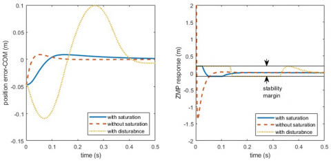
Figure 2. The CoM position error and the ZMP control inputs considering three simulation scenarios
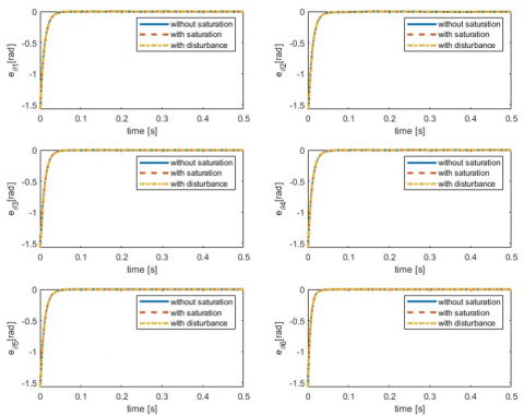
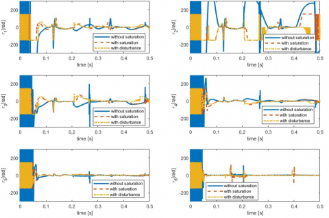
Figures 3 and 4 show the CoM position error and the ZMP position signals, respectively. The ZMP position is considered here as a control input with boundary limits based on the size of the stance foot. The period of the swing phase is taken as 0.5 seconds. It should be noted that the position error for the CoM will be larger in the presence of a disturbance torque with a larger value for control inputs. However, the availability of saturation compensators solves the problem of ensuring the ZMP limits within the stable region. The disturbance force causes an unrealistic shift in the ZMP location, indicating that the system is beyond the stability margin and unstable. However, the position error of the CoM approaches zero after 0.4 s; see Figure 3. Nonetheless, bounded control is crucial for stabilizing the system. The position error with the saturated control inputs for the biped joints is depicted in Figures 3 and 4 respectively. The position error asymptotically approaches zero in the steady-state region. In fact, the tracking position error is increased by the use of the anti-input saturation compensator. Nonetheless, its presence is crucial in achieving stable locomotion, as the constrained ankle torque values are relevant to ZMP stability. The CAD-CAM model proves to be beneficial in offering a comprehensive insight into the system's dynamic response and certain physical parameters of the target system. In our simulation tests, the joint torque limitations are arbitrarily chosen to assess the efficiency of our proposed controller, ranging from -150 to 150 N.m. Several key factors influence the control input limits, including foot size, ground incline, and the CoM location of the target bicycle, determined by system configurations and modeling. These factors impact the ZMP limit, ankle torque values, as well as the robot's speed.
Figure 3. Position error for biped joints considering three scenarios
Figure 4. Control inputs considering three scenarios. The limits on the joint actuators are set to 150 N.m. to -150 N.m.
The following important points should be noted:
This paper discusses the development of a decentralized adaptive approximation control that addresses saturation problems in control inputs. The key idea is to design a unified control based on whole-body dynamics, integrating ZMP-CoM dynamics with the bipedal multibody system. Further work is needed to address the multi-phase gait cycle and solve discontinuous dynamic responses. The integration of a saturation compensator with the control law enhances balance and safe locomotion. The human locomotion system is seen as a valuable model for biped robots due to its similarities. Recent advancements in biped robotics are centered on achieving robotic walking that closely mimics human gait. Human gait consists of two main phases: stance (DSP) and swing (SSP). Foot rotation is a key characteristic of human walking, involving heel-strike and toe-off movements as primary phases. This ability enables biped robots to reproduce human gait patterns, enhancing their walking efficiency and safety. Toe-off and heel-strike actions can modify the system's degree of freedom (DOF), leading to either under- or over-actuation. Consequently, a complete gait cycle is characterized by three phases: full actuation, under-actuation, and over-actuation when comparing DOF values with actuated joints. The challenge with multi-phase locomotion is the discontinuous dynamic response during walking phases due to variations in configurations and dynamical behaviors for each phase. Implementing whole-body dynamics with a floating-base dynamic model represented by the trunk proves to be a robust approach for multi-contact modeling. Thus, upcoming research will concentrate on whole-body motion planning and control while considering the entire gait cycle. It is essential to conduct a comparative analysis between floating-base dynamics and conventional methods that employ a discrete model for each walking sub-phase.
|
$\left(c_x, c_y, c_z\right)$ |
the coordinates of the floating base |
|
CoM |
center of mass |
|
CoP |
center of pressure |
|
DAAC |
a decentralized adaptive approximation control |
|
DOF |
degrees of freedom |
|
DSP |
double support phase |
|
FAT |
function approximation technique |
|
GRF |
ground reaction force |
|
MPC |
model predictive control |
|
SSP |
single support phase |
|
WBC |
whole body control |
|
$c_\theta$ |
a Coriolis and centripetal matrix related to the joint space dynamics |
|
$f_p$ |
a ground reaction force $\in R^3$ applied to point p |
|
H |
an inertia sub-matrix associated with joint space dynamics |
|
$I_{n \times n}$ |
an identity matrix |
|
M |
an inertia matrix associated with com dynamics |
|
$M_{i j}$ |
an inertia sub-matrix |
|
n |
number of degrees of freedom |
|
$n_o$ |
number of terms of an orthogonal basis function |
|
$n_a$ |
number of actuated joints |
|
$O_{n \times n}$ |
a null matrix |
|
p |
position vector of the ZMP coordinates |
|
$V_i$ |
Lyapunov function |
|
$r_c$ |
a positive vector $\in R^3$ of a floating base |
|
$s_i$ |
a sliding velocity variable |
|
$u_i$ |
control input for subsystem i |
|
$w_{(.)}$ |
weight-coefficient vector $\in R^{n_o}$ |
|
ZMP |
zero moment point |
|
Greek symbols |
|
|
$\alpha_i$ |
a control tolerance parameter |
|
$\beta_i$ |
a control input signal without saturation |
|
$\varepsilon_i$ |
modeling error |
|
$\eta_i$ |
a nonlinear term vector including Coriolis, centripetal and gravity effects |
|
$\lambda_i$ |
a time constant gain |
|
$\tau_{c i}$ |
a rate of angular momentum component about the COM |
|
$\psi_i$ |
an orthogonal basis function vector $\in R^{n_0}$ |
|
$\psi_i$ |
angular velocity vector $\in R^3$ of a floating base |
|
$\theta$ |
angular displacement vector $\in R^n$ of the biped joints |
|
$\tau$ |
a joint torque vector $\in R^{n_a}$ |
|
$\Omega_{(.)}$ |
an adaptation positive gain matrix $\in R^{n_0 \times n_0}$ |
|
Subscripts |
|
|
c |
floating base |
|
d |
desired reference |
|
r |
required filtered reference |
[1] Al-Shuka, H.F.N., Allmendinger, F., Corves, B., Zhu, W.H. (2014). Modeling, stability and walking pattern generators of biped robots: A review. Robotica, 32(6): 907-934. https://doi.org/10.1017/S0263574713001124
[2] Al-Shuka, H.F.N., Corves, B., Zhu, W.-H., Vanderborght, B. (2013) Multi-level control of zero-moment point-based humanoid biped robots: A review. Robotica, 34(11): 2440-2466. https://doi.org/10.1017/S0263574715000107
[3] Mikolajczyk, T., Mikołajewska, E., Al-Shuka, H.F.N., Malinowski, T., Kłodowski, A., Pimenov, D.Y., Paczkowski, T., Hu, F., Giasin, K., Mikołajewski, D., Macko, M. (2022). Recent advances in bipedal walking robots: Review of gait, drive, sensors and control systems. Sensors, 22: 4440. https://doi.org/10.3390/s22124440
[4] Al-Shuka, H.F.N., Kaleel, A.H., Al-Bakri, B.A.R. (2024). Hierarchical stabilization and tracking control of a flexible-joint bipedal robot based on anti-windup and adaptive approximation control. Journal of Robotics, 2024: 6692666. https://doi.org/10.1155/2024/6692666
[5] Stephens, B.J., Atkeson, C.G. (2010). Dynamic balance force control for compliant humanoid robots. In 2010 IEEE/RSJ International Conference on Intelligent Robots and Systems, Taipei, Taiwan, pp. 1248-1255. https://doi.org/10.1109/IROS.2010.5648837
[6] Ott, C., Roa, M.A., Hirzinger, G. (2011). Posture and balance control for biped robots based on contact force optimization. In IEEE-RAS International Conference on Humanoid Robots, Bled, Slovenia, pp. 26-33. https://doi.org/10.1109/Humanoids.2011.6100882
[7] Erez, T., Lowrey, K., Tassa, Y., Kumar, V., Kolev, S., Todorov, E. (2013). An integrated system for real-time model predictive control of humanoid robots. In 2013 13th IEEE-RAS International Conference on Humanoid Robots (Humanoids), Atlanta, GA, USA, pp. 292-299. https://doi.org/10.1109/HUMANOIDS.2013.7029990
[8] Kuindersma, S., Permenter, F., Tedrake, R. (2014). An efficiently solvable quadratic program for stabilizing dynamic locomotion. In 2014 IEEE International Conference on Robotics and Automation (ICRA), Hong Kong, China, pp. 2589-2594. https://doi.org/10.1109/ICRA.2014.6907230
[9] Hyon, S.H., Cheng, G. (2006). Passivity-based full-body force control for humanoids and application to dynamic balancing and locomotion. In 2006 IEEE/RSJ International Conference on Intelligent Robots and Systems, Beijing, China, pp. 4915-4922. https://doi.org/10.1109/IROS.2006.282450
[10] Fahmi, S., Mastalli, C., Focchi, M., Semini, C. (2019). Passive whole-body control for quadruped robots: Experimental validation over challenging terrain. IEEE Robotics and Automation Letters, 4(3): 2553-2560. https://doi.org/10.1109/LRA.2019.2908502
[11] Farshidian, F., Jelavić, E., Winkler, A.W., Buchli, J. (2017). Robust whole-body motion control of legged robots. In 2017 IEEE/RSJ International Conference on Intelligent Robots and Systems (IROS), Vancouver, BC, Canada, pp. 4589-4596. https://doi.org/10.1109/IROS.2017.8206328
[12] Kim, D., Lee, J., Ahn, J., Campbell, O., Hwang, H., Sentis, L. (2018). Computationally-robust and efficient prioritized whole-body controller with contact constraints. In 2018 IEEE/RSJ International Conference on Intelligent Robots and Systems (IROS), Madrid, Spain, pp. 1-8. https://doi.org/10.1109/IROS.2018.8593767
[13] Bouyarmane, K., Chappellet, K., Vaillant, J., Kheddar, A. (2018). Quadratic programming for multirobot and task-space force control. IEEE Transactions on Robotics, 35(1): 64-77. https://doi.org/10.1109/TRO.2018.2876782
[14] Henze, B., Roa, M.A., Ott, C. (2016). Passivity-based whole-body balancing for torque-controlled humanoid robots in multi-contact scenarios. The International Journal of Robotics Research, 35(12): 1522-1543. https://doi.org/10.1177/0278364916653815
[15] Hirai, K., Hirose, M., Haikawa, Y., Takenaka, T. (1998). The development of Honda humanoid robot. In Proceedings of the 1998 IEEE International Conference on Robotics and Automation (Cat. No. 98CH36146), Leuven, Belgium, pp. 1321-1326. https://doi.org/10.1109/ROBOT.1998.677288
[16] Sugihara, T., Nakamura, Y. (2002). Whole-body cooperative balancing of humanoid robot using COG Jacobian. In IEEE/RSJ International Conference on Intelligent Robots and Systems, Lausanne, Switzerland, pp. 2575-2580. https://doi.org/10.1109/IRDS.2002.1041658
[17] Kajita, S., Kanehiro, F., Kaneko, K., Fujiwara, K., Harada, K., Yokoi, K., Hirukawa, H. (2003). Resolved momentum control: Humanoid motion planning based on the linear and angular momentum. In Proceedings 2003 IEEE/RSJ International Conference on Intelligent Robots and Systems (IROS 2003)(cat. no. 03ch37453), Las Vegas, NV, USA, pp. 1644-1650. https://doi.org/10.1109/IROS.2003.1248880
[18] Hyon, S.H., Yokoyama, N., Emura, T. (2006). Back handspring of a multi-link gymnastic robot-Reference model approach. Advanced Robotics, 20(1): 93-113. https://doi.org/10.1163/156855306775275521
[19] Sentis, L., Khatib, O. (2006). A whole-body control framework for humanoids operating in human environments. In Proceedings 2006 IEEE International Conference on Robotics and Automation, ICRA 2006, Orlando, FL, USA, pp. 2641-2648. https://doi.org/10.1109/ROBOT.2006.1642100
[20] Caron, S., Kheddar, A., Tempier, O. (2019). Stair climbing stabilization of the HRP-4 humanoid robot using whole-body admittance control. In 2019 International conference on robotics and automation (ICRA), Montreal, QC, Canada, pp. 277-283. https://doi.org/10.1109/ICRA.2019.8794348
[21] Kajita, S., Morisawa, M., Miura, K., Nakaoka, S.I., Harada, K., Kaneko, K., Yokoi, K. (2010). Biped walking stabilization based on linear inverted pendulum tracking. In 2010 IEEE/RSJ International Conference on Intelligent Robots and Systems, Taipei, Taiwan, pp. 4489-4496. https://doi.org/10.1109/IROS.2010.5651082
[22] Ramuzat, N., Buondonno, G., Boria, S., Stasse, O. (2021). Comparison of position and torque whole-body control schemes on the humanoid robot talos. In 2021 20th International Conference on Advanced Robotics (ICAR), Ljubljana, Slovenia, pp. 785-792. https://doi.org/10.1109/ICAR53236.2021.9659380
[23] Ghoreishi, S.A., Ehyaei, A.F., Rahmani, M. (2022). Double hyperbolic sliding mode control of a three-legged robot with actuator constraints. IET Control Theory & Applications, 16(15): 1573-1585. https://doi.org/10.1049/cth2.12326.
[24] Chen, M., Ge, S.S., How, B.V.E. (2010). Robust adaptive neural network control for a class of uncertain MIMO nonlinear systems with input nonlinearities. IEEE Transactions on Neural Networks, 21(5): 796-812. https://doi.org/10.1109/TNN.2010.2042611
[25] Esfandiari, K., Abdollahi, F., Talebi, H.A. (2014). A stable nonlinear in parameter neural network controller for a class of saturated nonlinear systems. IFAC Proceedings Volumes, 47(3): 2533-2538. https://doi.org/10.3182/20140824-6-ZA-1003.00853
[26] Karason, S.P., Annaswamy, A.M. (1993). Adaptive control in the presence of input constraints. In 1993 American Control Conference, San Francisco, CA, USA, pp. 1370-1374. https://doi.org/10.23919/ACC.1993.4793095
[27] Al-Shuka, H.F., Mikolajczyk, T. (2024). Modified virtual decomposition control for robotic mechanisms with mixed kinematic chains: A fully decentralized control algorithm. International Journal of Dynamics and Control, 12(3): 829-846. https://doi.org/10.1007/s40435-023-01233-2
[28] Al-Shuka, H.F.N., Corves, B. (2023). A novel decentralized adaptive control strategy for an open-chain robotic manipulator. Mechanics of Solids, 58(2): 563-571. https://doi.org/10.3103/S0025654422601173
[29] Al-Shuka, H.F., Corves, B., Abbas, E.N. (2023). Cascade position-torque control strategy based on function approximation technique (FAT) for flexible joint robots. In AIP Conference Proceedings, 2651: 050007. https://doi.org/10.1063/5.0105424
[30] Al-Shuka, H.F., Corves, B. (2023). Function approximation technique (FAT)-based adaptive feedback linearization control for nonlinear aeroelastic wing models considering different actuation scenarios. Mathematical Models and Computer Simulations, 15(1): 152-166. https://doi.org/10.1134/S2070048223010106
[31] Fujimoto, Y., Obata, S., Kawamura, A. (1998). Robust biped walking with active interaction control between foot and ground. In Proceedings of 1998 IEEE International Conference on Robotics and Automation (cat. no. 98ch36146), Leuven, Belgium, pp. 2030-2035. https://doi.org/10.1109/ROBOT.1998.680613
[32] Vanderborght, B. (2010). Introduction. In: Dynamic Stabilisation of the Biped Lucy Powered by Actuators with Controllable Stiffness. Springer Tracts in Advanced Robotics, vol 63. Springer, Berlin, Heidelberg. https://doi.org/10.1007/978-3-642-13417-3_1
[33] Kozlowski, K.R. (2012). Modelling and Identification in Robotics. Springer Science & Business Media.
[34] Popovic, M.B., Goswami, A., Herr, H. (2005). Ground reference points in legged locomotion: Definitions, biological trajectories and control implications. The International Journal of Robotics Research, 24(12): 1013-1032. https://doi.org/10.1177/0278364905058363
[35] Sano, A., Furusho, J. (1991). Control of torque distribution for the BLR-G2 biped robot. In Fifth International Conference on Advanced Robotics' Robots in Unstructured Environments, Pisa, Italy, pp. 729-734. https://doi.org/10.1109/ICAR.1991.240686
[36] Eldirdiry, O., Zaier, R., Al-Yahmedi, A., Bahadur, I., Alnajjar, F. (2020). Modeling of a biped robot for investigating foot drop using MATLAB/Simulink. Simulation Modelling Practice and Theory, 98: 101972. https://doi.org/10.1016/j.simpat.2019.101972
[37] Khusainov, R., Shimchik, I., Afanasyev, I., Magid, E. (2016). 3D modelling of biped robot locomotion with walking primitives approach in simulink environment. In Informatics in Control, Automation and Robotics 12th International Conference, ICINCO 2015 Colmar, France, pp. 287-304. https://doi.org/10.1007/978-3-319-31898-1_16
[38] Velásquez-Lobo, M.F., Ramirez-Cortés, J.M., de Jesus Rangel-Magdaleno, J., Vázquez-González, J.L. (2013). Modeling a biped robot on matlab/simmechanics. In CONIELECOMP 2013, 23rd International Conference on Electronics, Communications and Computing, Cholula, Puebla, Mexico, pp. 203-206. https://doi.org/10.1109/CONIELECOMP.2013.6525786