Muhammad H. Obaid![]() | Ali H. Hamad*
| Ali H. Hamad*![]()
© 2023 IIETA. This article is published by IIETA and is licensed under the CC BY 4.0 license (http://creativecommons.org/licenses/by/4.0/).
OPEN ACCESS
Natural gas and oil are one of the mainstays of the global economy. However, many issues surround the pipelines that transport these resources, including aging infrastructure, environmental impacts, and vulnerability to sabotage operations. Such issues can result in leakages in these pipelines, requiring significant effort to detect and pinpoint their locations. The objective of this project is to develop and implement a method for detecting oil spills caused by leaking oil pipelines using aerial images captured by a drone equipped with a Raspberry Pi 4. Using the message queuing telemetry transport Internet of Things (MQTT IoT) protocol, the acquired images and the global positioning system (GPS) coordinates of the images' acquisition are sent to the base station. Using deep learning approaches such as holistically-nested edge detection (HED) and extreme inception (Xception) networks, images are analyzed at the base station to identify contours using dense extreme inception networks for edge detection (DexiNed). This algorithm is capable of finding many contours in images. Moreover, the CIELAB color space (LAB) is employed to locate black-colored contours, which may indicate oil spills. The suggested method involves eliminating smaller contours to calculate the area of larger contours. If the contour's area exceeds a certain threshold, it is classified as a spill; otherwise, it is stored in a database for further review. In the experiments, spill sizes of 1m2, 2m2, and 3m2 were established at three separate test locations. The drone was operated at three different heights (5 m, 10 m, and 15 m) to capture the scenes. The results show that efficient detection can be achieved at a height of 10 meters using the DexiNed algorithm. Statistical comparison with other edge detection methods using basic metrics, such as per-image best threshold (OIS = 0.867), fixed contour threshold (ODS = 0.859), and average precision (AP = 0.905), validates the effectiveness of the DexiNed algorithm in generating thin edge maps and identifying oil slicks.
holistically-nested edge detection, Xception networks, leakage detection, oil pipes, dense extreme inception network for edge detection
Pipelines carry most oil and gas today. It crosses seas and land. Thus, it is vulnerable to vandalism, unintentional damage, corrosion-related structural damage, theft, hot spots, punctures, and more [1]. These events damage stock, the environment, and lives. Risks are scattered throughout the pipeline. To safeguard oil riches, the major source of economic prosperity in nations, and environmental safety, oil spills must be quickly identified. However, early leakage identification is difficult since conventional methods are used to monitor pipelines and pipe properties vary. Additionally, pipelines cross through certain insecure areas [2].
Over the previous few decades, several methods for detecting leaks in pipelines have been presented, each with its unique operating principle and strategy. such as Acoustic emission, ground penetrating radar, dynamic modeling, fiber optic sensors, vapor sampling, infrared thermography, negative pressure wave analysis, digital data processing, and mass-volume balance are some current technologies used to identify leaks [3]. Several models have been used to classify these techniques into three broad categories: External, visual or biological, and internal or computational [4].
Artificial sensing devices placed outside pipes are used for external detection. Leakage can also be detected biologically using trained dogs or humans. Inside detection methods involve software-based solutions utilizing intelligent computational algorithms and sensors to monitor the internal pipeline environment. To achieve this, cameras and other sensing equipment can be deployed to distant monitoring locations using various means such as smart pigging, helicopters, autonomous underwater vehicles (AUVs), drones, and sensor networks [5].
Computer vision plays a vital role in the field, offering one of the best solutions through the utilization of deep learning algorithms integrated with drones in various domains, including monitoring oil pipelines. These algorithms process captured images and extract important features that can aid in decision-making regarding potential issues, such as dropout [6].
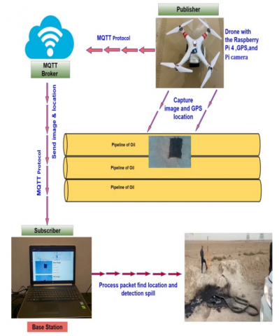
This project uses a drone with a Raspberry Pi, Pi camera, and GPS tracking system to monitor pipelines. MQTT IoT transfers images and location data from the drone to the ground station. Deep learning for computer vision is the foundation. At the base station, the DexiNed technique creates pixel-level thin-edge maps of each image's spill sizes. The LAB approach eliminates shadows since the spill is black. Calculating the contour area using an algorithm may reveal a leak. When a leak is found, the web app sends the original image and the spot's size and position to the authorities. Through the proposed method, solve the problems that other methodologies suffer from, for example, the problem of the secret response to detect and determine the size of the spot, its area, its location, etc.
The remaining sections of the paper are laid out as follows. First, state of the art in related work is presented in Section two. Then, the theoretical underpinnings of the deep learning method employed in this work are presented in Section three. Finally, Section four shows the proposed system design and the obtained result, while conclusions of the work are presented in Section five.
Leak detection has been the major subject of many studies. Wang et al. [7] performed the use of a real-time processing process obtained through video frame monitoring of oil spills, such as midpoint, area, diffusion rate, edge circumference features, etc. They used a recurrent neural network's long-term memory network to find the relationship between features and influencing factors. Li et al. [8] proposed an early micro-leak detection method using a full-coverage three-dimensional capacitance matrix sensor with improved parameters, higher sensitivity, and stable oil leak measurement function. It can detect and quantify small ground tank oil leaks early, ensuring process safety and risk prediction. Wang et al. [9] suggested using an algorithm based on the single flow direction chosen from the 8 possibilities (SFD8) algorithm to predict the path of leaking contaminants at a low leakage rate to ensure pipeline safety in an emergency. By simulating the fluid dynamics of the pollutant's dynamic diffusion process in a computer.
Aba et al. [10] suggested simulating real-time pipeline monitoring and locating damage with an Internet of Things (IoT) analytics platform service. Pressure pulsations monitor pipelines using pipe vibration. Archana et al. [11] proposed machine learning (ML) based anomaly detection models have been. Five ML algorithms were used, to develop pipeline leak detection models. The bolster guiding machine algorithm has been proven as an accurate model for leak detection in oil and gas pipelines. Yang et al. [12] suggested a visual molecular dynamics (VMD) convolutional neural network (CNN) model deep learning (DL) based oil and gas pipeline leak detection model with data preprocessing and pattern recognition. Experimental results show that the used model improves more than other models.
Wang et al. [13] proposed to extract oil spill information using an image CNN model from synthetic aperture radar (SAR) images by taking advantage of its features of local connection, weight sharing, and learning for image representation. Al-Battbootti et al. [14] proposed a framework for computer software that could be used to locate oil spills and river pollution. An unmanned aerial vehicle was used by the artificial intelligence-based framework to locate and identify oil pollution by analyzing the images it had taken. Ali et al. [15] corrosion is one of the faults that have a major influence on the safety of the surface of oil and gas tanks, thus a localizing visual inspection technology combining drones and artificial intelligence (AI) has been presented. This technology employs an image processing algorithm, a fuzzy logic algorithm, and a threshold algorithm. Table 1 shows a summary of related work.
Table 1. Summary of related work
|
Ref. |
Detection Method |
Category |
Technology |
Tools |
Algorithm |
|
[7] |
Video frame monitoring of oil spill handling. |
Exterior |
Analyze the characteristics of the spilled oil. |
CNN |
Long short-term memory network. |
|
[8] |
Sensors |
Exterior |
Full coverage three-dimensional capacitance array sensor. |
Sensors |
Statistical analysis. |
|
[9] |
Predict the path of leaking contaminant. |
Exterior |
Standard Volume of Fluid technique. |
Sensors |
Proposing a Multi-Flow Direction algorithm based on the SFD8 algorithm. |
|
[10] |
Pressure pulses. |
Interior |
Pressure pulses are based on the principle of vibration. |
Arduino UNO R3, Wi-Fi module, and ThingSpeak IoT |
IoT analytics platform service. |
|
[11] |
Anomaly Detection Model. |
Interior |
ML |
Operational parameters temperature, pressure, and flow rate. |
Random forest, support vector machine, k-nearest neighbor, gradient boosting, and decision tree. |
|
[12] |
VMD-MD-1DCNN model. |
Interior |
DL |
Acoustic, pressure, and flow sensors. |
One-dimensional convolution neural network. |
|
[13] |
Sensing image remote to an oil spill. |
Visual |
SAR monitoring of marine oil spills. |
CNN |
AlexNet model |
|
[14] |
Analyze captured images of rivers. |
Visual |
CNN model |
Drones, camera, and Macbook Pro laptop. |
ML.NET |
|
[15] |
Research is to detect rust in oil tanks. |
Visual |
Using AI to localize visual inspection technology through drones. |
drones |
Threshold algorithm, image processing algorithm, and fuzzy logic algorithm. |
|
Our propose work |
Pipeline monitoring using computer vision. |
Visual |
DL algorithm. |
Drone, Raspberry Pi, Pi camera, and GPS. |
DexiNed, LAB algorithm, Spot area calculation algorithm, and MQTT IoT Protocol. |
External detection methodologies are characterized by a set of advantages, for example, they are easy to use, the response time is early, and others and they also have many disadvantages, including the need for highly experienced workers to install and program them, the need for direct contact with the spill medium, the high cost of implementation, the large number of false alarms, and others [16]. As for the internal detection methodologies, they are portable, low cost, and have good performance in implementation, detecting small leaks and the ability to locate them, etc. At the same time, they have a number of defects, including computationally complex to a high degree, and require experts for implementation, and others as for the visual methods, they are considered traditional methods in use, and the difficulty of implementing them in many areas, but they are suitable in a very small area [17].
The field of edge detection has seen widespread implementation across a wide range of practical needs, from the medical to the industrial. It is possible to classify edge detection methods as either traditional edge detection or those based on deep learning [18]. Both the Holistically-Nested Edge Detection (HED) and Xception networks served as bases for DexiNed. Produces human-perceivable narrow edge maps, which may be utilized in any edge detection job without fine-tuning or training [19].
3.1 DexiNed architecture
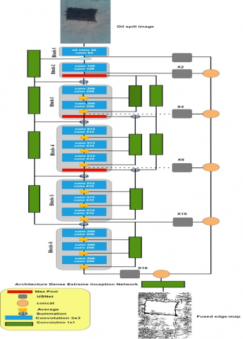
DexiNed is a deep neural network designed to detect edges in BGR images, with inputs represented by W rows and H columns. DexiNed generates six side outputs with different scales, corresponding to edge maps that form an H x W map with values ranging between zero and one, typically mapped to (0, 255) to indicate the presence of edges in the image. Each of the six blocks in DexiNed contributes to the calculation of two main outputs: the average output and the fused output. The fused output is produced by a convolutional layer with a 1×1 kernel, taking the six side outputs as inputs. On the other hand, the average output is computed by averaging all the side outputs and the fused output.
The DexiNed network comprises six blocks, each consisting of repeated sub-blocks. The first block receives a BGR image as input, and its sub-blocks include a convolutional layer with a 3×3 kernel, ReLU activation functions, and batch normalization.
There are some differences in the composition of the six blocks, especially the first and second blocks. These blocks are completely different from the rest of the other four blocks in terms of the presence or absence of ReLU layers before the up-sampling blocks. There are lateral connections, and the 1×1 kernel convolutional layers produce all the lateral connections. The six blocks operate at different scales. The first and second blocks of the input image operate at half-full resolution. In contrast, the third block operates at 1/4 accuracy, the fourth at 1/8 accuracy, and the fifth at 1/16 accuracy. The reduction in precision is achieved through max pooling operations with 2×2 strides and 2×2 kernels.
The architecture of each block varies in terms of the number of convolutional layers and filters. The first block consists of two convolutional layers with 32 and 64 filters each, the second block has two convolutional layers with 128 filters each, the third block has four convolutional layers with 256 filters each, the fourth and fifth blocks have six convolutional layers with 512 filters each, and the sixth block has convolutional layers with 256 filters each.
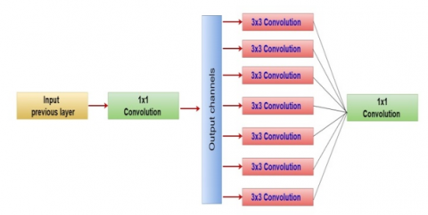
In each block and at different stages, the processed image or its average, in some cases, is added to the output of a side connection. This process is inspired by the Xception network, which uses different layers of pointwise and depthwise convolutions to separate cross-channel connections from spatial connections. Unlike DexiNed, Xception does not utilize the main idea of spatial or cross-channel separation, as it uses standard convolutional layers. Figure 1 illustrates the Dexi architecture [20, 21].
Figure 1. DexiNed architecture [20]
3.1.1 Upsampling architecture
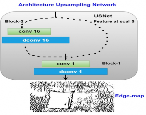
One of the main elements in the DexiNed architecture is the upsampling block (UB), which upscales the edges. The outputs from all DexiNed blocks are inputs to an upsampling block consisting of stacked conditional sub-blocks. Each building block comprises a convolutional and a deconvolutional layer. Figure 2 shows the upsampling network architecture. In the six blocks, the output is upscaled to obtain the full fidelity of the input image. This is done by a set of 1×1 convolution kernels, a ReLU activation function, and 2×2 convolution kernels. Each block specifies the required number of phases. The side outputs of the six blocks are combined by a 1×1 kernel convolution layer to extract an edge map called a fused output. The averaged outputs are obtained by calculating the combined output with the six side outputs, where the sigmoid activation functions are used in all outputs, where the output is in [0, 1], that is, for visualization in a standard form that can be a normalization on [0, 255], and where the edges in the produced image are in color Black and white background [22].
Figure 2. Upsampling network architecture [22]
3.1.2 Loss functions
It is possible to express DexiNed in terms of a regression function ð, that is, $\widehat{Y}$ = ð(X, Y ), where X is an input image, Y is the corresponding ground truth, and $\widehat{Y}$ It is a collection of predicted edge mappings. $\widehat{Y}=\left[\hat{y}_1, \hat{y}_2, \ldots, \hat{y}_N\right]$, where $\hat{y}_i$ has the same size as Y and is the number of outputs from each upsampling block; $\hat{\mathrm{y}}_{\mathrm{N}}$ is the result from the final fusion layer f ($\hat{y}_N=\hat{y}_f$). Therefore, as this is a model, the same loss as (weighted cross-entropy) is used; hence, this problem is thoroughly supervised and addressed similarly.
$\imath^{\mathrm{n}}\left(\mathrm{W}, \mathrm{w}^{\mathrm{n}}\right)=-\beta \sum_{\mathrm{j} \in Y^{+}} \log \sigma\left(\mathrm{y}_{\mathrm{j}} 1 \mid \mathrm{X} ; \mathrm{W}, \mathrm{w}^{\mathrm{n}}\right)$$-(1-\beta) \sum_{j \in Y^{-}} \log \sigma\left(y_j=0 \mid X ; W, w^n\right)$, (1)
Then,
$\mathcal{L}(\mathrm{W}, \mathrm{w})=\sum_{\mathrm{n}=1}^{\mathrm{N}} \delta^{\mathrm{n}} * \imath^{\mathrm{n}}\left(\mathrm{W}, \mathrm{w}^{\mathrm{n}}\right)$, (2)
Each scale has its weight, denoted as, where W is the set of all network parameters and w is the parameter with index, δ is a weight for each scale level. $\beta=\left|Y^{-}\right| /\left|Y^{+}+Y^{-}\right|$ and $(1-\beta)=\left|Y^{+}\right| /\left|Y^{+}+Y^{-}\right|\left(\left|Y^{-}\right|,\left|Y^{+}\right|\right.$ represent the edge and non-edge in the underlying truth, respectively) [23].
3.2 Extreme inception networks
3.2.1 Inception module
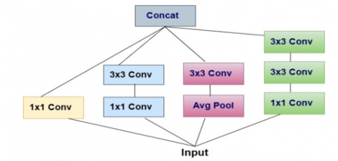
As a bridge between standard convolution and the depthwise separable convolution operation, Inception modules in convolutional neural networks provide an intermediary phase in the learning process (a depthwise convolution followed by a pointwise convolution). In this context, an Inception module with the largest possible number of towers may be seen as a depthwise separable convolution. Several variations on the central "Inception module" form the basis of "Inception-style" models. The standard Inception module, as shown in the Inception V3 design, is depicted in Figure 3. These building blocks are the building blocks of an Inception model.
The first visual geometry group (VGG) style networks were just stacks of basic convolution layers, which is a big change. Although Inception modules and convolutions (convolutional feature extractors) share a lot of common ground, in practice, the former seems able to learn more complex representations with fewer parameters. One convolution kernel, for instance, is responsible for mapping both cross-channel correlations and spatial correlations as a convolution layer seeks to learn filters in a three-dimensional space consisting of two spatial dimensions (width and height) and a channel dimension. The Inception module aims to facilitate this procedure and increase its efficacy by separating it into procedures that may examine cross-channel and spatial correlations separately.
Figure 3. Standard Inception module (Inception V3) [24]
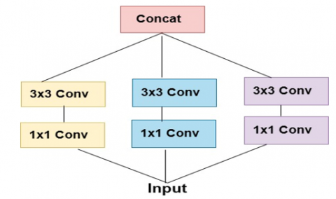
Figure 4. Inception framework simplification [24]
Figure 5. Block diagram of Xception [24]
A stripped-down Inception module that employs just a single convolution size (such as 3×3) and lacks the average pooling tower Figure 3. Figure 4 shows how this Inception module may be reformed as a series of spatial convolutions operating on non-overlapping regions of the output channels. This motivates us to suggest a new kind of deep convolutional neural network design, with depthwise separable convolutions for the Inception modules, named Xception, shown in Figure 5, in the architectural scheme [24].
3.2.2 Xception architecture
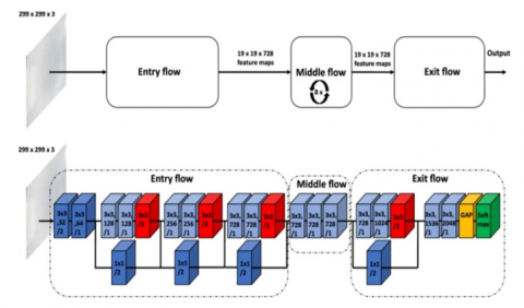
The foundation of a convolutional neural network is a series of convolution layers that may be independently explored in detail [25]. Several of the convolutional layers in its design are responsible for the network's feature extraction mechanism. All modules in the convolutional layers, excluding the first and final, are part of a sum of modules with linear residual connections. Figure 6 depicts the network topology, which consists of three distinct flows. The entry flow begins with extracting coarse features from the input data, then moves to batch normalization and the RELU activation function. In the subsequent middle flow, performed four times, more filters extract more detailed information. As in the VGG-16 architecture, all convolutional layers that may be separated do not undergo depth expansion [26].
Figure 6. Xception CNN architecture [26]
3.3 Holistically-nested edge detection
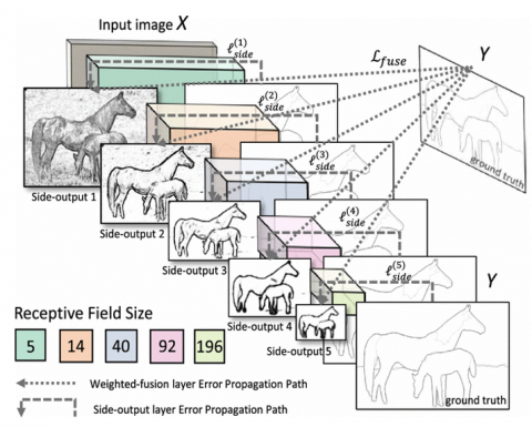
HED employs a VGG16-based deep neural network with additional layers added to combine findings across scales. A color image (three channels) is used as input, and a map with confidence scores between 0 and 1 is produced, where 1 indicates 100% certainty that a given pixel represents an edge. The range of allowed RGB values for each input pixel is [0, 255]. Figure 7 depicts an edge detection network design, with the error backpropagation channels highlighted for clarity. The VGG16 network's convolutional layer is used in this technique. There are 13 convolutional layers, each with a 3×3 kernel and ReLU activation functions. After each layer, the resolution is decreased from one group to the next using a max-pool operation with a 2×2 kernel and a 2×2 stride. The final result of HED combines the outputs of five VGG16 groups trained to represent edge maps at five distinct scales [27].
The HED algorithm is a neural network that takes on two major challenges in long-term vision. Image-to-image prediction using a deep learning model that uses fully convolutional neural networks and deeply-supervised nets is the first step toward a unified image training and prediction approach (the system accepts an image as input and outputs the edge map image) and second, multi-scale and multi-level feature learning motivated by deep neural networks. The complex ambiguity in edge and object boundary detection is resolved by HED's automated learning of rich hierarchical representations (led by deep supervision on side replies) [28].
During training, the input training data set is represented as $\mathrm{S}=\left\{\left(\mathrm{X}_{\mathrm{n}}, \mathrm{Y}_{\mathrm{n}}\right), \mathrm{n}=1, \ldots, \mathrm{N}\right\}$ where sample $X_n=\left\{x_j^{(n)}, j=1, \ldots,\left|X_n\right|\right\}$ represents the raw input image and $Y_n=\left\{y_j^{(n)}, j, \ldots,\left|X_n\right|\right\} y_j^{(n)} \in\{0,1\}$ represents the matching ground truth binary edge map for the image $X_n$. Weights are represented as $\mathrm{w}=\mathrm{w}^{(1)}, \ldots, \mathrm{w}^{(\mathrm{M})}$, and the network comprises M side-output layers. Computes the loss function at the image level for auxiliary outputs. In the field of image-to-image training by [29]:
$\ell_{\text {side }}^{(m)}\left(W, w^{(m)}\right)$$=-\beta \sum_{j \varepsilon Y_{+}} \log \operatorname{Pr}\left(y_j=1 \mid X ; W, w^{(m)}\right)$$-(1-\beta) \sum_{j \varepsilon Y_{-}} \log \operatorname{Pr}\left(y_j=0 \mid X ; W, w^{(m)}\right)$ (3)
Can determine fusion layer loss function $\mathcal{L}_{\text {fuse }}$ By:
$\mathcal{L}_{\text {fuse }}(\mathrm{W}, \mathrm{w}, \mathrm{h})=\operatorname{Dist}\left(\mathrm{Y}, \hat{\mathrm{Y}}_{\text {fuse }}\right)$ (4)
To optimize for the minimum value of the following objective function using (backpropagation) accidental fall down a gradient by:
$(\mathrm{W}, \mathrm{w}, \mathrm{h})^*=\operatorname{argmin} \mathcal{L}_{\text {side }}(W, w)+\mathcal{L}_{\text {fuse }}(W, w, h)$ (5)
Both the side output layers and the weighted-fusion layer's predictions on the edge map may be used in the testing step with image X by:
$\hat{Y}_{\text {fuse }}, \hat{Y}_{\text {side }}^{(1)}, \ldots, \hat{Y}_{\text {side }}^{(\mathrm{M})}=\operatorname{CNN}\left(X,(\mathrm{~W}, \mathrm{w}, \mathrm{h})^*\right)$ (6)
These created edge maps may be aggregated further to provide a single result by:
$\hat{Y}_{H E D}=\operatorname{Average}\left(\hat{Y}_{\text {fuse }}, \hat{Y}_{\text {side }}^{(1)}, \ldots, \quad \hat{Y}_{\text {side }}^{(\mathrm{M})}\right)$ (7)
Figure 7. Network architecture for HED [27]
3.4 LAB color space
A luminance (lightness) channel, and two additional channels, A and B, represent different chromaticity layers in this color space. Where a color lies on the red-green axis can be determined from the A* layer, and where it lies on the blue-yellow axis may be selected from the B* layer. The fact that this color space may convey color information across multiple platforms and devices is its most notable characteristic. Coordinates in L*A*B* color space, the range of possible values for L* is from 0 (complete darkness) to 100 (total lightness) brightness (L*) is displayed along the middle vertical axis. It follows from the coordinate axes that A* color can't be blue or yellow since these are opposing colors [30].
All axes display values from positive to negative. The A channel, whose values range from -128 to +127, reveals the color balance between red and green. The B channel, whose values range from -128 to +127, also specifies the image's relative amount of yellow and blue. Colors with a high value in the A or B channels tend to be red or yellow. In contrast, colors with a low value tend to be green or blue. The zero point shows grayscale neutrality on both axes.
An image with RGB is converted to a LAB image by converting it to grayscale images or binary images. This is done to detect edge information in the image. The space RGB is converted to space XYZ and then converted to space LAB. The value range is R, G, and B=(0 $\sim$ 255), L=(0 $\sim$ 100), and A, B=(-128 $\sim$ +128). The color values of R, G, and B are converted to X, Y, and Z by Eq. (8) [31].
$\left\{\begin{array}{c}X=0.49 \times R+0.31 \times G+0.2 \times B; \\ Y=0.177 \times R+0.812 \times G+0.011 B; \\ Z=0.01 \times G+0.99 \times B.\end{array}\right.$ (8)
The values X, Y, and Z are converted into LAB using Eq. (9):
$\left\{\begin{array}{c}L=116 f_Y-16 ; \\ A=500 \times\left(\frac{f_X}{0.982-f_Y}\right) ;\\ B=200 \times\left(f_Y-\frac{f_Z}{1.183}\right).\end{array}\right.$ (9)
Leakage detection systems for underground crude oil pipelines must meet a number of criteria, the most essential of which is the ability to detect spills of varying sizes. The age of the pipe, environmental degradation, vandalism, and theft are all potential reasons for a leak. Slow leaking might cause the size of the spill to grow over time. Second, the color of the spill itself, which is always dark owing to the oil's composition. The color of the spill does not fade over time.
The location of the leak is the last criterion in the design process. The majority of leak detection systems, such as differential pressure, may identify a leak in a certain section of pipe (up to 30 km), but they cannot pinpoint its precise position within that segment. Part of the system's implementation is seen in Figure 8, and the actions involved may be summed up as follows:
4.1 Experimental work
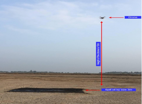
This work employed an embedded system using a drone (DJI- Phantom 3 Advanced model. The battery life is 23 minutes with the autopilot feature. It rises vertically at a speed of up to 13 km/h while flying horizontally at a speed of up to 35 kilometers/hour. The aircraft weighs approximately 453 grams as it is equipped with sensing technology in the presence of heights in front of it to avoid a collision), represented by a Raspberry Pi 4, equipped with a Raspberry Pi v2 camera module and a NEO-6M GPS module, to determine the volume and position of a spill anywhere along the pipelines. A drone is given the coordinates of the pipeline routes and deployed on a tour, during which it carries the embedded system. The architecture and execution of the suggested system are shown in Figure 9.
Figure 8. Drone taking images of the oil leakage
Figure 9. Proposed system design and implementation
A drone is regularly launched down a conduit that is approximately three meters underneath. The method was put through its paces on a 30-kilometer oil pipeline in the Iraqi desert. per 0.2 seconds, the embedded device snaps an image at a set position along the route, capturing an image per meter. Using the MQTT IoT protocol, the image is sent to the base station along with its GPS coordinates. DexiNed is an image analysis method that looks for sharp edges and corners. A spill might be one of the numerous possible forms in any given image. Therefore, minor contour details would be ignored. Then, the LAB method is used to locate the edge of an image with a single black color spot, a possible spill.
4.2 Base station design
The suggested web app has been built to operate as a hub that receives data packets from the drone through the MQTT protocol, with the drone playing the role of publisher and the web app taking on the role of the subscriber. The first thing that happens is that the program gets images with its GPS coordinates (longitude and latitude). The site then uses separate algorithms to analyze the data and make a determination on the spill after getting this information. Python 3.9 with the Flask framework and a Microsoft Access database power this app. In this study, have developed three algorithms:
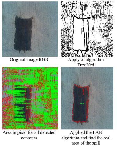
The first algorithm depicts the publish/subscribe schema used by the MQTT IoT Protocol, with the drone and Raspberry Pi 4 playing the role of publishers and the base station the role of subscribers. Applying the DexiNed deep learning algorithm to the incoming images, determining the contour for all image parameters, and erasing the smallest contour below the threshold limit are all steps in the second method. Finally, the third algorithm uses the LAB algorithm to find contours with only black features (the natural color of the spill), and then either sends a warning via the web application of the spill's location if the spot area is larger than the threshold limit, or stores the information in the database at the present time and checks it in the next round of the drone. The final product of the image processing is shown in Figure 10.
Figure 10. 3m2 spill with 10 m height
|
Algorithm1: MQTT IoT Protocol |
|
|
1 |
The base station sends the message to the drone to start the operation. |
|
2 |
{ |
|
3 |
While (True): { |
|
4 |
Image=capture (image_ path) |
|
5 |
[latitude, longitude]=read GPS location |
|
6 |
Payload message =image+ latitude+ longitude |
|
7 |
Publish (Payload) to Base Station |
|
8 |
} |
|
9 |
} |
|
Algorithm 2: Apply DexiNed |
||
|
1 |
Read image |
|
|
2 |
Apply DexiNed |
|
|
3 |
Number of contours =n; |
|
|
4 |
{ |
|
|
5 |
While (n!=0) { |
|
|
6 |
If contour _ area _ in pixel(small) |
|
|
7 |
{ |
|
|
8 |
Eliminate contour; |
|
|
9 |
n--; |
|
|
10 |
} |
|
|
11 |
Else { |
|
|
12 |
Contour _ counts++; |
|
|
13 |
n--; |
|
|
14 |
} |
|
|
15 |
} |
|
|
16 |
} |
|
|
Algorithm 3: LAB Algorithm |
||
|
1 |
Read image i from DexiNed. |
|
|
2 |
While (True): |
|
|
3 |
{ |
|
|
4 |
Apply the LAB algorithm. |
|
|
5 |
If (black _ contour) exists |
|
|
|
If (area _ black_contour> threshold) |
|
|
6 |
{ |
|
|
|
Send an alarm message to find leakage by a web application. |
|
|
7 |
Set a new round. |
|
|
8 |
} |
|
|
|
Else |
|
|
9 |
{ |
|
|
|
Save the image in a database. |
|
|
10 |
} |
|
|
11 |
Else |
|
|
12 |
{ |
|
|
13 |
Check the database for the stored image. |
|
|
14 |
If the spill exit in a database |
|
|
15 |
{ |
|
|
16 |
Get the GPS location of the spill. |
|
|
17 |
Send the drone to a location. |
|
|
18 |
} |
|
|
19 |
Else |
|
|
20 |
{ |
|
|
21 |
Set a new round. |
|
|
22 |
} |
|
|
23 |
} |
|
|
24 |
}
|
|
4.3 Area calibration procedure
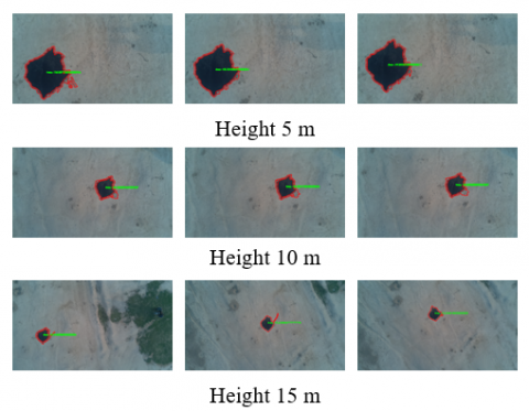
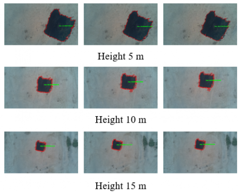
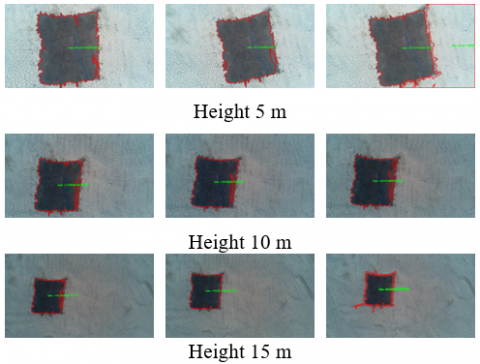
Extensive testing was conducted in this study, where three sizes of the spill were done (1m2, 2m2, and 3m2), to calculate the real area of the spill, as shown in Figure 11. For each area size, the drone is positioned immediately above the spill at one of three heights (5m, 10m, and 15m). Up to ten images were taken for each peak as in Figure 11. The images used to calculate the spill area in pixels and the spill diameter are summarized statistically in Table 2.
Table 2. Statistical analysis of a group of images captured in pixels
|
Image |
Pixel Area |
Perimeter Area |
|
Height=5 and the Spill is 1m2 |
||
|
1 |
101204.5 |
2478.83 |
|
2 |
97713.5 |
1816.19 |
|
3 |
96422.0 |
1568.59 |
|
4 |
87357.0 |
1384.76 |
|
5 |
91652.0 |
1373.94 |
|
Height=10 and the Spill is 1m2 |
||
|
1 |
23219.0 |
725.41 |
|
2 |
23019.5 |
797.25 |
|
3 |
23103.5 |
814.28 |
|
4 |
23099.0 |
762.38 |
|
5 |
23122.0 |
792.52 |
|
Height=15 and the Spill is 1m2 |
||
|
1 |
8078.0 |
457.1 |
|
2 |
7610.5 |
363.12 |
|
3 |
8760.0 |
499.16 |
|
4 |
8342.0 |
431.91 |
|
5 |
8041.0 |
393.42 |
|
Height=5 and the Spill is 2m2 |
||
|
1 |
158437.0 |
2032.64 |
|
2 |
153535.0 |
2030.09 |
|
3 |
158332.5 |
2015.99 |
|
4 |
184341.0 |
2309.71 |
|
5 |
162207.5 |
2083.99 |
|
Height=10 and the Spill is 2m2 |
||
|
1 |
61926.0 |
1170.63 |
|
2 |
63696.0 |
1396.94 |
|
3 |
64244.5 |
1311.79 |
|
4 |
60996.5 |
1245.02 |
|
5 |
59781.5 |
1230.73 |
|
Height=15 and the Spill is 2m2 |
||
|
1 |
27382.5 |
767.71 |
|
2 |
27901.0 |
753.47 |
|
3 |
27481.0 |
711.04 |
|
4 |
27127.0 |
703.39 |
|
5 |
25840.0 |
864.1 |
|
Height=5 and the Spill is 3m2 |
||
|
1 |
259915.0 |
2758.26 |
|
2 |
254728.0 |
2932.97 |
|
3 |
254765.0 |
3213.02 |
|
4 |
251951.0 |
3627.29 |
|
5 |
261107.5 |
3273.14 |
|
Height=10 and the Spill is 3m2 |
||
|
1 |
143821.0 |
2523.32 |
|
2 |
138306.5 |
1932.6 |
|
3 |
135590.5 |
2400.83 |
|
4 |
138213.0 |
2475.24 |
|
5 |
138131.5 |
2364.26 |
|
Height=15 and the Spill is 3m2 |
||
|
1 |
68020.5 |
1916.86 |
|
2 |
62248.0 |
1232.75 |
|
3 |
61547.5 |
1240.65 |
|
4 |
62929.5 |
1296.65 |
|
5 |
63246.5 |
1229.6 |
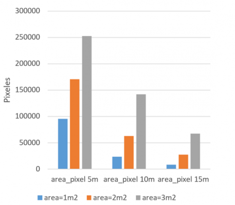
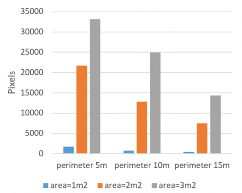
By using the DexiNed deep learning technique, identified the spill, which might lead to several contours, a large spill contour, or even very tiny contours. There must be an algorithm to get rid of the contours and separate the oil slick by color from the rest of the slicks. The comparison of the pixel area to the perimeter of the three spills at the three heights is shown in Figures 12 and 13. A rough estimate of the area may be made from the pixel area, allowing for the simple calculation of the perimeter, whether it be tiny or vast.
(a) 1m2 area of the leakage
(b) 2m2 area of the leakage
(c) 3m2 area of the leakage
Figure 11. Image of spilled oil of different sizes taken by a drone
Figure 12. Average pixel area of a set of leakage images
Figure 13. The average perimeter of a set of leakage images
4.4 Web application
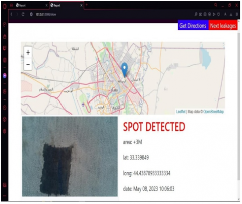
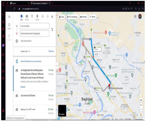
During the first flight, the MQTT IoT protocol is used to transmit data from the drone to a server, where it is processed and presented online. If one of the images has a spot and the contour area is two meters or more, it is considered a leak, and the details appear, including a map showing the location and spill information (volume of the spill, location of the spill, date when the spill was seen, and area of spill), as shown in Figure 14. The geographic distance from the hub station to the observation site is shown in Figure 15.
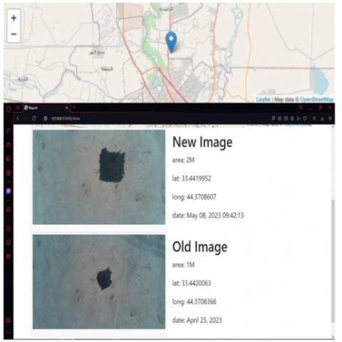
But if the spot contour area is smaller than the minimum (1m2), it is not deemed a leak, and the image with its position is preserved in the database to monitor it. It will be shown in the Figure 16 with the first scenario before it is regarded as a leak if the spot perimeter area is larger than the threshold limit in further rounds of the drone compared to the stored spot size and position. Displaying all detected images and pre-processed oil spill suspects allows the system to provide a summary of each round the drone does.
Figure 14. The main interface of the program for the presence of an oil spill is greater than the threshold limit
Figure 15. Distance between the spill and the main station
Figure 16. Main program interface for an oil spill expansion
This work proposes the development and assessment of a computer vision and image processing monitoring system, using deep learning techniques and drones. Using the DexiNed algorithm, which was validated by statistical comparison to other edge detection methods using basic metrics (per-image best threshold (OIS)=0.867, fixed contour threshold (ODS)=0.859, and average precision (AP)=0.905), thin edge maps were generated, with oil slick identification included. The LAB algorithm has been validated for its ability to reliably detect black spills, calculate spill area, and establish whether or not it is excessive. When comparing findings from different altitudes, 10 meters was the best height for the airplane, which gives a good view of the image. Therefore, the proposed method could enrich this stream type of research through an automated process with intelligent decision-making. Works like [13-15] are close to this work in some features. The proposed work differs from them by using the powerful edge detection algorithm DexiNed and a drone which is a provided mobile camera rather than the fixed one. The fixed camera is not an appropriate approach for a wide area and long pips which could reach hundreds of kilometers like the case in Iraq (the case study in this work).
However, the functioning of the system is hindered by a few elements, such as the weather conditions during the inspection rounds and the fact that the precision of the image varies with the time of day and the terrain over which the pipes traverse. can use the drone network (Internet of drones) to check the overall national pipes network.
Iraqi Commission supports this work for Computers and Informatics /Informatics Institute for Postgraduate Studies.
[1] Wang, Q.Y., Song, Y.H., Zhang, X.S., Dong, L.J., Xi, Y.C., Zeng, D.Z., Liu, Q.L., Zhang, H.L., Zhang, Z., Yan, R., Luo, H. (2023). Evolution of corrosion prediction models for oil and gas pipelines: From empirical-driven to data-driven. Engineering Failure Analysis, 146: 107097. https://doi.org/10.1016/j.engfailanal.2023.107097
[2] Jasim, F.M., Al-Isawi, M.M.A., Hamad, A.H. (2022). Guidance the wall painting robot based on a vision system. Journal Européen des Systèmes Automatisés, 55(6): 793-802. https://doi.org/10.18280/jesa.550612
[3] Hamad, A.H., Fadhil, H.M. (2022). Appraisal of intelligent notification system for smart university campus based internet of objects for social activities. AIP Conference Proceedings. 2386(1): 050006. https://doi.org/10.1063/5.0066789
[4] Korlapati, N.V.S., Khan, F., Noor, Q., Mirza, S., Vaddiraju, S. (2022). Review and analysis of pipeline leak detection methods. Journal of Pipeline Science and Engineering, 2(4): 100074. https://doi.org/10.1016/j.jpse.2022.100074
[5] Marathe, S. (2019). Leveraging drone-based imaging technology for pipeline and RoU monitoring survey. Paper presented at the SPE Symposium: Asia Pacific Health, Safety, Security, Environment and Social Responsibility, Kuala Lumpur, Malaysia. https://doi.org/10.2118/195427-ms
[6] Ibraheem, S.S., Hamad, A.H., Abdulhadi Jalal, A.S. (2018). A secure messaging for Internet of Things protocol based RSA and DNA computing for video surveillance system. In 2018 Third Scientific Conference of Electrical Engineering (SCEE), Baghdad, Iraq, pp. 280-284. https://doi.org/10.1109/SCEE.2018.8684055
[7] Wang, R., Zhu, Z., Zhu, W., Fu, X., Xing, S. (2021). A dynamic marine oil spill prediction model based on deep learning. Journal of Coastal Research, 37(4): 716-725. https://doi.org/10.2112/JCOASTRES-D-20-00080.1
[8] Li, L., Chen, H., Huang, Y., Xu, G., Zhang, P. (2022). A new small leakage detection method based on capacitance array sensor for underground oil tank. Process Safety and Environmental Protection, 159: 616-624. https://doi.org/10.1016/j.psep.2022.01.020
[9] Wang, K., Peng, J., Zhao, J., Hu, B. (2022). Analysis of leaked crude oil in a mountainous area. Energies, 15(18): 6568. https://doi.org/10.3390/en15186568
[10] Aba, E.N., Olugboji, O.A., Nasir, A., Olutoye, M.A., Adedipe, O. (2021). Petroleum pipeline monitoring using an Internet of Things (IoT) platform. SN Applied Sciences, 3: 1-12. https://doi.org/10.1007/s42452-021-04225-z
[11] Archana, V., Kalaiselvi, S., Thamaraiselvi, D., Gomathi, V., Sowmiya, R. (2022). A novel object detection framework using Convolutional Neural Networks (CNN) and RetinaNet. In 2022 International Conference on Automation, Computing and Renewable Systems (ICACRS), pp. 1070-1074. https://doi.org/10.1109/ICACRS55517.2022.10029062
[12] Yang, D., Lu, J., Zhou, Y., Dong, H. (2022). Establishment of leakage detection model for oil and gas pipeline based on VMD-MD-1DCNN. Engineering Research Express, 4(2): 025051. https://doi.org/10.1088/2631-8695/ac769e
[13] Wang, X., Liu, J., Zhang, S., Deng, Q., Wang, Z., Li, Y., Fan, J. (2021). Detection of oil spill using SAR imagery based on AlexNet model. Computational Intelligence and Neuroscience, 4812979. https://doi.org/10.1155/2021/4812979
[14] Al-Battbootti, M.J.H., Goga, N. Marin, I. (2022) Detection and analysis of oil spill using image processing. International Journal of Advanced Computer Science and Applications, 13(4): 381-387. https://doi.org/10.14569/IJACSA.2022.0130445
[15] Ali, M.A.H., Baggash, M., Rustamov, J., Abdulghafor, R., Abdo, N.A.-D.N., Abdo, M.H.G., Mohammed, T.S., Hasan, A.A., Abdo, A.N. (2023). An automatic visual inspection of oil tanks exterior surface using unmanned aerial vehicle with image processing and cascading fuzzy logic algorithms. Drones, 7(2): 133. https://doi.org/10.3390/drones7020133
[16] Aljuaid, K.G., Albuoderman, M.A., AlAhmadi, E.A., Iqbal, J. (2020). Comparative review of pipelines monitoring and leakage detection techniques. In 2020 2nd International Conference on Computer and Information Sciences (ICCIS), Sakaka, Saudi Arabia, pp. 1-6. https://doi.org/10.1109/ICCIS49240.2020.9257602
[17] Adegboye, M.A., Fung, W.K., Karnik, A. (2019). Recent advances in pipeline monitoring and oil leakage detection technologies: Principles and approaches. Sensors, 19(11): 2548. https://doi.org/10.3390/s19112548
[18] Bakirman, T., Kulavuz, B., Bayram, B. (2023). Use of artificial intelligence toward climate-neutral cultural heritage. Photogrammetric Engineering & Remote Sensing, 89(3): 163-171. https://doi.org/10.14358/PERS.22-00118R2
[19] Portela, H.M.B.F., Veras, R.D.M.S., Vogado, L.H.S., Leite, D., de Sousa, J.A., de Paiva, A.C., Tavares, J.M.R.S. (2022). A coarse to fine corneal ulcer segmentation approach using U-net and DexiNed in chain. In Progress in Pattern Recognition, Image Analysis, Computer Vision, and Applications: 25th Iberoamerican Congress, CIARP 2021, Porto, Portugal, pp. 13-23. https://doi.org/10.1007/978-3-030-93420-0_2
[20] Grompone von Gioi, R., Randall, G. (2022). A brief analysis of the dense extreme inception network for edge detection. Image Processing On Line, 12: 389-403. https://doi.org/10.5201/ipol.2022.423
[21] Soria, X., Riba, E., Sappa, A. (2020). Dense extreme inception network: Towards a robust CNN model for edge detection. In 2020 IEEE Winter Conference on Applications of Computer Vision (WACV), Snowmass, CO, USA, pp. 1912-1921. https://doi.org/10.1109/WACV45572.2020.9093290
[22] Soria, X., Sappa, A., Humanante, P., Akbarinia, A. (2023). Dense extreme inception network for edge detection. Pattern Recognition, 139: 109461. https://doi.org/10.1016/j.patcog.2023.109461
[23] Tian, Z.H., Chen, D.L., Liu, S.X., Liu, F. (2020). DexiNed-based aluminum alloy grain boundary detection algorithm. In 2020 Chinese Control and Decision Conference (CCDC), Hefei, China, pp. 5647-5652. https://doi.org/10.1109/CCDC49329.2020.9164634
[24] Chollet, F. (2017). Xception: Deep learning with depthwise separable convolutions. In 2017 IEEE Conference on Computer Vision and Pattern Recognition (CVPR), Honolulu, HI, USA, pp. 1800-1807. https://doi.org/10.1109/CVPR.2017.195
[25] Brodzicki, A., Piekarski, M., Kucharski, D., Jaworek-Korjakowska, J., Gorgon, M. (2020). Transfer learning methods as a new approach in computer vision tasks with small datasets. Foundations of Computing and Decision Sciences, 45(3): 179-193. https://doi.org/10.2478/fcds-2020-0010
[26] Raksarikorn, T., Kangkachit, T. (2018). Facial expression classification using deep extreme inception networks. In 2018 15th International Joint Conference on Computer Science and Software Engineering (JCSSE), Nakhonpathom, Thailand, pp. 1-5. https://doi.org/10.1109/JCSSE.2018.8457396
[27] von Gioi, R.G., Randall, G. (2022). A brief analysis of the holistically-nested edge detector. Image Process. Line, 12: 369-377. https://doi.org/10.5201/ipol.2022.422
[28] Yu, N.G., Zhang, Z., Xu, Q., Firdaous, E., Lin, J. (2021). An improved method for cloth pattern cutting based on holistically-nested edge detection. In 2021 IEEE 10th Data-Driven Control and Learning Systems Conference (DDCLS), Suzhou, China, pp. 1246-1251. https://doi.org/10.1109/DDCLS52934.2021.9455545
[29] Xie, S.N., Tu, Z.W. (2017). Holistically-nested edge detection. International Journal of Computer Vision, 125(1-3): 3-18. https://doi.org/10.1007/s11263-017-1004-z
[30] Dong, L.L., Zhang, W.D., Xu, W.H. (2022). Underwater image enhancement via integrated RGB and LAB color models. Signal Processing: Image Communication, 104: 116684. https://doi.org/10.1016/j.image.2022.116684
[31] El Abbadi, N.K., Saleem, E. (2020). Automatic gray images colorization based on lab color space. Indonesian Journal of Electrical Engineering and Computer Science, 18(3): 1501-1509. https://doi.org/10.11591/ijeecs.v18.i3.pp1501-1509