Assad Al-Shueli*![]() | I. A. Al-Tahar
| I. A. Al-Tahar![]()
© 2023 IIETA. This article is published by IIETA and is licensed under the CC BY 4.0 license (http://creativecommons.org/licenses/by/4.0/).
OPEN ACCESS
In clinical applications and studies neural nerve impulse recordings are extensively used. The spike detection method is critical for determining when a spike is activated. The minimal ratio of signal to noise for multi-electrode cuff recordings is generally less than 10. For applications involving implantable neural recording, this work provides a brand-new, incredibly hardware-efficient (low complexity, low computation), adaptive spike detection algorithm. A mean reduction filter is used in this to first remove any low-frequency elements from the data without adding more phase distortion. A new operator called an Amplitude Slope Operator (ASO) is also added as a hardware-effective substitute for NEO for increasing the SNR of the data. The adjustable threshold is computed on a periodic basis by subtracting any detected spikes from the running mean while simultaneously running a subthreshold detection to remove some of the undetected spikes from the background activity. The method was first created in Matlab employing floating-point math, and it has since been converted to work with fixed-point math. The Least mean squares (LMS) adaptive filter is proposed and implemented in this research using Matlab and the Xilinx Spartans 3E-100 (xc3s100e) hardware and software tools. The proposed filter improves noise rejection while also reducing power consumption and hardware footprint. Furthermore, the results show that its LMS adaptive filter works effectively in online neural recording, with significant improvements in the signal-to-noise ratio (SNR). As a result, this enhancement may result in greater spike detection accuracy. In records with SNR = 5, it can achieve a sensitive of >80% with such a false-positive rate of 6 Hz, and it improves performance than an optimum threshold detector employing a band - pass filter in records with SNR > 3. In comparison to the traditional technique of digital filter algorithm, the current filter design delivers a significant decrease of 10% in power usage and 25% in hardware requirements. As a result, this research might point to a critical advance in brain recording to be used as a control input for prostheses devices.
neural recordings, LMS adaptive filter noise elimination, spike detection. FPGA
Humans have long been interested in the possibilities of regulating prostheses using non natural or bio-natural impulses, which has prompted researchers as manufacturers to do more study in this sector, such as intelligent prosthesis and function electromyography (EMG) [1-3]. Spike recordings using multi-electrode cuffs (MECs) are primarily determined by the sharpness of a electro-neuro-gram (ENG) data [4-8]. The MECs technique might increase noise rejection for recorded action potential. A less invasive electrode cuff nerve fibre connection approach for recording APs could extract spike data with amplitudes ranging from 1 to 5 Volt peak to peak, a signal to background noise ratio band of 1.2 - 3.8 dB [9], and a signal frequency range of 1 Hz to 3 kHz [10]. The essential feature of velocity selective recordings (VSR) approach is based on MEC interface method and nerve impulse dispersion via nerve fibber, the tripolar-electrode-cuff attached around the specific nerve fibber bundles generates identical signals at the ends of the op - amps, the delay line (T, 2T, 3T, NT) arrange to match to electrodes pitching distance and their travel velocity. The neuronal action potentials obtained are dependent on AP speed and their arbitrary time delays match (N...3...2,) this approach is known as matching velocity [4]. This technique is used for spike magnitude and noise tolerance capabilities are sensitive to aspects such as amplifier layout (unipolar, tripolar, or monopolar), filter characteristic, and amplifier strength.
Several research offer a classic DSP (digital signal processor) for digital filter construction to conduct mathematical operations on signal fully digital magnitudes as well as their major utilisation in producing computer and costume microcontroller [11]. The primary advantages of the DSP approach are processing speed, hardware cost, and the flexibility to execute a specific application using a DSP chip or ASIC (application specific integrated circuits). However, DSP algorithms continue to have limited utility in online recording and are costly. Another technology used is FPGA (Field Programmable Gate Arrays), which combines the properties of both ASIC and DSP. Moreover, the FPGA's capabilities, such as reprogramming and reconfiguring, make the system easier to adapt and deploy. As a result, the adaptable filter is configured using an FPGA board.
New studies [12-15] aims to reduce filter order by decreasing the range of a delay line. However, changing the sequence of the filters does not totally use for memory and power savings in implementing on Xilinx and ASIC systems. Furthermore, reducing filter order may result in lengthy length coefficient values, resulting in an unnecessary increase in hardware size and a significant fall in noise reduction capabilities.
The current study proposes a further decrease in device power and size consumption by utilising the parallelism feature of the Xilinx, without increasing the complexity of the hardware design. Because of advancements in the capability of digital signal processors, adaptive filters are now commonly utilised in devices such as healthcare monitoring equipment.
The key aims of this research are to provide the best LSM adaptive filter method for brain spike signal recording performed on FPGA. MATLAB program 2010, Modelsim (De 6.5e) software, Xilinx (Integrated Software Environment) (ISE) Suite (14.2), and FPGA Spartan (3E-100 xc3s100e) board and laptop were used to create the filter. The MATLAB fixed-point toolbox is used to calculate the LMS digital filter weights, which are then reused to synthesise the system on FPGA alongside the other units for the entire detection process.
The primary advantage of this strategy is that it reduces live time neural recording while conserving device and power resources. Furthermore, the present adaptive filter has also been confirmed and run on an FPGA board with such a non biological signal generator, which was previously done in our work [16].
Figure 1. The whole system structure
2.1 System structure
Figure 1 depicts the entire system units for the LMS adaptive filter. Unit one is made up of a ten-channel synthetic bipolar pulse generator (implemented and characterised in more detail in [16]) that is employed to supply data input for the SPU for the ANN approach unit, that was previously implemented in the previous study [17]. Unit two turned the ten bipolar streams into nine tripolar channels, which were then supplied into the ANN processing block [18-20] for a structure with (N+1) electrodes, there will be (N) bipolar channels and (N-1) tripolar ones. Unit three is the proposed LMS adaptive filter used in this work to increase discriminating recording and noise reduction.
2.2 Adaptive filter technique
The adaptive filter used in a wide range of applications due to the creation of sophisticated adaptive algorithms and the use of powerful digital signal processors. Over the past two decades, adaptive techniques have been successfully used in a vast array of various applications. Numerous configurations could be used in a number of various industries, including radar, sonar, audio and video signal processing, and noise reduction, among others.
The design method and adaptation algorithm are the primary determinants of how effective adaptive filters are. The adaptive filters can have analog designs, digital designs, or mixed designs, each of which has benefits and disadvantages. For instance, analog filters are quick to respond and use little power, but they have offset issues that interfere with the functioning of the adaptation algorithm [20]. The digital filters provide a more precise response and are offset-free. Additionally, the adaptive filters may combine various filter types, such as linear or nonlinear, finite impulse response (FIR) or infinite impulse response (IIR) filters, single-data or multi-input data filters, and linear or nonlinear.
There are several ways available for adaptive filter construction and tuning. Because of these properties and capabilities for working in a real-time environment, a high SNR, low silicon and power usage for this implementation approach is nominated in this study. Furthermore, the present filter design provides great performance and is suitable for neural recording applications.
The filter parameters are adjusted on the basis of reducing the mean squared error (MSE) that exists between the intended signal and the filter output. The two most popular adaptation algorithms are Recursive Least Square (RLS) and Least Mean Square (LMS). RLS provides a faster convergence rate than LMS, but LMS retains its edge in terms of computation complexity. The LMS algorithm is most frequently used in the design and execution of integrated adaptive filters due to its computational simplicity.
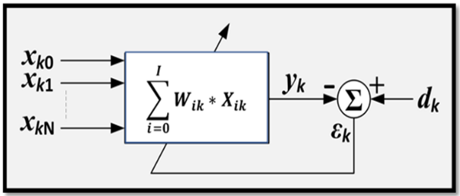
Figure 2. The filter structure of the LMS adaptive procedure
The (LMS) adaptive filter structure shown in Figure 2 is chosen because it outperforms alternative type of digital filter. Moreover, the major benefit of this filter implementation, it necessitates minimal arithmetic complications than some other techniques (such like RLS), and there is no complicated implementation needed in practice. FIR filters having a linear phase, therefore the signal always is steady, which is a huge benefit over IIR filters because FIR filters contain just zeros and are still (BIBO) stable. Signal processing requires a high level of stability.
2.3 LMS procedure
The LSM proposed technique has a sequential delay line identical to the FIR filter configuration as shown in Figure 3; therefore, the model parameters of the LMS adaptive filter must be updated based on the error value of each individual sample, and the adaptive filter weights are tuned as indicated below:
Wi,k+1=win+2µɛk+1, for i=0, 1, …, I (1)
The LMS method is independent of the input data x(n) and therefore does not necessitate any specific connection. As a result, it might be used to tune a linear integrator as well as a FIR filter. In this case, the modified phrase looks like this:
Wi,k +1=wik+2µɛk (2)
The LMS process acts somewhere at each sample, (k), to create a little update in the single coefficient. If the trend of the change is utilised at sample time k, it may lessen the error. The magnitude of the variance in each coefficient is determined by, the amount of the linked x, and the errors at sample (k). The coefficients that have the most impact upon the output stream, (y(k), are modified the most. When the mistake becomes zero, the updating of the coefficient values should be halted. If indeed the associated magnitude of (x) is zero, such that updating the weight creates negligible variance, then no change happens.
The convergence parameter (μ), as indicated in (3), governs algorithm performance and depicts the approach speed and appropriate filter weights. If μ the value is sufficiently large, the strategy will fail to converge. A extremely small value of, in contrast hand, causes the approach to converge slowly and prevents it from following variable states. If (μ) the value is significant but not too big to prevent convergence, the technique quickly obtains a steady-state. The sequins, on the other hand, overshoot the optimum coefficient vector. In certain circumstances, (μ) is initially big for quick convergence and later lowered to reduce overshoot.
However, with proven predictions for stability and uniqueness, the approach converges condition as follows [21, 22]:
$0<\mu<\left[\frac{1}{\left(\sigma^2\right)}\right]$ (3)
where,
$\sigma^2=\sum_{i=0}^I \sigma_i^2$ (4)
δσi equal RMS magnitude of input stream.
In successive FIR filter, every input has an equal RMS magnitude since all the signals are equal, but they are delayed among each other. So, the total power in this circumstance equal to:
$\sigma^2=\left[(L+1) *\left(\sigma_0^2\right)\right]$ (5)
The a normalized LMS approach:
$w_{i, k+1}=w_{i k}+\left[\left(\frac{2 \mu_\sigma}{\sigma^2}\right) \varepsilon_k * x\right]-1$ (6)
The convergence (μ) expression is: $0<\mu<\left[\frac{1}{\sigma^2}\right]$.
2.4 Design of an LMS adaptive filter
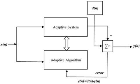
The LSM model design comprises of output computation magnitudes, error, filter learning rate, and cost function. The suggested process consists of four steps. The adaptive approach, as shown in Figure 2, is built on incorrect feedback toward the LMS digital filter weights.
a) Level one:
Calculate the output magnitudes (y(n)) using (7).
$y(n)=\sum_k^{I-1} x(n-k) * w(k)=x_n^t * w_n$ (7)
where,
The model output of LMS adaptive filter = (y(n)), and the Loop Length=I.
The input delay line of the filter sample=x(n-k), and the filter weight=wn(k).
b) Level two:
The error [e(n)] generating from (8).
$e(n)=[d(n)-y(n)]$ (8)
where, Error data=e(n), Desired data=d(n).
c) Level three:
The computation of (β) by locating the variance (σ2) in (9) with the lowest computation cost;
$\begin{aligned} \sigma^2(n)= & {\left[0.95 * \sigma^2(n-1)\right]+\left(\frac{e^2(n)}{n}\right) } \\ & \text { if } n=0 ;\left[\sigma^2(n)\right]=1\end{aligned}$ (9)
where, (β) and (σ2(n)) represent the cost function and variance of the filter model respectively.
d) Level four:
The computation of weights (wn+1(k)) is presented in (10). The LMS model of the adaptive filter weight is adjusted based on the next equation in (10) (wn (k)) and (wn+1 (k)) represents the current and next coefficient values, respectively, the learning rate is represented as (μ) and the input is x(n-k).
$w_{n+1}(k)=w_n(k)+[\mu * \operatorname{sign}[e(n)] * x(n-k)]$;
if $(|e(n)|)>\sigma^2=w_n(k)+\mu *\left[\left(\frac{2}{\sigma^2}\right)-\left[\frac{|e(n)|}{\sigma^2}\right]\right] * e(n) * x(n-k)$;
if $(|e(n)|) \leq \sigma^2$ (10)
Figure 3. Adaptive filtering proposal for LMS
Figure 4 depicts the layout of the LSM adaptive filter design as well as the output and input signals. The input (x(n)) is a noisy real-time neural signal, and the output signal is (y(n)). When the filter model coefficients are returned back to the filter, the error value (e(n)), variance, and coefficients values tuning are obtained. The error e(n) is determined from of the difference between both the intended signal (d(n)) and the output signal (y(n)), which is deducted from of the desired signal data (d(n)) which would be provided to the adder after the noise is ejected. Following the modification of the coefficients, the filter signal is repeated numerous times to recover the desired signal.
Figure 4. Design for LMS Adaptive filters
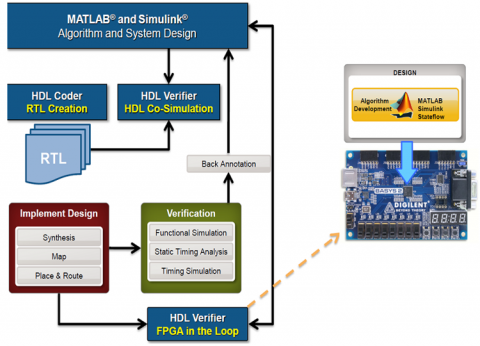
Figure 5 [23] depicts the whole implantation process, including all phases employed in this study, beginning with the use of both Simulink and MATLAB to simulate and analyse the sugested filter design for noise decrease and spike detection. The Verilog HDL (hardware description language) (HDL) coding is then created after the overall system elements have been verified. The (Modelsim De 6.5e) Software and the Synthesis (Integrated Software Environment) (ISE) Suite 14.2 software are used to simulate, validate, and synthesise the LMS model of the adaptive filter on the Embedded system.
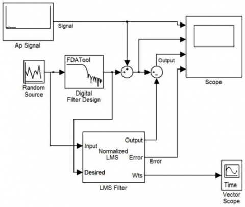
Simulation in MATLAB software was used to assess and test the simulation, as illustrated in Figure 6. The AP signal was combined with a white Gaussian background noise source and filtered using the low-pass FIR. Figure 6 shows the LMS filtering method fed by the Gaussian voltage level and the required signal coupled towards the output data of the LP FIR. The output signal of the LSM adaptive filter removed from a noisy AP signal. The Time Scope is introduced to the system to monitor signal changes and errors during simulation. In addition, the Vector Scope is linked to the filter weights port to display the filter coefficients value.
Figure 5. Design flowchart procedure
Figure 6. Simulink-based LMS adaptive filter model
In Figure 7, time scope window indicates that the error is decreasing and that the output signal is nearly identical to the original neuron pulse input signal.
In Figure 8, vector scope window depicts the actions of LSM model of the adaptive filter coefficients in Simulation result following simulation running time. Figure 8 depicts the filter weights being updated and reaching their steady-state magnitude.
Figure 7. System behaviour in terms of signals
Figure 8. Coefficients for LSM adaptive filters
Table 1. Device usage analysis
|
Design Techniques |
Number of Logic Utilisation |
||||||
|
Slices |
Slice Flip Flops |
4 input LUTs |
bonded IOBs |
Mult18X 18SIOs |
GCLKs |
||
|
Conventional IIR construction |
Used |
301 |
122 |
528 |
23 |
12 |
1 |
|
Utilization |
3% |
0% |
3% |
9% |
42% |
4% |
|
|
Conventional FIR construction |
Used |
369 |
158 |
630 |
35 |
12 |
1 |
|
Utilization |
4% |
0% |
3% |
14% |
42% |
4% |
|
|
LMS adaptive filter construction |
Used |
220 |
100 |
400 |
18 |
8 |
1 |
|
Utilization |
2 % |
0% |
2% |
7% |
28% |
4% |
|
|
|
Available |
8677 |
17344 |
17344 |
250 |
28 |
24 |
Table 2. The power consumption and gate number
|
Power consumption and device usage |
Typical FIR architecture |
Typical IIR architecture |
Typical LMS adaptive filter architecture |
|
No. of logic gates required |
1479,620 |
1,263,513 |
1057,172 |
|
Consumed current |
30 mA |
27 mA |
22 mA |
|
Consumed power (measured) |
30.7 mW |
26.5 mW |
23.6 mW |
|
Consumed power (estimated) |
30.55 mW |
26.36 mW |
23.33 mW |
Figure 9. LMS adaptive filter synthesis process
The Verilog HDL is used to synthesise the suggested filter design using a Xilinx (Spartan 3E-100 xc3s100e) and laptop, as shown in Figure 9. As an ideal length size, the filter input data is digitalized into 16 bits. More optimization is used to reduce electronics size and power usage even further by reducing the amount of multiplications, subtractions and necessary for implementation. The filter is optimised using a parallel processing arrangement in this method.
The greater data sampling frequency is achieved with six clock pulses when the system's clock speed is increased. The hardware design utilisation, which comprises the number of slices, Flip Flops, 4 input LUTs, bonded IOBs, Mult18X18SIOs, and GCLKs, accounts for approximately 25% of the total hardware FPGA size. As a result of adopting a high frequency, the design efficiency is greatly improved. Furthermore, this enhancement improves (VSR) and detection performance in the continuous recording situation.
Table 1 compares the current LMS adaptive filter to another digital filter design, demonstrating that the design occupies around 25% of the hardware space for the xc3s100e Xilinx processor. Furthermore, the device utilisation summary shows that the present design only uses 100 (Flip Flops) slices and 8 (multiplexers) wheel, which is present the most significant improvement can we obtained in this design, whereas the standard IIR and FIR techniques require (122) Flip Flops slices and 12 demux and 158 (Flip Flops) slices and 12 multiplexers, respectively. As a result, the suggested filter architecture offers a significant reduction in hardware size when compared to the classic digital filters techniques (direct IIR and FIR).
The suggested filter mechanism demonstrates a significant reduction in power consumption of roughly 10% and 25% when compared to the IIR and FIR structures, as shown in Table 2. Consequently, this enhancement renders the system more compatible with devices in medical applications, particularly brain recording applications, where power consumption is critical for design manufacture. Furthermore, the noise elimination performance of all streams data recordings enhanced by 23% when compared to other types of filters.
Table 3. Error in suggested LMS adaptive filter and Traditional technique
|
Filter Parameter |
Type of Technique |
Matched Velocity (m/s) |
||||
|
10 |
30 |
50 |
70 |
90 |
||
|
Matched Velocity Band |
Traditional Technique |
1.75 |
16 |
23 |
46 |
45 |
|
Our Technique |
2.7 |
8.9 |
8.3 |
23.9 |
41.6 |
|
|
Centre Velocity(m/s) |
Traditional Technique |
8.87 |
35 |
54.5 |
105 |
107.5 |
|
Our Technique |
10.28 |
32.15 |
51.85 |
70.75 |
93 |
|
|
|Error (m/s)| |
Traditional Technique |
1.13 |
5 |
4.5 |
35 |
17.5 |
|
Our Technique |
0.28 |
2.15 |
1.85 |
0.75 |
3 |
|
As demonstrated in Table 3, the noise reduction improves the precise detection of spikes recordings. This filter's categorization and discrimination are theoretically improved, which implies greater detection, a better accurate ratio, and a lesser missing rate than previous approaches. As a result, this is a conceivable addition to the system that may result in more precise of AP recording, and advanced application for operating prosthetics.
This study proposes an optimal LMS adaptive filter architecture for advanced spike identification utilising VSR in clinical ENG signal recording. The current filter works successfully in a real-time spike recording setting, with improved accuracy performance in a medical application. To evaluate and construct the filter model in both MATLAB and Simulink, a normalise filter approach is employed. The filter configuration is employed a Verilog HDL synthesis on an Embedded system (xc3s100e Xilinx chip). Furthermore, a high-speed sampling data rating is achieved by increasing the system's clock cycle frequency. The arithmetic required for filter setup is minimised, as is the silicon and power necessary to run the system in continuous neural recording without sacrificing accuracy. Approximate 25% in hardware size saving and 10% in power-consuming achieve using ultimate optimum design compare with IIR and FIR filter design. Moreover, the SNR is improved significantly by about 23% for the system.
An innovative spike detection algorithm and hardware implementation designed for online recording multi-channels systems have been presented in this study. The algorithm's key characteristics are as follows: It has a mean-subtraction filter built in that can reduce phase misalignment while eliminating noise. A cutting-edge pre-processor that has the least stated computational complexity of any pre-processor for improving SNR. a brand-new, reliable thresholding scheme that can lessen the impact of surges. This research presents an efficient LMS adaptive filter design for enhanced spike recognition in healthcare ENG signal recording using VSR. In a medical application, the present filter works satisfactorily in a online spike recording situation, with increased accuracy performance. A normalise filter strategy is used to analyse and generate the filter model both in MATLAB and Simulink. On an embedded system, the filter design is implemented using Verilog HDL synthesis (Xilinx chip (xc3s100e)). Furthermore, boosting the system's clock frequency rate results in a high-speed sampling data rate. The mathematics required for filter configuration is reduced, as is the silicon and power required to run the device in continous neural recording mode without compromising accuracy.
The number of single units that can be detected using this approach by spike sorting algorithms is constrained. A ten neurons maximum can be accurately identified at most. This restriction has significant effects on synapses that are sparse. The identification of sparse neurons requires additional algorithmic development.
[1] Agnew, W.F., McCreery, D.B., Yuen, T.G., Bullara, L. A. (1989). Histologic and physiologic evaluation of electrically stimulated peripheral nerve: Considerations for the selection of parameters. Annals of Biomedical Engineering, 17(1): 39-60. https://doi.org/10.1007/BF02364272
[2] Nikolić, Z.M., Popović, D.B., Stein, R.B., Kenwell, Z. (1994). Instrumentation for ENG and EMG recordings in FES systems. IEEE Transactions on Biomedical Engineering, 41(7): 703-6. https://doi.org/10.1109/10.301739
[3] Chapin, J.K., Moxon, K.A. (2001). Neural prostheses for restoration of sensory and motor function. Neuroscience. https://doi.org/10.1201/9781420039054
[4] Hoffer, W.Z., Marks, J.A., Rymer, W.B. (1974). Nerve Fiber Activity During Normal Movements.
[5] Stein, R.B., Charles, D., Davis, L., Jhamandas, J., Mannard, A., Nichols, R.T. (1975). Principles underlying new methods for chronic neural recording. The Canadian Journal of Neurological Sciences. Le Journal Canadien des Sciences Neurologiques, 2(3): 235-244. https://doi.org/10.1017/s0317167100020333
[6] Erlanger, J., Gasser, H. (1937). The comparative physiological characteristics of nerve fibres. In Electrical Signs of Nervous Activity. Philadelphia, PA: Univ. Pennsylvania Press: 34-78.
[7] Hoffer, J.A. (1990). Techniques to Study Spinal Cord Peripheral Nerve and Muscle Activity in Freely Moving Animals. https://doi.org/10.1385/0-89603-185-3:65
[8] Prasanna, Kumar, A.M, Vijaya, S.M. (2020). Noise cancellation employing adaptive digital filters for mobile applications. Indonesian Journal of Electrical Engineering and Informatics (IJEEI), 8(1): 112-122. https://doi.org/10.52549/ijeei.v8i1.1155
[9] Raspopovic, S., Carpaneto, J., Udina, E., Navarro, X., Micera, S. (2010). On the identification of sensory information from mixed nerves by using single channel cuff electrodes. Journal of Neuroengineering and Rehabilitation, 7(1): 17. https://doi.org/10.1186/1743-0003-7-17
[10] Carpenter, R. (1984). Neurophysiology. London: Edward Arnold. https://books.google.iq/books/about/Neurophysiology.html?id=d-1qAAAAMAAJ&redir_esc=y.
[11] Ünsalan, C., Yücel, M.E., Gürhan, H.D. (2018). Digital Signal Processing Using Arm Cortex-M Based Microcontrollers: Theory and Practice. ARM Education Media. https://www.arm.com/resources/education/books/dsptextbook.
[12] Deng, G., Chen, J., Zhang, J., Chang, C. (2019). Area- and power-efficient nearly-linear phase response iir filter by iterative convex optimization. IEEE Access, 7(1): 22952-2965. https://doi.org/10.1109/ACCESS.2019.2899107
[13] Lai, X., Lin, Z. (2016). Iterative reweighted minimax phase error designs of IIR digital filters with nearly linear phases. IEEE Transactions on Acoustics, Speech, and Signal Processing, 64(9): 2416-2428. https://doi.org/10.1109/TSP.2016.2521610
[14] Li, J., Deng, G., Wei, W., Wang, H., Ming, Z. (2017). Design of a real-time ecg filter for portable mobile medical systems. IEEE Access, 5(1): 696-704. https://doi.org/10.1109/ACCESS.2016.2612222
[15] Chen Y., Zhang X., Lian Y., Manohar, R. and Tsividis, Y. (2018). A continuous-time digital iir filter with signal-derived timing and fully agile power consumption. IEEE Journal of Solid-State Circuits, 53(2): 418-430. https://doi.org/10.1109/JSSC.2017.2769339
[16] Al-Shueli, A, Clarke, C.T., Taylor, J.T. (2012). Simulated nerve signal generation for multi-electrode cuff system testing. International Conference on Biomedical Engineering and Biotechnology, 892-896. https://doi.org/10.1109/iCBEB.2012.354
[17] Clarke, T., Xu, X., Rieger, R., Taylor, J., Donaldson, N. (2008). An implanted system for multi-site nerve cuff-based ENG recording using velocity selectivity. Analog Integrated Circuits and Signal Processing, 58(2): 91-104. https://doi.org/10.1007/s10470-008-9233-2
[18] Al-Shueli, A.I., Clarke, C.T., Donaldson, N., Taylor, J.T. (2014). Improved signal processing methods for velocity selective neural recording using multi-electrode cuffs. Biomedical Circuits and Systems, IEEE Transactions, 8(3): 401-410. https://doi.org/10.1109/TBCAS.2013.2277561
[19] Al-Shueli, A.I. (2013). Signal Processing for Advanced Neural Recording Systems. PhD Thesis, University of Bath, Bath, UK. https://researchportal.bath.ac.uk/en/studentTheses/signal-processing-for-advanced-neural-recording-systems.
[20] Taylor, J., Donaldson, N., Winter, J. (2004). Multiple-electrode nerve cuffs for low-velocity and velocity-selective neural recording. Medical & Biological Engineering & Computing, 42(5): 634-643. https://doi.org/10.1007/BF02347545
[21] Kadam, V.S., Gaikwad, A.B. (2015). Design of fpga based adaptive filter based on lms algorithm for echo cancellation. International Journal of Innovations in Engineering Research and Technology, 2015: 1-8.
[22] Sireesha, N., Chithra, K., Sudhaka, T. (2013). Adaptive filtering based on least mean square algorithm. Ocean Electronics (SYMPOL 2013), Conference Proceedings: 42-48. https://doi.org/10.1109/SYMPOL.2013.6701910
[23] Kumar, P. (2012). Generating, Optimising and Verifying HDL Code with MATLAB and Simulink. The MathWorks, Inc.