Abdelouaheb Boukhalfa* | Khatir Khettab | Najib Essounbouli
© 2021 IIETA. This article is published by IIETA and is licensed under the CC BY 4.0 license (http://creativecommons.org/licenses/by/4.0/).
OPEN ACCESS
A Novel hybrid backstepping interval type-2fuzzy adaptive control (HBT2AC) for uncertain discrete-time nonlinear systems is presented in this paper. The systems are assumed to be defined with the aid of discrete equations with nonlinear uncertainties which are considered as modeling errors and external unknown disturbances, and that the observed states are considered disturbed. The adaptive fuzzy type-2 controller is designed, where the fuzzy inference approach based on extended single-input rule modules (SIRMs) approximate the modeling errors, non-measurable states and adjustable parameters are estimated using derived weighted simplified least squares estimators (WSLS). We can prove that the states are bounded and the estimation errors stand in the neighborhood of zero. The efficiency of the approach is proved by simulation for which the root mean squares criteria are used which improves control performance.
interval type 2 fuzzy control, backstepping adaptive control, discrete-time nonlinear system, universal approximator, weighted least squares estimators
The last decades, backstepping technique concerned with strict feedback non-linear systems has been the most important research topic, and it goes a long way towards improving their overall robustness and stabilization. Based on the Lyapunov analysis, the design of feedback control is performed with the choice of an appropriate function in each virtual control input. Dealing with parametric uncertainties and mismatched perturbations of nonlinear systems, the adaptive backstepping control (ABC) has been shown to be an effective approach in order to guarantee asymptotic stability and much contributes to enhance the robustness [1-4].
Adaptive backstepping control (ABC) is one of the popular design methods for a large class of uncertain nonlinear systems, but the problem of “explosion of terms” due to the repeated differentiations of the design of the virtual controller causes relatively limited applications of the ABC. In this context, the authors [5] used the tuning function technique to alleviate this drawback. However, in practical problems, it is almost difficult to determine the upper limits of the most nonlinear uncertainties. Similarly, in the semi-strict feedback nonlinear system, the dynamic surface control procedure has been also used with much less complicated terms. However, the proposed techniques suffer from the measurement uncertainties whose are often nonlinear and immeasurable, and they are limited to SISO nonlinear systems [5-7].
In realistic applications, most systems are complicated and non-linear, which their characteristics can change with time. Due to the nonlinearity, it is difficult to formulate an accurate mathematical model. Therefore, to improve the behavior of adaptive controllers through identifying the unknown nonlinear functions, intelligent approaches such as, artificial neural networks and fuzzy logic [8-11] have been addressed.
Adaptive fuzzy control is mainly categorized into two classes, direct adaptive fuzzy control that its parameters are regulated via the adaptation mechanism [10], while indirect adaptive fuzzy control that its parameters are regulated via the estimated plant based on fuzzy system [11]. In addition, based on the (T-S) models for approximating uncertain nonlinear system in the fuzzy IF-THEN rules, the design of an adaptive fuzzy feedback controller for uncertain nonlinear systems has been reported [1]. However, the designed controller had been developed without considering its unobtainable states and noisy output measurements. Under the aforementioned operating restriction, a nonlinear state observer should be proposed to estimate the immeasurable system states for generating the control signal [12]. Based on the combining of FLC with another control technique, various works were carried out to further demonstrate the enhancement to the control performance including non-linear parametric uncertainties and external disturbances [8, 9, 13].
However, the designed controller had been developed without considering its unobtainable states and noisy output measurements. Under the aforementioned operating restriction, a nonlinear state observer should be proposed to estimate the immeasurable system states for generating the control signal [12]. Then, by using a large number of IF-THEN rules to satisfy the approximation accuracy requirement; a heavy computational burden is inevitably caused, so that the system performance is deteriorated. Therefore, to avoid the so-called “curse of dimensionality”, the single input rule modules have been constructed in various applications. In addition, the SIRMs model which has a simple structure can relatively reduce the number of IF-THEN inference rules and the adjusted parameters [12]. Consequently, to further improve the traditional SIRMs model because of its performance is still limited to deal with high levels of nonlinear uncertainties, an interval type-2 fuzzy logic system (IT2FLS) has been incorporated to replace the ordinary type-1 fuzzy sets [14]. A novel hybrid interval type-2 fuzzy adaptive backstepping control is developed for a class of discrete-time systems with non-linear uncertainties.
To the best of the authors’ knowledge, most research works have only involved uncertain continuous systems without considering the almost unobtainable states. With the aforementioned motivations, by designing state-observers and using the universal approximators [15].
The work is organized as follows. In section 2, we present a nonlinear system described by discrete-time equations with nonlinear uncertainties for which the mathematical models are unknown. A description of the adaptive backstepping control is given in section 3. Section 4 presents the Interval type-2 fuzzy backstepping design. Finally, the application of the proposed method and the simulation results and conclusion are presented in Section 5 and 6.
Let's consider a class of discrete-time uncertain nonlinear systems with modeling errors and unknown external disturbances. we can express the discrete-time uncertain nonlinear systems as:
$x_{i}(k+1)=c_{i} x_{i+1}(k)+\varphi_{i}\left(\overline{\mathbf{x}}_{i}, k\right)$ for $1 \leq i\leq n-1$
$x_{n}(k+1)=c_{n} u(k)+\varphi_{n}(\mathbf{x}, k)$ (1)
the state vector is $\mathbf{x}(k)=\left[x_{1}(k), x_{2}(k), \cdots, x_{n}(k)\right]^{T} \in \mathbb{R}^{n}$ in the Eq. (1), where the sub-state vector is given by $\overline{\mathbf{x}}_{i}(k)=\left[x_{1}(k), x_{2}(k), \cdots, x_{i}(k)\right]^{T} \in \mathbb{R}^{i}(1 \leq i \leq n-1)$ with initial conditions $\mathbf{x}(0)=\mathbf{x}_{0}$ et is the control $\overline{\mathbf{x}}_{i}(0)=\overline{\mathbf{x}}_{i 0}(1 \leq i \leq n-1), u(k) \in \mathbb{R}$ signal, and the nonlinear uncertainty $\varphi_{i}\left(\overline{\mathbf{x}}_{i}, k\right) \in \mathbb{R}, i=1,2, \ldots, n$, which is a combination of the modeling error $m_{i}\left(\overline{\mathbf{x}}_{i}\right) \in \mathbb{R}$ and the unknown external disturbance $d_{i}(k) \in \mathbb{R}$ which is given by:
$\begin{aligned}\left|\varphi_{i}\left(\overline{\mathbf{x}}_{i}, k\right)\right|=\mid m_{i} &\left(\overline{\mathbf{x}}_{i}\right)+d_{i}(k) \mid \leq\left|m_{i}\left(\overline{\mathbf{x}}_{i}\right)\right|+\left|d_{i}(k)\right|, i \\ &=1,2, \ldots, n \leq \operatorname{mos}_{\text {imax }} \| \overline{\mathbf{x}}_{i} \|+d_{\text {imax }} \end{aligned}$ (2)
where, $m_{\text {imax }}$ and $d_{\text {imax }}, i=1,2, \ldots, n$ are positive constants. The coefficient $c_{i}\left(c_{i} \neq 0\right), i=1,2, \ldots, n$ is supposed to be known constants.
A measurement noises affect the observed states as follows:
$y_{i}(k)=x_{i}(k)+v_{i}(k), i=1,2, \ldots, n$ (3)
where, $y_{i}(k) \in R$ is the measure, and $v_{i}(k) \in R$ is the measurement noise.
3.1 Interval type-2 fuzzy adaptive control
To solve the problem of $\varphi_{1}\left(\mathrm{x}_{1}, k\right)$ and $\varphi_{2}\left(\mathrm{x}_{1}, \mathrm{x}_{2}, k\right)$, we approximate them by a two-interval type-2 fuzzy adaptive systems. A fuzzy system that uses fuzzy type 2 sets and inference is a fuzzy type 2 system [10-16]. Type-1 fuzzy set has a crisp membership degree, while type-2 fuzzy set (T2FS) has a fuzzy membership degree. So, type-2 fuzzy systems are "fuzzy-fuzzy" sets that allow better management of uncertainties. One way to represent fuzzy membership of fuzzy sets is using the uncertainty footprint (FOU), which is a 2-D mapping, with uncertainties on the left side of the membership function and also on the right side of the membership function.
Operations of a type-2 fuzzy sets are the same as the operations of a type-1 fuzzy sets, but a type-2 fuzzy system is an interval fuzzy system where the fuzzy operations are performed as two type-1 membership functions, lower membership function (LMF) and upper membership function (UMF) which produce a firing strength [17]. The process of mapping a fuzzy logic control action to a non-fuzzy control action (crisp) is called defuzzification.
A type-2 fuzzy set consists of a two membership functions: primary and secondary. The membership function is a function and not a simple value for each value of the primary variable. Since FOU is not a single point but an interval, the type-2 fuzzy controller can also be referred to as the interval type-2 fuzzy controller. It gives a three-dimensional effect when taking their FOU on a range or an interval. An interval type-2 fuzzy logic-controlled system, has the following architecture: fuzzifier, rule base, fuzzy inference engine, type-reducer and defuzzifier. Type-2 fuzzy systems have been used for modeling and controlling nonlinear systems due to their inherent abilities to approximate nonlinear functions to prescribed accuracies. Based on the universal approximation theorem [15], unknown functions $\varphi_{1}\left(\mathrm{x}_{1}, k\right)$ and $\varphi_{2}\left(\mathrm{x}_{1}, \mathrm{x}_{2}, k\right)$ can be approximated by:
$\hat{\varphi}_{1}\left(\hat{\mathrm{x}}_{1}, k \backslash \theta_{1}\right)=\theta_{1}^{T} \xi_{1}\left(\hat{\mathrm{x}}_{1}\right)$
$\hat{\varphi}_{1}\left(\hat{\mathrm{x}}_{1}, \hat{\mathrm{x}}_{2}, k \backslash \theta_{2}\right)=\theta_{2}^{T} \xi_{2}\left(\hat{\mathrm{x}}_{1}, \hat{\mathrm{x}}_{2}\right)$
where: $\theta_{1}=\left[\theta_{11}, \theta_{12}, \theta_{13}, \theta_{d 1}\right]^{\mathrm{T}}$ and $\theta_{2}=\left[\theta_{211}, \theta_{212}, \theta_{213}, \theta_{222}, \theta_{223}, \theta_{d 2}\right]^{\mathrm{T}}$ are respectively, sets of adjustable parameter vector, $\xi_{1}\left(\hat{x}_{1}\right)=\left[\xi_{11}\left(\hat{x}_{1}\right), \xi_{12}\left(\hat{x}_{1}\right), \xi_{13}\left(\hat{x}_{1}\right), 1\right]^{T}$ and $\xi_{2}\left(\hat{x}_{1}, \hat{x}_{2}\right)=\left[\xi_{211}\left(\hat{x}_{1}\right), \xi_{212}\left(\hat{x}_{1}\right), \xi_{213}\left(\hat{x}_{1}\right), \xi_{221}\left(\hat{x}_{1}\right), \xi_{222}\left(\hat{x}_{1}\right), \right.$$\left. \xi_{223}\left(\hat{x}_{1}\right), 1\right]^{\mathrm{T}}$ are the vector of fuzzy basis functions (FBF), such that:
$\theta_{1}^{T} \xi_{1}\left(\hat{\mathrm{x}}_{1}\right)=\frac{1}{2}\left[\xi_{1 \mathrm{r}}^{\mathrm{T}} \xi_{1 l}^{\mathrm{T}}\right]\left[\theta_{1 \mathrm{r}}^{\mathrm{T}} \theta_{1 l}^{\mathrm{T}}\right]$
$\theta_{2}^{T} \xi_{2}\left(\hat{\mathrm{x}}_{1}, \hat{\mathrm{x}}_{2}\right)=\frac{1}{2}\left[\xi_{2 \mathrm{r}}^{\mathrm{T}} \xi_{2 l}^{\mathrm{T}}\right]\left[\theta_{2 \mathrm{r}}^{\mathrm{T}} \theta_{2 l}^{\mathrm{T}}\right]$
where: $\xi_{l}=\left[\xi_{l}^{1}, \xi_{l}^{2}, \ldots, \xi_{l}^{\mathrm{m}}\right]^{\mathrm{T}}, \quad \xi_{r}=\left[\xi_{r}^{1}, \xi_{r}^{2}, \ldots, \xi_{r}^{\mathrm{m}}\right]^{\mathrm{T}}$, $\theta_{r}=\left[\theta_{1 r}, \theta_{2 r}, \ldots, \theta_{m r}\right]$ and $\theta_{l}=\left[\theta_{1 l}, \theta_{2 l}, \ldots, \theta_{m l}\right]$.
This yields the minimum approximation error:
$\varepsilon_{1}(k)=\varphi_{1}\left(\mathrm{x}_{1}, k\right)-\theta_{1}^{\mathrm{T}}(k) \xi_{1}(k)\left(\hat{\mathrm{x}}_{1}\right)$
$\varepsilon_{2}(k)=\varphi_{2}\left(\mathrm{x}_{1}, \mathrm{x}_{2}, k\right)-\theta_{2}^{\mathrm{T}}(k) \xi_{2}(k)\left(\hat{\mathrm{x}}_{1}, \hat{\mathrm{x}}_{2}\right)$
3.2 Fuzzy inference approach
Let $x_{i}, i=1,2, \ldots, n$ and $y$ are, respectively, the input and the output, the IF-THEN fuzzy rules are given by:
$\begin{array}{ll}R^{j}: & I F x_{1} \text { is } A_{1}^{j} \ldots x_{i} \text { is } A_{i}^{j} \ldots x_{n} \text { is } A_{n}^{j} \text { THENy is B }^{j} \\ & j=1,2, \ldots, p\end{array}$ (4)
where, $R^{j}$ is the $j^{t h}$ fuzzy rule IF-THEN, and $A_{i}^{j}$ and $B_{i}^{j}$ are the fuzzy sets with $\mu_{A i}^{j}\left(x_{i}\right)$ and $\mu_{B}^{j}\left(x_{i}\right)$ as membership functions respectively. Fuzzy inference engine performs a mapping of fuzzy sets in $\mathbf{R}^{n}$ into the fuzzy set in Ron the basis of the IF-THEN fuzzy rules given in Eq. (4). However, since the number of IF-THEN fuzzy rules must be large to enhance the precision of the approximation, consequently, the adjustable parameters number will increase exponentially as the number of IF-THEN fuzzy rules increases. Then, the control performance is degraded due to the heavy computational load and increases the operating costs. As a result, a fuzzy inference approach based on the extended SIRMs to reduce the computational load is used [18]. Denoting $x_{i}, i=1,2, \ldots, n$ and $y_{i}, i=1,2, \ldots, n$ are respectively the input and the output, the IF-THEN fuzzy rules based on extended single input rule modules are described as follows:
$R_{1}^{j}:$ IF $x_{1}$ is $A_{1}^{j}$ THEN $y_{1}$ is $B_{1}^{j}, j=1,2, \ldots, r$
$\vdots$
$R_{i}^{j}:$ IF $x_{i}$ is $A_{i}^{j}$ THEN $y_{i}$ isB $_{i}^{j}, j=1,2, \ldots, r$
$\vdots$
$R_{n}^{j}:$ IF $x_{n}$ is $A_{n}^{j}$ THEN $y_{n}$ is $B_{n}^{j}, j=1,2, \ldots, r$ (5)
where, $A_{i}^{j}$ and $B_{i}^{j}$ are the fuzzy sets whose membership functions are respectively $\mu_{A i}^{j}\left(x_{i}\right)$, and $\mu_{B i}^{j}\left(x_{i}\right)$. By means of singleton fuzzification strategy, defuzzification by center of gravity and product inference, the fuzzy system output is given as follows:
$y=\sum_{i=1}^{n} \theta_{i}^{T} \xi_{i}\left(\mathbf{x}_{i}\right)=\theta^{T} \xi(\mathbf{x})$ (6)
where,
$\theta=\left[\theta_{1}^{T}, \ldots, \theta_{i}^{T}, \ldots, \theta_{n}^{T}\right]^{T} \in \mathbf{R}^{s}$
$\xi(\mathbf{x})=\left[\xi_{1}^{T}\left(x_{1}\right), \ldots, \xi_{i}^{T}\left(x_{i}\right), \ldots, \xi_{n}^{T}\left(x_{n}\right)\right]^{T} \in \mathbf{R}^{s}$
are, sets of the adjustable parameters vector of $\theta_{i}$ and the fuzzy basis function vector $\xi_{i}\left(x_{i}\right)$ respectively, where:
$\theta_{i}=\left[\theta_{i 1}, \ldots, \theta_{i j}, \ldots, \theta_{i r}\right]^{T} \in \mathbf{R}^{r}$
$\xi_{i}\left(x_{i}\right)=\left[\xi_{i 1}\left(x_{i}\right), \ldots, \xi_{i j}\left(x_{i}\right), \ldots, \xi_{i r}\left(x_{i}\right)\right]^{T} \in \mathbf{R}^{r}$
with the $j^{t h}$ column $\xi_{i j}\left(x_{i}\right)$ of $\xi_{i}\left(x_{i}\right)$ given as follows:
$\xi_{i j}\left(x_{i}\right)=\frac{\mu_{A i}^{j}\left(x_{i}\right)}{\sum_{j=1}^{r} \mu_{A i}^{j}\left(x_{i}\right)}, j=1,2, \ldots, r$ (7)
A fuzzy system is given by the Eq. (6) which approximate $y$ as $\theta^{T} \xi(x)$ on a compact set U based on the universal approximation theorem to an arbitrary precision [15].
3.3 Fuzzy inference approach based on extended single-input rule modules
Based on the extended single input rule modules, using the IF-THEN fuzzy rules, the modeling error $m_{i}\left(\overline{\mathbf{x}}_{i}\right)$ is estimated as $\widehat{\mathbf{m}}_{i}\left(\overline{\mathbf{x}}_{i} \mid \boldsymbol{\theta}_{\mathbf{i}}\right)$, where $\overline{\mathbf{x}}_{i}(k)$ is the estimate of $\overline{\mathbf{x}}_{i}(k)$. Let $\hat{x}_{l}(k), l=1,2, \ldots, i$ for the input and for the output $\widehat{m}_{i}\left(\overline{\mathbf{x}}_{i} \mid \boldsymbol{\theta}_{\mathbf{i}}\right)$, The fuzzy rules IF-THEN based on extended single input rule modules are given as follows:
$R_{1}^{j}: I F \widehat{x}_{1}(k) \text { is } A_{1}^{j} T H E N \hat{m}_{i}\left(\hat{\mathbf{x}}_{i} \mid \theta_{i 1}\right) \text { is } B_{1}^{j}, j=1,2, \ldots, r$
$\quad \vdots$
$R_{l}^{j}: I F \widehat{X}_{l}(k) \text { is } A_{l}^{j} T H E N \hat{m}_{i}\left(\hat{\mathbf{x}}_{i} \mid \theta_{i l}\right) \text { is } B_{l}^{j}, j=1,2, \ldots, r$
$\quad \vdots$
$R_{i}^{j}: I F \hat{X}_{i}(k) \text { is } A_{i}^{j} T H E N \hat{m}_{i}\left(\hat{\mathbf{x}}_{i} \mid \theta_{i i}\right) \text { is } B_{i}^{j}, j=1,2, \ldots, r$ (8)
where, $A_{l}^{j}$ and $B_{l}^{j}$ are a fuzzy sets with membership functions are, $\mu_{A l}^{j}\left[\hat{x}_{l}(k)\right]$ and $\mu_{B l}^{j}\left[{\hat{m}_{i}\left(\bar{x}_{i} \mid \theta_{i}\right)}\right]$, respectively. By means of the singleton fuzzification strategy, center of gravity defuzzification, and product inference, the output is given by:
$\widehat{m}_{i}\left(\hat{\overline{\mathbf{x}}}_{i} \mid \theta_{i}\right)=\theta_{i}^{T} \xi_{i}\left(\hat{\overline{\mathbf{x}}}_{i}\right)$ (9)
where,
$\theta_{i}=\left[\theta_{i 1}^{T}, \ldots, \theta_{i l}^{T}, \ldots, \theta_{i i}^{T}\right]^{T} \in \mathbf{R}^{(i \times r)}$
$\xi_{i}\left(\hat{\bar{x}}_{i}\right)=\left[\xi_{i 1}^{T}\left(\hat{x}_{1}\right), \ldots, \xi_{i l}^{T}\left(\hat{x}_{l}\right), \ldots, \xi_{i i}^{T}\left(\hat{x}_{i}\right)\right]^{T} \in \mathbf{R}^{(i \times r)}$
are the sets of adjustable parameter vectors and fuzzy basis function vectors, respectively, with $\xi_{i l j}\left(\hat{x}_{l}\right)$ of $\xi_{i l}\left(\hat{x}_{l}\right)$ given as [19]:
$\xi_{i l j}\left(\hat{x}_{l}\right)=\frac{\mu_{A l}^{j}\left(\hat{x}_{l}\right)}{\sum_{j=1}^{r} \mu_{A l}^{j}\left(\hat{x}_{l}\right)}, j=1,2, \ldots, r$ (10)
Because the external unknown disturbance $d_{i}(k)$ is supposed as a time function, we can include it in $\theta_{i}$ and $\xi_{i}\left(\hat{\bar{x}}_{i}\right)$, respectively, in the Eq. (9), then:
$\theta_{i}=\left[\theta_{i 1}^{T}, \ldots, \theta_{i l}^{T}, \ldots, \theta_{i i}^{T}, \theta_{i d}\right]^{T} \in \mathbf{R}^{(i \times r+1)}$
$\xi_{i}\left(\hat{\bar{x}}_{i}\right)=\left[\xi_{i 1}^{T}\left(\hat{x}_{1}\right), \ldots, \xi_{i l}^{T}\left(\hat{x}_{l}\right), \ldots, \xi_{i i}^{T}\left(\hat{x}_{i}\right), 1\right]^{T}\in \mathbf{R}^{(i \times r+1)}$
where, $\theta_{i d}$ and 1 denote $d_{i}(k)=\theta_{i d} \times 1$. Then the Eq. (9) is rewritten as:
$\hat{\varphi}_{i}\left(\hat{\overline{\mathbf{x}}}_{i}, k \mid \theta_{i}\right)=\theta_{i}^{T} \xi_{i}\left(\hat{\overline{\mathbf{x}}}_{i}\right)$ (11)
An adaptive fuzzy backstepping controller (AFBC) $u_{a f b}(k)$ is designed, $\varphi_{i}\left(\bar{x}_{i}, k\right)$ is approximated based on $\widehat{\varphi}_{i}\left(\hat{\overline{\mathbf{x}}}, k \mid \theta_{i}^{*}\right)$ using a type-2 fuzzy inference approach which is based on extended single-input rule modules, where $\theta_{i}^{*}$ is the optimal parameter vector defined as follows [14, 20].
where, $\Omega_{i}, U_{i}$ and $V_{i}$ are respectively, suitable compact sets. Since $\theta_{i}^{*}$ is an artificial quantity required for an analytical purpose, it is treated as an unknown vector, but it is designated as the reference of $\theta_{i}$. By defining the universal approximation error $\varepsilon_{i}(k)$ and the vector of estimation error $\tilde{x}_{i}(k)$, respectively, as $\left[\varphi_{i}\left(\bar{x}_{i}, k\right)-\hat{\varphi}_{i}\left(\hat{\bar{x}}_{i}, k \mid \theta_{i}^{*}\right)\right]$ and $\left[x_{i}(k)-\hat{x}_{i}(k)\right]$, the adaptive fuzzy backstepping control (AFBC) is proposed as follows [21, 22]:
$\begin{aligned} \theta_{i}^{*} &=\arg \min _{\theta_{i} \in \Omega_{i}}\left[\sup _{\bar{x}_{i} \in U_{i}, \bar{x}_{i} \in V_{i}}\left|\varphi_{i}\left(\overline{\mathbf{x}}_{i}, k\right)-\hat{\varphi}_{i}\left(\hat{\overline{\mathbf{x}}}_{i}, k \mid \theta_{i}\right)\right|\right], \\ & i=1,2, \ldots, n \end{aligned}$ (12)
4.1 Step 1: (i=1)
Let’s define $e_{1}(k)=x_{1}(k)$ in Eq. (1) for $i=1, x_{2 d}(k)$ is the virtual control given by:
$\hat{x}_{2 d}(k)=\frac{1}{c_{1}}\left[k_{1} \hat{e}_{1}(k)-\hat{\varphi}_{1}\left(\hat{\overline{\mathbf{x}}}_{1}, k \mid \theta_{1}^{*}\right)\right]$ (13)
where, $\hat{e}_{1}(k)$ is the estimate for $e_{1}(k)$, and $\hat{x}_{1 d}(k)=0$. By substituting the Eq. (13) in the Eq. (1) for i=1 becomes:
$e_{1}(k+1)=k_{1} e_{1}(k)+c_{1} e_{2}(k)-k_{1} \tilde{x}_{1}(k)+\varepsilon_{1}(k)$ (14)
4.2 Step i: $(2 \leq i \leq n-1)$
Let’s define $e_{i}(k+1)=x_{i}(k+1)-\hat{x}_{i d}(k+1)$ and substituting it in (1) for $(2 \leq i \leq n-1)$ gives:
$e_{i}(k+1)=c_{i} x_{i+1}(k)+\varphi_{i}\left(\overline{\mathbf{x}}_{i}, k\right)-\hat{x}_{i d}(k+1)$ (15)
Then, the virtual control $\hat{x}_{(i+1) d}(k)$ is
$\hat{x}_{(i+1) d}(k)=\frac{1}{c_{i}}\left[k_{i} \hat{e}_{i}(k)-\hat{\varphi}_{i}\left(\hat{\overline{\mathbf{x}}}_{i}, k \mid \theta_{i}^{*}\right)+\hat{x}_{i d}(k+1)\right]$ (16)
where, $\widehat{e}_{i}(k)$ is the estimate of $e_{i}(k)$ The substitution of the Eq. (16) in (15) provides
$e_{i}(k+1)=k_{i} e_{i}(k)+c_{i} e_{i+1}(k)-k_{i} \tilde{x}_{i}(k)+\varepsilon_{i}(k)$ (17)
4.3 Step n:
Let’s define $e_{n}(k+1)=x_{n}(k+1)-\hat{x}_{n d}(k+1)$, The Eq. (1) for i=n is as follows:
$e_{n}(k+1)=c_{n} u(k)+\varphi_{n}(\mathbf{x}, k)-\hat{x}_{n d}(k+1)$ (18)
Then, the control $u_{a f b}(k)$ is:
$u_{a f b}(k)=\frac{1}{c_{n}}\left[k_{n} \hat{e}_{n}(k)-\hat{\varphi}_{n}\left(\hat{\mathbf{x}}, k \mid \theta_{n}^{*}\right) +\hat{x}_{n d}(k+1)\right]$ (19)
where, $\hat{e}_{n}(k)$ is the estimate of $e_{n}(k)$. The substitution of the Eq. (19) in the Eq. (18) provides:
$e_{n}(k+1)=k_{n} e_{n}(k)-k_{n} \tilde{x}_{n}(k)+\varepsilon_{n}(k)$ (20)
Let’s define the state vector $\mathbf{e}(k)=\left[e_{1}(k), e_{2}(k), \ldots, e_{n}(k)\right]^{T} \in \mathbf{R}^{n}$, the state equation is expressed as follows:
$\mathbf{e}(k+1)=\mathbf{F}_{e} \mathbf{e}(k)-\mathbf{F}_{x} \tilde{\mathbf{x}}(k)+\boldsymbol{\varepsilon}(k)$ (21)
where, $\widetilde{\mathbf{x}}(k) \in \mathbf{R}^{n}$ is the vector of the estimation error, $\varepsilon(k) \in \mathbf{R}^{n}$ is the vector of the universal approximation error, and $\mathbf{F}_{e} \in \mathbf{R}^{n \times n}$ and $\mathbf{F}_{x} \in \mathbf{R}^{n \times n}$ are matrices which are constants, respectively, defined as:
$\tilde{\mathbf{x}}(k)=\left[\tilde{x}_{1}(k), \tilde{x}_{2}(k), \ldots, \tilde{x}_{n}(k)\right]^{T}$
$\varepsilon(k)=\left[\varepsilon_{1}(k), \varepsilon_{2}(k), \ldots, \varepsilon_{n}(k)\right]^{T}$
$\mathbf{F}_{e}=\left[\begin{array}{lllll}k_{1} & c_{1} & 0 & \ldots & 0 \\ 0 & k_{2} & c_{2} & 0 & \vdots \\ \vdots & 0 & \ddots & \ddots & 0 \\ \vdots & \vdots & \ddots & \ddots & c_{n-1} \\ 0 & & & 0 & k_{n}\end{array}\right]$,
$\mathbf{F}_{x}=\left[\begin{array}{lllll}k_{1} & 0 & \ldots & \ldots & 0 \\ 0 & k_{2} & 0 & \ldots & \vdots \\ \vdots & 0 & \ddots & \ddots & \vdots \\ \vdots & \vdots & \ddots & \ddots & 0 \\ 0 & & & 0 & k_{n}\end{array}\right]$
Theorem 1: Subject to the proposed control $u_{a f b}(k), e(k)$ given in Eq. (21) is bounded, if Fe is stable, and the terms in second and third of the second side of the Eq. (21) are bounded. Therefore, to obtain a simplified control $\bar{u}_{a f b}(k)$ an approach is presented as follows. Let’s Consider Eqns. (13) and (16), $\hat{x}_{i d}(k+1)$ and $\hat{x}_{n d}(k+1)$ in the Eqns. (16) and (19) are approximately given as:
$\hat{x}_{i d}(k+1)=\left(1-\lambda_{i}\right) \hat{x}_{i d}(k)+\lambda_{i}\left[k_{i-1} \hat{e}_{i-1}(k)\right.$
$\left.-\hat{\varphi}_{i-1}\left(\hat{\overline{\mathbf{x}}}_{i-1}, k \mid \theta_{i-1}^{*}\right)\right]$ (22)
$\left.\hat{x}_{n d}(k+1)=1-\lambda_{n}\right) \hat{x}_{n d}(k)+\lambda_{n}\left[k_{n-1} \hat{e}_{n-1}(k)\right.$
$\left.-\hat{\varphi}_{n-1}\left(\hat{\overline{\mathbf{x}}}_{n-1}, k \mid \theta_{n-1}^{*}\right)\right]$ (23)
For the Eqns. (22) and (23), $\lambda_{i}<1, i=2,3, \ldots, n$, is a positive constant. If we substitute the Eqns. (22) and (23) in the Eqns. (16) and (19), respectively, it provides:
$\begin{aligned} \hat{x}_{(i+1) d}(k) &=\frac{1}{c_{i}}\left[k_{i} \hat{e}_{i}(k)-\hat{\varphi}_{i}\left(\hat{\overline{\mathbf{x}}}_{i}, k \mid \theta_{i}^{*}\right)+\lambda_{i} k_{i-1} \hat{e}_{i-1}(k)\right.\\ &\left.-\lambda_{i} \hat{\varphi}_{i-1}\left(\hat{\overline{\mathbf{x}}}_{i-1}, k \mid \theta_{i-1}^{*}\right)+\left(1-\lambda_{i}\right) \hat{x}_{i d}(k)\right] \\ &=\frac{1}{c_{i}}\left[k_{i} \hat{x}_{i}(k)+\lambda_{i} k_{i-1} \hat{x}_{i-1}(k)-\hat{\varphi}_{i}\left(\hat{\overline{\mathbf{x}}}_{i}, k \mid \theta_{i}^{*}\right)\right.\\ &-\lambda_{i} \hat{\varphi}_{i-1}\left(\hat{\overline{\mathbf{x}}}_{i-1}, k \mid \theta_{i-1}^{*}\right)-\lambda_{i} k_{i-1} \hat{x}_{(i-1) d}(k) \\ &\left.+\left(1-k_{i}-\lambda_{i}\right) \hat{x}_{i d}(k)\right] \end{aligned}$ (24)
$\begin{aligned} \bar{u}_{a f b}(k)=& \frac{1}{c_{n}}\left[k_{n} \hat{e}_{n}(k)-\hat{\varphi}_{n}\left(\hat{\mathbf{x}}, k \mid \theta_{n}^{*}\right)+\lambda_{n} k_{n-1} \hat{e}_{n-1}(k)\right.\\ &\left.-\lambda_{n} \hat{\varphi}_{n-1}\left(\hat{\overline{\mathbf{x}}}_{n-1}, k \mid \theta_{n-1}^{*}\right)+\left(1-\lambda_{n}\right) \hat{x}_{n d}(k)\right] \\=& \frac{1}{c_{n}}\left[k_{n} \hat{x}_{n}(k)+\lambda_{n} k_{n-1} \hat{x}_{n-1}(k)-\hat{\varphi}_{n}\left(\hat{\mathbf{x}}, k \mid \theta_{n}^{*}\right)\right.\\ &-\lambda_{n} \hat{\varphi}_{n-1}\left(\hat{\overline{\mathbf{x}}}_{n-1}, k \mid \theta_{n-1}^{*}\right)-\lambda_{n} k_{n-1} \hat{x}_{(n-1) d}(k) \\ &\left.+\left(1-k_{n}-\lambda_{n}\right) \hat{x}_{n d}(k)\right] \end{aligned}$ (25)
The repeated execution of the recursive relation (24), for $i=2,3, \ldots, n-1, \hat{x}_{(n-1) d}(k)$ and $\hat{x}_{n d}(k)$ are obtained with the initial condition given by:
$\hat{x}_{1 d}(k)=0, \hat{x}_{2 d}(k)=\frac{1}{c_{1}}\left[k_{1} \hat{x}_{1}(k)-\boldsymbol{\varphi}_{i}\left(\hat{\bar{x}}_{1}, k \mid \theta_{i}^{*}\right)\right]$
By substituting $\hat{x}_{(n-1) d}(k)$ and $\hat{x}_{n d}(k)$ in the Eq. (25), we obtain $\bar{u}_{a f b}(k)$.
4.4 Least squares estimators
The state equation, based on the Eq. (1), is defined as:
$\mathbf{x}(k+1)=\mathbf{F} \mathbf{x}(k)+\widehat{\boldsymbol{\varphi}}\left(\hat{\mathbf{x}}, k \mid \theta^{*}\right)$
$+\mathbf{g} \bar{u}_{a f b}(k)+\boldsymbol{\varepsilon}(k)$ (26)
where, $\mathbf{x}(k) \in \mathbf{R}^{n}, \hat{\varphi}\left(\hat{x}, k \mid \theta^{*}\right) \in \mathbf{R}^{n}, \mathbf{F} \in \mathbf{R}^{n \times n}$, and $\mathbf{g} \in \mathbf{R}^{n}$ are, respectively, defined as:
$\hat{\varphi}\left(\hat{\mathbf{x}}, k \mid \theta^{*}\right)$
$=\left[\hat{\varphi}_{1}\left(\hat{\mathbf{x}}_{1}, k \mid \theta_{1}^{*}\right), \hat{\varphi}_{2}\left(\hat{\mathbf{x}}_{2}, k \mid \theta_{2}^{*}\right), \ldots, \hat{\varphi}_{n}\left(\widehat{\mathbf{x}}, k \mid \theta_{n}^{*}\right)\right]^{T}$
$\mathbf{F}=\left[\begin{array}{lllll}0 & c_{1} & 0 & \cdots & 0 \\ \vdots & 0 & c_{2} & 0 & \vdots \\ \vdots & \vdots & 0 & \ddots & 0 \\ \vdots & \vdots & \vdots & \ddots & c_{n-1} \\ 0 & \cdots & \cdots & \cdots & 0\end{array}\right]$,
$\mathbf{g}=\left[\begin{array}{lllll}0, & 0, & \cdots & 0, & c_{n}\end{array}\right]^{T}$
Using the Eq. (11), the Eq. (26) provides
$\mathbf{x}(k+1)=\mathbf{F x}(k)+\mathbf{F}_{\boldsymbol{\varphi}}(\hat{\mathbf{x}}, k) \theta^{*}$
$+\mathbf{g} \bar{u}_{a f b}(k)+\boldsymbol{\varepsilon}(k)$ (27)
where, $\mathbf{F}_{\boldsymbol{\varphi}}(\widehat{\mathbf{x}}, k) \in \mathbf{R}^{n \times s}$ and $\varepsilon(k)$ are, respectively, expressed as:
$\mathbf{F}_{\varphi^{\mathbf{F}}} (\hat{\mathbf{x}}, k)=\left[\begin{array}{lllll}\xi_{1}\left(\hat{\overline{\mathbf{x}}}_{1}\right) & 0 & \cdots & \cdots & 0 \\ 0 & \xi_{2}\left(\hat{\overline{\mathbf{x}}}_{2}\right) & 0 & \cdots & \vdots \\ \vdots & 0 & \ddots & \ddots & \vdots \\ \vdots & \vdots & \vdots & \ddots & 0 \\ 0 & \cdots & \cdots & 0 & \xi_{n}(\hat{\mathbf{x}})\end{array}\right]$
$\boldsymbol{\varepsilon}(k)=\varphi(\mathbf{x}, k)-\mathbf{F}_{\varphi}(\hat{\mathbf{x}}, k) \theta^{*}$ (28)
By designing the WLSE and SWLSE to involve estimates of non-measurable states and adjustable parameters, a set measurement of noises is used. We can see that under the idea that nonlinearity is negligible, the performance of the least squares estimator in estimating unmeasurable states and uncertainties has been improved, and nonlinearity can usually obtain sufficient information from the measurement equation. However, sometimes there will be such an impression that because the nonlinear high-order terms are not negligible, the estimation error will be greatly reduced or diverged. As a method to enhance the degradation and difference of estimation errors, WLSE [12, 18] is proposed, which is obtained by putting higher weight on newer output information. In the design of WLSE, the extended state equation is given by the following formula:
$\mathbf{x}_{a}(k+1)=\Phi\left(\hat{\mathbf{x}}_{a}, k\right) \mathbf{x}_{a}(k)+\mathbf{g}_{a} \bar{u}_{a f b}(k)+\boldsymbol{\varepsilon}_{a}(k)$ (29)
where, $\mathbf{x}_{a}(k) \in \mathbf{R}^{n+s}$ is the augmented state vector, $\Phi\left(\hat{x}_{a}, k\right) \in \mathbf{R}^{(n+s) \times(n+s)}$ is the transition matrix, and $\mathbf{g}_{a} \in \mathbf{R}^{n+s}$ is the driving matrix, defined as, respectively:
$\begin{aligned} \mathbf{x}_{a}(k)=&\left[\begin{array}{l}\mathbf{x}(k) \\ \theta^{*}\end{array}\right], \Phi\left(\hat{\mathbf{x}}_{a}, k\right)=\left[\begin{array}{ll}\mathbf{F} & \mathbf{F}_{\boldsymbol{\varphi}}(\hat{\mathbf{x}}, k) \\ \mathbf{0} & \mathbf{I}\end{array}\right] \\ & \mathrm{g}_{a}=\left[\begin{array}{l}\mathrm{g} \\ 0\end{array}\right], \varepsilon_{a}(k)=\left[\begin{array}{l}\varepsilon(k) \\ 0\end{array}\right] \end{aligned}$
While the augmented measurement equations come from Eq. (4) given by:
$\mathbf{y}(k)=\mathbf{H}_{a} \mathbf{x}_{a}(k)+\mathbf{v}(k)$ (30)
where, $\mathbf{y}(k) \in \mathbf{R}^{n}, \mathbf{v}(k) \in \mathbf{R}^{n} \quad$ and $\quad \mathbf{H}_{a} \in \mathbf{R}^{n \times(n+s)}$ are, respectively, defined as:
$\mathbf{y}(k)=\left[y_{1}(k), y_{2}(k), \ldots, y_{n}(k)\right]^{T}$
$\mathbf{v}(k)=\left[v_{1}(k), v_{2}(k), \ldots, v_{n}(k)\right]^{T}$
$\mathbf{H}_{a}=[\mathbf{I} \mathbf{0}]$
Assume that the measurement to require the estimate $\widehat{\mathbf{x}}_{a}(k)$ for $\mathbf{x}_{a}(k)$ in the design of the WLSE is given by:
$\begin{aligned} J_{e}=& \sum_{i=1}^{k+1}\left[\mathbf{y}(i)-\mathbf{H}_{a} \mathbf{x}_{a}\right]^{T} \exp \left[-c_{v}(k+1-i)\right] \mathbf{R}_{v}^{-1} \\ & \times\left[\mathbf{y}(i)-\mathbf{H}_{a} \mathbf{x}_{a}(i)\right]+\tilde{\mathbf{x}}_{a}^{T} \mathbf{P}_{a}^{-1}(0) \tilde{\mathbf{x}}_{a}(0) \end{aligned}$ (31)
under the Eq. (29), where $\mathbf{R}_{v} \in \mathbf{R}^{n \times n}$ and $\mathbf{P}_{a}(0) \in \mathbf{R}^{(n+s) \times(n+s)}$ are positive definite matrices which correspond respectively, to the covariance for $\mathbf{v}(i)$ and $\tilde{\mathbf{x}}_{a}(0)$. In measuring, $\mathbf{R}_{v}$ is changed to $\exp \left[c_{v}(k+1-i)\right] \mathbf{R}_{v}$, where $c_{v}$ may be a small positive constant, which means that in the derivation of WLSE, a newer output information is being forced to require $ \hat{\mathbf{x}}_{a}(k)$. Neglect $\varepsilon_{a}(k)$ within the Eq. (29), $ \hat{\mathbf{x}}_{a}(k)$ is derived as follows [12, 18]:
$\hat{\mathbf{x}}_{a}(k+1)=\hat{\mathbf{x}}_{a}(k+1 \mid k)+\mathbf{K}_{a}(k+1) \times[\mathbf{y}(k+1)-\hat{\mathbf{y}}(k+1 \mid k)]$ (32)
$\hat{\mathbf{x}}_{a}(k+1 \mid k)=\boldsymbol{\Phi}\left(\hat{\mathbf{x}}_{a}, k\right) \hat{\mathbf{x}}_{a}(k)+\mathbf{g}_{a} \bar{u}_{f a b}(k)$ (33)
$\hat{\mathbf{y}}(k+1 \mid k)=\mathbf{H}_{a} \hat{\mathbf{x}}_{a}(k+1 \mid k)$ (34)
$\begin{aligned} \mathbf{K}_{a}(k+1) &=\exp \left(c_{v}\right) \mathbf{P}_{a}(k+1 \mid k) \mathbf{H}_{a}^{T} \\ & \times\left[\mathbf{H}_{a} \exp \left(c_{v}\right) \mathbf{P}_{a}(k+1 \mid k) \mathbf{H}_{a}^{T}+\mathbf{R}_{v}\right]^{-1} \end{aligned}$ (35)
$\mathbf{P}_{a}(k+1)=\left[\mathbf{I}-\mathbf{K}_{a}(k+1) \mathbf{H}_{a}\right] \exp \left(c_{v}\right) \mathbf{P}_{a}(k+1 \mid k)$ (36)
$\mathbf{P}_{a}(k+1 \mid k)=\boldsymbol{\Phi}\left(\hat{\mathbf{x}}_{a}, k\right) \mathbf{P}_{a}(k) \boldsymbol{\Phi}^{T}\left(\hat{\mathbf{x}}_{a}, k\right)$ (37)
with the initial conditions given by $\hat{\mathbf{x}}_{a}(0)$ and $\mathbf{P}_{a}(0)$. Based on the WLSE, the vector of the estimation error $\tilde{\mathbf{x}}_{a}(k) \in \mathbf{R}^{n+s}$ defined as $\left[\mathbf{x}_{a}(k)-\hat{\mathbf{x}}_{a}(k)\right]$ is derived. The Eq. (32) is subtracted from the Eq. (29), and the vector of error estimation $\tilde{\mathbf{x}}_{a}(k)$ is given by:
$\begin{aligned} \tilde{\mathbf{x}}_{a}(k+1) &=\boldsymbol{\Phi}_{a}\left(\hat{\mathbf{x}}_{a}, k\right) \tilde{\mathbf{x}}_{a}(k)+\varepsilon_{a}(k)-\mathbf{K}_{a}(k+1) \\ & \times\left[\mathbf{H}_{a} \boldsymbol{\Phi}_{a}\left(\hat{\mathbf{x}}_{a}, k\right) \tilde{\mathbf{x}}_{a}(k)+\mathbf{H}_{a} \varepsilon_{a}(k)+\mathbf{v}(k+1)\right] \\ &=\left[\mathbf{I}-\mathbf{K}_{a}(k+1) \mathbf{H}_{a}\right] \tilde{\mathbf{x}}_{a}(k+1 \mid k) \\ &-\mathbf{K}_{a}(k+1) \mathbf{v}(k+1) \end{aligned}$ (38)
where,
$\tilde{\mathbf{x}}_{a}(k+1 \mid k)=\boldsymbol{\Phi}_{a}\left(\hat{\mathbf{x}}_{a}, k\right) \tilde{\mathbf{x}}_{a}(k)+\varepsilon_{a}(k)$ (39)
Theorem 2- The vector of the estimation error $\tilde{\mathrm{x}}_{\mathrm{a}}(\mathrm{k})$ in (38) and (39) will saty in the neighborhoud of zero, if $\varepsilon_{\mathrm{a}}(\mathrm{k}) \mathrm{x}_{\mathrm{a}}(\mathrm{k})$, and $\widehat{\mathrm{x}}_{\mathrm{a}}(\mathrm{k})$ are bounded.
The SWLSE is calculated by approximating the structure of the WLSE, to reduce the computational burden of the estimate. The estimates $\hat{\mathbf{x}}(k)$ and $\theta_{i}(k)$, for $\mathbf{x}(k)$ and $\theta_{i}^{*}$ are given by:
$\begin{aligned} \hat{\mathbf{x}}(k+1) &=\mathbf{F} \hat{\mathbf{x}}(k)+\mathbf{F}_{\varphi}(\hat{\mathbf{x}}, k) \boldsymbol{\theta}(k)+\mathbf{g} \bar{u}_{f a b}(k) \\ &+\mathbf{K}_{x}(k+1)[\mathbf{y}(k+1)-\hat{\mathbf{y}}(k+1 \mid k)] \end{aligned}$ (40)
$\begin{aligned} \boldsymbol{\theta}_{i}(k+1) &=\boldsymbol{\theta}_{i}(k)+\exp \left(c_{v}\right) \mathbf{P}_{\theta i}(k) \xi_{i}(\overline{\mathbf{x}}, k) \Omega_{i i}^{-1}(k) \\ & \times\left[y_{i}(k+1)-\hat{y}_{i}(k+1 \mid k)\right] \\ & i=1,2, \ldots, n \end{aligned}$ (41)
$\begin{aligned} \mathbf{K}_{x}(k+1) &=\exp \left(c_{v}\right)\left[\mathbf{F} \mathbf{P}_{x}(k) \mathbf{F}^{T}\right.\\ &\left.+\mathbf{F}_{\varphi}(\hat{\mathbf{x}}, k) \mathbf{P}_{\theta}(k) \mathbf{F}_{\varphi}^{T}(\hat{\mathbf{x}}, k)\right] \times \mathbf{\Omega}^{-1}(k) \end{aligned}$ (42)
$\begin{aligned} \mathbf{P}_{x}(k+1) &=\left[\mathbf{I}-\mathbf{K}_{x}(k+1)\right] \exp \left(c_{v}\right)\left[\mathbf{F} \mathbf{P}_{x}(k) \mathbf{F}^{T}\right.\\ &\left.+\mathbf{F}_{\varphi}(\widehat{\mathbf{x}}, k) \mathbf{P}_{\theta}(k) \mathbf{F}_{\varphi}^{T}(\hat{\mathbf{x}}, k)\right] \end{aligned}$ (43)
$\begin{aligned} \mathbf{P}_{\theta i}(k+1) &=\left[\mathrm{I}-\exp \left(c_{v}\right) \mathrm{P}_{\theta i}(k) \xi_{i}\left(\overline{\mathrm{x}}_{i}, k\right) \Omega_{i i}^{-1}(k) \xi_{i}^{T}\left(\overline{\mathrm{x}}_{i}, k\right)\right] \\ & \times \exp \left(c_{v}\right) \mathbf{P}_{\theta_{i}}(k) \\ & i=1,2, \ldots, n \end{aligned}$ (44)
$\mathbf{\Omega}(k)=\exp \left(c_{v}\right)\left[\mathbf{F P}_{x}(k) \mathbf{F}^{T}+\right.$$\left.\mathbf{F}_{\varphi}(\hat{\mathbf{x}}, k) \mathbf{P}_{\theta}(k) \mathbf{F}_{\varphi}^{T}(\hat{\mathbf{x}}, k)\right]+\mathbf{R}_{v}$ (45)
$\begin{aligned} \boldsymbol{\Omega}_{i i}(k) &=\exp \left(c_{v}\right)\left[\left(\mathbf{F P}_{x}(k) \mathbf{F}^{T}\right)_{i i}\right.\\ &\left.+\boldsymbol{\xi}_{i}^{T}\left(\overline{\mathbf{x}}_{i}, k\right) \mathbf{P}_{\theta_{i}}(k) \xi_{i}\left(\overline{\mathbf{x}}_{i}, k\right)\right]+\mathbf{R}_{v_{i}} \\ & i=1,2, \ldots, n \end{aligned}$ (46)
with $\hat{\mathbf{x}}(0)$ and $\mathbf{P}_{x}(0)$ and $\boldsymbol{\theta}_{i}(0)$ and $\mathbf{P}_{\theta_{i}}(0), i=1,2, \ldots, n$ as initial conditions. In the Eq. (41), $y_{i}(k+1)$ and $\widehat{y}_{i}(k+1 \mid k)$ are respectively the ith columns of $\mathbf{y}(k+\mathbf{1})$ and $\hat{\mathbf{y}}(k+\mathbf{1} \mid k)$ given by the Eq. (34), and $\mathbf{R}_{v}$ is supposed to be $\operatorname{diag}\left[R_{v 1} R_{v 2} \ldots R_{v n}\right]$.
A discrete-time uncertain nonlinear system is given as follows:
$x_{1}(k+1)=c_{1} x_{2}(k)+\varphi_{1}\left(x_{1}, k\right)$
$x_{2}(k+1)=u(k)+\varphi_{2}\left(x_{1}, x_{2}, k\right)$ (47)
where
$\begin{aligned} \mathbf{P}_{\theta i}(k+1) &=\left[\mathbf{I}-\exp \left(c_{v}\right) \mathbf{P}_{\theta i}(k) \xi_{i}\left(\overline{\mathbf{x}}_{i}, k\right) \Omega_{i i}^{-1}(k) \xi_{i}^{T}\left(\overline{\mathbf{x}}_{i}, k\right)\right] \\ & \times \exp \left(c_{v}\right) \mathbf{P}_{\theta_{i}}(k) \\ & i=1,2, \ldots, n \end{aligned}$ (48)
The state measurement is carried out as follows:
$y_{i}(k)=x_{i}(k)+v_{i}(k) i=1,2$ (49)
Using the Eqns. (24) and (25), the AFBC control laws $\bar{u}_{a f b}(k)$ yields.
$\begin{aligned} \bar{u}_{a f b}(k) &=-k_{1}\left[\frac{1-k_{2}-\lambda_{2}}{c_{1}}+\lambda_{2}\right] \hat{x}_{1}(k)+k_{2} \hat{x}_{2}(k) \\ &+\left[\frac{1-k_{2}-\lambda_{2}}{c_{1}}+\lambda_{2}\right] \boldsymbol{\theta}_{1}^{T} \xi_{1}\left(\hat{x}_{1}\right) \\ &-\boldsymbol{\theta}_{2}^{T} \xi_{2}\left(\hat{x}_{1}, \hat{x}_{2}\right) \end{aligned}$ (50)
The IF-THEN fuzzy rules based on the SIRM for $\widehat{m}_{1}\left(\hat{x}_{1} \mid \boldsymbol{\theta}_{1}\right)$ are given by:
$R_{1}^{j}:$ IF $\hat{x}_{1}(k)$ is $A_{11}^{j}$ THEN $\widehat{m}_{1}\left(\hat{x}_{1} \mid \theta_{1}\right)$ is $B_{11}^{j}, j=1,2,3$ (51)
where, $A_{11}^{j}, j=1,2,3$, are fuzzy sets with membership functions given in the following Table 1:
Table 1. Type-2 fuzzy membership functions for $\hat{x}_{1}$
|
|
Variance $\boldsymbol{\sigma}$ |
Mean(m) |
|
|
|
m1 |
m2 |
|
|
$\mu_{A 11}^{1}\left(\hat{x}_{1}\right)$ |
$\pi / 20$ |
$-\pi / 6$ |
$-\pi / 12$ |
|
$\mu_{A 11}^{2}\left(\hat{x}_{1}\right)$ |
$\pi / 20$ |
$-\pi / 12$ |
$-\pi / 6$ |
|
$\mu_{A 11}^{3}\left(\hat{x}_{1}\right)$ |
$\pi / 20$ |
$\pi / 6$ |
0 |
The IF - THEN fuzzy rules for $\widehat{m}_{2}\left(\hat{x}_{1}, \hat{x}_{2} \mid \boldsymbol{\theta}_{2}\right)$, based on the SIRMs are given by:
$R_{1}^{j}: I F \widehat{x}_{1}(k)$ is $A_{21}^{j} T H E N \widehat{m}_{2}\left(\hat{x}_{1}, \widehat{x}_{2} \mid \theta_{21}\right)$ is $B_{21}^{j}, j=1,2,3$
$R_{2}^{j}: I F \hat{x}_{2}(k)$ is $A_{22}^{j} T H E N \widehat{m}_{2}\left(\hat{x}_{1}, \hat{x}_{2} \mid \theta_{22}\right)$ is $B_{22}^{j}, j=1,2,3$ (52)
where, $A_{2 i}^{j}, i=1,2, j=1,2,3$, are the fuzzy sets whose membership functions are given in the following Table 2:
Table 2. Type-2 fuzzy membership functions for $\hat{x}_{\mathrm{i}}, i=1,2$
|
|
Variance $\boldsymbol{\sigma}$ |
Mean (m) |
|
|
|
m1 |
m2 |
|
|
$\mu_{A 21}^{1}\left(\hat{x}_{1}\right)$ |
$\pi / 20$ |
$-\pi / 6$ |
$-\pi / 12$ |
|
$\mu_{A 21}^{2}\left(\hat{x}_{1}\right)$ |
$\pi / 20$ |
$-\pi / 12$ |
0 |
|
$\mu_{A 21}^{3}\left(\hat{x}_{1}\right)$ |
$\pi / 20$ |
0 |
$-\pi / 12$ |
|
$\mu_{A 22}^{1}\left(\hat{x}_{1}\right)$ |
$\pi / 20$ |
$-\pi / 6$ |
$-\pi / 6$ |
|
$\mu_{A 22}^{2}\left(\hat{x}_{1}\right)$ |
$\pi / 20$ |
$-\pi / 12$ |
0 |
|
$\mu_{A 22}^{3}\left(\hat{x}_{1}\right)$ |
$\pi / 20$ |
0 |
$\pi / 6$ |
The state estimates, $\hat{x}_{1}(k)$ and $\hat{x}_{2}(k)$, and the adjustable parameters, $\boldsymbol{\theta}_{1}(k)$ and $\boldsymbol{\theta}_{2}(k)$, are obtained using the SWLSE given by the Eqns. (40)-(46).
Then the universal approximation errors are given as follows [23]:
$\varepsilon_{1}(k)=\varphi_{1}\left(x_{1}, k\right)-\theta_{1}^{T}(k) \xi_{1}\left(\hat{x}_{1}\right)$
$\varepsilon_{2}(k)=\varphi_{2}\left(x_{1}, x_{2}, k\right)-\theta_{2}^{T}(k) \xi_{2}\left(\hat{x}_{1}, \hat{x}_{2}\right)$ (53)
On the basis of the estimates, the control signal given by the Eq. (50) is determined.
Using the control signal with the SWLSE, the simulation is performed where the initial conditions are given as follows:
$\mathbf{x}(0)=\left[\begin{array}{lll}0.1 & 0.1\end{array}\right]^{T}, \hat{\mathbf{x}}(0)=\left[\begin{array}{ll}0 & 0\end{array}\right]^{T}$
$\theta_{1}(0)=\left[\begin{array}{llll}0 & 0 & 0 & 0\end{array}\right]^{T}$
$\theta_{2}(0)=\left[\begin{array}{lllllll}0 & 0 & 0 & 0 & 0 & 0 & 0\end{array}\right]^{T}$
$\mathbf{P}_{x}(0)=\operatorname{diag}\left[\begin{array}{ll}1 & 1\end{array}\right]^{T} \mathbf{P}_{\theta_{1}}(0)=\operatorname{diag}\left[\begin{array}{llll}1 & 1 & 1 & 1\end{array}\right]^{T}$
$\mathbf{P}_{\theta_{2}}(0)=\operatorname{diag}\left[\begin{array}{llllll}1 & 1 & 1 & 1 & 1 & 1 & 1\end{array}\right]^{T}$
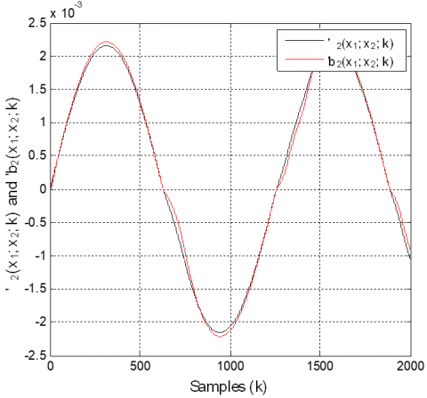
The parameter c1 in the Eq. (47) is given by -0.5, and the vector of the measurement noise $\mathbf{v}(k)$ is a zero mean independent random with variances, $R_{v 1}$ and $R_{v 2}$, fixed as 10-5. By running the simulation, $k_{1}, k_{2}$ and $\lambda_{2}$ for the control $\bar{u}_{a f b}(k)$ and $c_{v}$ for the SWLSE are chosen to provide better performances. The choice of the parameters values is as follows: $k_{1}=0.3, k_{2}=0.4, \lambda_{2}=0.25$ and $c_{v}=0.01$. The state variables evolutions of $x_{1}(k)$ and $x_{2}(k)$, and their estimates, $\hat{x}_{1}(k)$ and $\hat{x}_{2}(k)$, the nonlinear uncertainties, $\varphi_{1}\left(x_{1}, k\right)$ and $\varphi_{2}\left(x_{1}, x_{2}, k\right)$, and their estimates, and the proposed control are, shown, respectively, in the Figures 1-5.
Figures 1 and 2 show the evolutions of $x_{1}(k), \hat{x}_{1}(k), x_{2}(k)$ and $\hat{x}_{2}(k)$ which are bounded, and $\hat{x}_{1}(k)$ and $\hat{x}_{2}(k)$, approximate, $x_{1}(k)$ and $x_{2}(k)$ respectively. Figures 3 and 4 show that $\theta_{1}^{T}(k) \xi_{1}\left(\hat{x}_{1}\right)$ and $\theta_{2}^{T}(k) \xi_{2}\left(\hat{x}_{1}, \hat{x}_{2}\right)$ respectively, are close to $\varphi_{1}\left(x_{1}, k\right)$ and $\varphi_{2}\left(x_{1}, x_{2}, k\right)$. In Figure 5, we show that the evolution of the control signal is smooth and bounded. The effectiveness of the approach is shown by comparing the root mean squares obtained by the $\bar{u}_{a f b}(k)$ controller with those in [12] is given in the following Table 3:
Figure 1. Evolutions of $x_{1}(k)$ (black line) and its estimate $\hat{x}_{1}(k)$ (red line)
Figure 2. Evolutions of $x_{2}(k)$ (black line) and its estimate $\hat{x}_{2}(k)$ (red line)
Figure 3. Evolutions of $\varphi_{1}(k)$ (black line) and its estimate $\varphi_{1}(k)$ (red line)
Figure 4. Evolutions of $\varphi_{2}(k)$ (black line) and its estimate $\varphi_{2}(k)$ (red line)
Figure 5. Evolutions of the control signal
Table 3. Root mean squares of the variables
|
|
$x_{1}$ |
$x_{2}$ |
${\varepsilon_{1}\left(\widetilde{\varphi}_{1}\right)}$ |
${\varepsilon_{2}\left(\widetilde{\varphi}_{2}\right)}$ |
$\bar{u}_{a f b}$ |
|
Results in [12] |
0.0113 |
0.0086 |
0.0023 |
0.0019 |
0.0128 |
|
Our results |
0.0100 |
0.0044 |
0.0080 |
$1.68 \times 10^{-8}$ |
0.0033 |
The root mean squares of some signals are evaluated. comparing our results with those of [12], we can see that better tracking performance is obtained in this paper without chattering in the states and their estimates. as a conclusion, we can say from simulation, that the controller $\bar{u}_{a f b}(k)$ guarantee better performance without chattering, andthat the estimation errors, approach zero as time increases.
In this work, a novel hybrid interval type-2 fuzzy backstepping controller for a class of discrete-time nonlinear systems is proposed. A discrete-tile nonlinear equation with uncertainties describes the systems for which no mathematical model is available and some states are observed with measurement noises. The controller is calculated by taking out the issue of the complexity of computational burden. Estimation of the non-measurable states and adjustable parameters was performed. It has been proven that the boundedness of states under the controller action, and that the errors of estimation of the nonlinear functions remain around zero. The efficiency of the proposed controller has been demonstrated by performing the simulation results. We have applied the controller to discrete-time single input uncertain nonlinear systems. For future work, this controller will be extended to a class of uncertain discrete-time multi-input-multi-output nonlinear systems. Moreover, the controller based on the interval type-2 fuzzy systems discussed in Section 3will be studied in future work by combining this approach with neural network approach.
This work was supported by the Algerian Ministry of Higher Education and Scientific Research (MESRS) for PRFU Research Project No. A01L07UN280120200002.
[1] Chang, Y., Cheng, C.C. (2010). Block backstepping control of multi-input nonlinear systems with mismatched perturbations for asymptotic stability. International Journal of Control, 83(10): 2028-2039. https://doi.org/10.1080/00207179.2010.501869
[2] Krstić, M., Kanellakopoulos, I., Kokotović, P. (1992). Adaptive nonlinear control without over parametrization. Systems & Control Letters, 19(3): 177-185. https://doi.org/10.1016/0167-6911(92)90111-5
[3] Pan, Z., Basar, T. (1998). Adaptive controller design for tracking and disturbance attenuation in parametric strict-feedback nonlinear systems. IEEE Transactions on Automatic Control, 43(8): 1066-1083. https://doi.org/10.1109/9.704978
[4] Yao, B., Tomizuka, M. (2001). Adaptive robust control of MIMO nonlinear systems in semi-strict feedback forms. Automatica, 37(9): 1305-1321. http://dx.doi.org/10.1016/S0005-1098(01)00082-6
[5] Cheng, C.C., Ou, Y.H. (2013). Design of adaptive block backstepping controllers for uncertain nonlinear dynamic systems with n blocks. International Journal of Control, 86(3): 469-477. https://doi.org/10.1080/00207179.2012.739710
[6] Zeng, S., Pan, Z. (2009). Adaptive controller design and disturbance attenuation for SISO linear systems with noisy output measurements and partly measured disturbances. International Journal of Control, 82(2): 310-334. https://doi.org/10.1080/00207170802085011
[7] Yang, Z.J., Nagai, T., Kanae, S., Wada, K. (2007). Dynamic surface control approach to adaptive robust control of nonlinear systems in semi-strict feedback form. International Journal of Systems Science, 38(9): 709-724. https://doi.org/10.1080/00207720701596532
[8] Bendjaima, B., Saigaa, D., Khodja, D.E. (2017). Fault tolerant control based on adaptive fuzzy sliding mode controller for induction-motors. International Journal of Intelligent Engineering and Systems, 10(6): 39-48. http://dx.doi.org/10.22266/ijies2017.1231.05
[9] Khettab, K., Bensafia, Y., Ladaci, S. (2017). Chattering elimination in fuzzy sliding mode control of fractional chaotic systems using a fractional adaptive proportional integral controller. International Journal of Intelligent Engineering and Systems, 10(5): 255-266. https://doi.org/10.22266/IJIES2017.1031.28
[10] Lu, Y. (2018). Adaptive-fuzzy control compensation design for direct adaptive fuzzy control. IEEE Transactions on Fuzzy Systems, 26(6): 3222-3231. https://doi.org/10.1109/TFUZZ.2018.2815552
[11] Eini, R., Abdelwahed, S. (2019). Rotational inverted pendulum controller design using indirect adaptive fuzzy model predictive control. 2019 IEEE International Conference on Fuzzy Systems (FUZZ-IEEE), pp. 1-6. https://doi.org/10.1109/FUZZ-IEEE.2019.8859014
[12] Yoshimura, T. (2015). Design of a simplified adaptive fuzzy backstepping control for uncertain discrete-time nonlinear systems. International Journal of Systems Science, 46(5): 763-775. https://doi.org/10.1080/00207721.2014.973468
[13] Zeghlache, S., Ghellab, M.Z., Bouguerra, A. (2017). Adaptive type-2 fuzzy sliding mode control using supervisory type-2 fuzzy control for 6 DOF octorotor aircraft. International Journal of Intelligent Engineering and Systems, 10(3): 47-57. https://doi.org/10.22266/ijies2017.0630.06
[14] Khettab, K., Bensafia, Y., Ladaci, S. (2017). Robust adaptive interval type-2 fuzzy synchronization for a class of fractional order chaotic systems. In Fractional Order Control and Synchronization of Chaotic Systems, pp. 203-224. http://dx.doi.org/10.4018/978-1-5225-5418-9.ch004
[15] Wang, L.X. (1994). Adaptive Fuzzy Systems and Control: Design and Stability Analysis, Prentice-Hall, Inc.
[16] Rahali, H., Zeghlache, S., Benalia, L. (2017). Adaptive field-oriented control using supervisory type-2 fuzzy control for dual star induction machine. International Journal of Intelligent Engineering and Systems, 10(4): 28-40. http://dx.doi.org/10.22266/ijies2017.0831.04
[17] Li, Y.M., Yang, Y., Li, L. (2012). Adaptive backstepping fuzzy control based on type-2 fuzzy system. Journal of Applied Mathematics, pp. 1-27. http://dx.doi.org/10.1155/2012/658424
[18] Yoshimura, T. (2016). Design of an adaptive fuzzy sliding mode control for uncertain discrete-time nonlinear systems based on noisy measurements. International Journal of Systems Science, 47(3): 617-630. https://doi.org/10.1080/00207721.2014.891776
[19] Abdelmalki, F., Ouaaline, N. (2018). The fuzzy tracking control of output vector of double fed induction generator DFIG via T-S Fuzzy Model. International Journal of Intelligent Engineering and Systems, 11(1): 113-120.
[20] Tong, S.C., Li, Y.M., (2009). Observer-based fuzzy adaptive control for strict-feedback nonlinear systems. Fuzzy Sets and Systems, 160(12): 1749-1764. https://doi.org/10.1016/j.fss.2008.09.004
[21] Boudaraia, K., Mahmoudi, H., Abbou, A. (2019). MPPT design using artificial neural network and backstepping sliding mode approach for photovoltaic system under various weather conditions. International Journal of Intelligent Engineering and Systems, 12(6): 177-186. http://dx.doi.org/10.22266/ijies2019.1231.17
[22] El Idrissi, R., Abbou, A., Mokhlis, M. (2020). Backstepping integral sliding mode control method for maximum power point tracking for optimization of PV system operation based on high-gain observer. International Journal of Intelligent Engineering and Systems, 13(5): 133-144. https://doi.org/10.22266/ijies2020.1031.13
[23] Nafia, N., El Kari, A., Ayad, H., Mjahed, M. (2018). A robust type-2 fuzzy sliding mode controller for disturbed MIMO nonlinear systems with unknown dynamics. Journal for Control, Measurement, Electronics, Computing and Communications, 59(2): 194-207. http://dx.doi.org/10.1080/00051144.2018.1521568