Chahrazad Ogab* | Said Hassaine | Morsli Sbaa | Kamel Haddouche | Azeddine Bendiabdellah
© 2021 IIETA. This article is published by IIETA and is licensed under the CC BY 4.0 license (http://creativecommons.org/licenses/by/4.0/).
OPEN ACCESS
This article proposes a digital control strategy of the RST type combined with a PI regulator of a synchronous servomotor with permanent magnets supplied by a voltage inverter controlled by the vector PWM technique whose robustness of the regulators is studied by the µ-analysis technique, and the estimation of the mechanical quantities is carried out using an observer by the Kalman filter. This study presents a detailed theoretical analysis and the simulation and experimentation results obtained clearly show the effectiveness of the proposed control strategy.
PWM inverter, RST controller, PMSM, µ analysis, Kalman filter
The advantage of motor control is that the motor is a low-cost, low-density actuator in most industrial exercises. In industry, the speed transmission market seems to be developing, and the designer's wish is to achieve better performance of mechanical converter components [1-3]. However, controlling such a machine requires an accurate understanding of the position of the rotor, which provides its own driving. This information can be provided by mechanical sensors, which leads to some defects, including: increased volume, increased total system cost, and reduced system reliability. In addition, this requires a tree end that can be used to add sensors [4]. For all these reasons, intense research has been carried out since the 1980s in order to delete these clauses. Among the most common approaches are observer-based approaches such as the extended Kalman filter [5], linear or non-linear observers [6, 7], adaptive interconnected observers [8] or the observers by sliding modes [9].
Automatic control is called robust when certain characteristics, especially the actual stability and performance, do not deteriorate significantly when the process control model contains imprecision. For example, the ignored fast mode or important parameter error in the model [10]. It is possible to evaluate the uncertain stability only after the small gain theorem appears. The application of this method has become interesting after its popularity by µ-analysis, which allows parameter uncertainty, additional dynamics or noise to be included in the nominal model of the system to test its stability. Finally, the search for the minimum gain that destroys the stability of the system confirms or negates the stability of the system [11].
In this paper, the structure of the permanent magnet synchronous motor controller based on RST and PI is introduced. The experimental platform (Figure 1) has been installed in the industrial information and Automation Laboratory of Poitiers, France. It includes a DSPACE 1104 digital prototype card and its data acquisition interface, and a three-phase inverter based on IGBTs. It is controlled by vector Pulse Width Modulation (PWM) technology and a synchronous permanent magnet servo motor (PMSM) equipped with a resonator for angular position capture [12-14].
Figure 1. Photos of the test bench
In the following cases, the RST digital regulator is studied and a comparative study is made between the proposed control strategies using the PI cascade regulation studied and tested at [13, 14].
The stability analysis of the regulator is mainly to observe the behavior of speed and current when the PMSM parameters change. In order to make this analysis more rigorous, these variables are generated based on the study of [13, 14] and can only be applied after their impact on the stability of servo system has been studied by using µ-analysis technology. This technique will be briefly introduced to calculate structured unique values ("VSS") using Matlab toolbox [15]. However, we believe that in this study, there are only robust stability and parameter uncertainties. Then, observer is provided by Kalman filter to perform sensorless control [16, 17].
By considering the classical simplifying assumptions, the model of the synchronous machine in Park's reference frame can be given by the following system:
$\left\{\begin{array}{c}\frac{d}{d t} i_{d}=-\frac{R_{\mathrm{s}}}{L_{d}} i_{d}+\omega \frac{L_{q}}{L_{d}} i_{q}+\frac{1}{L_{d}} V_{d} \\ \frac{d}{d t} i_{q}=-\frac{R_{\mathrm{s}}}{L_{q}} i_{q}-\omega \frac{L_{d}}{L_{q}} i_{d}-\frac{\phi_{f}}{L_{q}} \omega+\frac{1}{L_{q}} V_{q} \\ \frac{d}{d t} \omega=\frac{p}{J}\left(T_{e}-T_{L}-B \omega\right) \\ T_{e}=p\left[\left(L_{d}-L_{q}\right) i_{d}+\phi_{f}\right] i_{q}\end{array}\right.$ (1)
The most common strategy for controlling the torque of this machine is to keep the id current at zero and to control the speed and / or position by the iq current through the Vq voltage [12-14]. When id current is zero, the simplified model of PMSM is provided by equation system (2).
$\left\{\begin{array}{l}V_{d}=-L_{q} \omega i_{q} \\ V_{q}=R_{s} i_{q}+L_{q} \frac{d}{d t} i_{q}+\omega \phi_{f} \\ T_{e}=p \phi_{f} i_{q} \\ \frac{d}{d t} \omega=\frac{p}{J}\left(T_{e}-T_{L}-B \omega\right)\end{array}\right.$ (2)
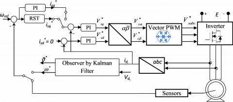
Therefore, the iq current that controls the torque developed by PMSM is generated by the speed regulator. We use the traditional PI corrector to generate the control signal on the voltage inverter arm. The structure of the current loop along the q axis with a PI corrector is represented by the diagram in Figure 2.
Figure 2. General block diagram of the control system
The parameters of the PI regulator are chosen in such a way that the zero introduced by the regulator is compensated by the dynamics of the current iq.
By modeling the inverter by a unity gain G0 = 1, we obtain:
$\frac{{{K}_{i{{i}_{q}}}}}{{{K}_{p{{i}_{q}}}}}=\frac{{{R}_{s}}}{{{L}_{q}}}$
The closed loop transfer function is given by:
$\frac{{{i}_{q}}}{i_{q}^{*}}=\frac{1}{{\scriptstyle{}^{{{L}_{q}}}/{}_{{{K}_{piq}}}}s+1}=\frac{1}{{{T}_{0}}s+1}$ (3)
T0: the dynamic imposed by the current loop.
Approaching the closed loop of the current by a first-order transfer function and for a zero-resistant torque, the open-loop transfer function of the system studied is based on the expression
$F(s)=\frac{p \phi_{f}}{J T_{0} s^{2}+\left(J+B T_{0}\right) s+B}$ (4)
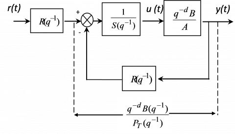
The inverter-PMSM association control strategy, proposed in this article, uses an RST structure based on pole placement. This structure is illustrated by the diagram in Figure 3. The pole placement algorithm is summarized as follows [12, 18]:
${{P}_{T}}({{q}^{-1}})=A({{q}^{-1}}) \,S({{q}^{-1}}) + {{q}^{-d}} \,B({{q}^{-1}}) \,R({{q}^{-1}})$ (5)
Figure 3. RST structure
We choose PT(q-1) in the form of a second order polynomial defined by its natural pulsation (w0) and it’s damping coefficient (z) while ensuring the following condition [12, 18]:
$0.25\le \,{{\omega }_{0}}{{T}_{s}}\le 1.5\,\,\,\,\,\,\,\,for\,\,\,\,\,\,\,0.7\le \zeta \le 1\,$ (6)
Note that the rules for automatic sampling frequency selection are as follows:
${{f}_{s}}=(6\,\,to\,\,25)\,f_{PB}^{CL}$ (7)
$\mathrm{f}_{\mathrm{PB}}^{\mathrm{CL}}$: Closed loop system bandwidth frequency.
And taking into account the switching frequency of the inverter, the sampling period is taken equal to Ts=100 μs. While the polynomial PT(q-1) is characterized by a damping coefficient ξ=0.7 and a natural pulsation ω0=3000 rad/s. After having chosen the polynomial PT(q-1), Eq. (5) allows obtaining the polynomials S and R. The polynomial T is given by [12, 18]:
$T({{q}^{-1}})=G\cdot {{P}_{T}}({{q}^{-1}})\,\,\text{with}\,\,G=\left\{ \begin{align} & \frac{1}{B(1)}\,\,\,\,if\,\,B(1)\ne 0 \\ & 1\,\,\,\,\,\,\,\,\,if\,\,B(1)=0 \\\end{align} \right.$ (8)
The discretization, with zero order blocker of the polynomial of the desired performances of the closed loop as well as the transfer function of the open loop of the system to be controlled, gives:
$\begin{align} & {{P}_{T}}({{q}^{-1}})={{p}_{2}}\,{{q}^{-2}}+{{p}_{1}}\,{{q}^{-1}}+1 \\ & \,\,\,\,\,\,\,\,\,\,\,\,\,\,\,\,\,\,\,=0.6570\,{{q}^{-2}}-1.5841\,{{q}^{-1}}+1 \\\end{align}$ (9)
$\begin{align} & F({{q}^{-1}})=\frac{B({{q}^{-1}})}{A({{q}^{-1}})}=\frac{{{b}_{1}}\,{{q}^{-1}}+{{b}_{2}}\,{{q}^{-2}}}{1+{{a}_{1}}\,{{q}^{-1}}+{{a}_{2}}\,{{q}^{-2}}} \\ & \,\,\,\,\,\,\,\,\,\,\,\,\,\,\,\,\,\,=\frac{\text{4}\text{.1831}{{\text{0}}^{\text{-04}}}{{q}^{-1}}+3.\text{9891}{{\text{0}}^{\text{-04}}}\,{{q}^{-2}}}{1-\text{1}\text{.867}\,{{q}^{-1}}+\text{0}\text{.867}\,{{q}^{-2}}} \\\end{align}$ (10)
3.1 Study of robustness using the μ-analysis technique
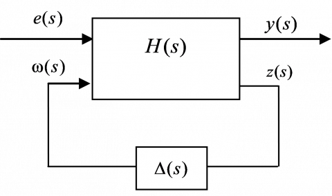
The principle of µ-analysis (Figure 4) is to evaluate a positive real $\bar{\mu}$, as small as possible and which is an upper bound of $\mu_{\Delta}\left(H_{z \omega}(j \omega)\right)$ on the imaginary axis. The usual procedure consists in choosing dense space of ω values. For each of these values, the upper bound of $\mu_{\Delta}\left(H_{z \omega}(j \omega)\right)$ is calculated using algorithms internal to Matlab [15, 19]. Then, the upper bound is assigned to $\bar{\mu}$. Thus, the robustness of the stability is ensured for any Δ(s) with norm H∞, less than or equal to $\bar{\mu}$. Each uncertain parameter is associated with an admissible interval. Let us recall that in the case of our study, this technique is only used to determine this interval [10, 11].
Figure 4. Formed into the Linear Fractional Transformation (LFT) uncertain process
3.2 Observation by Kalman filter
The Kalman filter is a state reconstruct or in a stochastic environment. It is an optimal state observer in the sense of minimizing the error variance between a real variable and it’s estimated. The Kalman filter is based on a stochastic linear state model [4, 20, 21].
$\left\{\begin{array}{c}X_{k+1}=A_{k} X_{k}+B_{k} U_{k}+W_{k} \\ Y_{k}=C_{k} X_{k}+V_{k}\end{array}\right.$ (11)
In this model, Xk represents the state vector, Uk the input vector and Yk. the measurement vector. The model is in fact a deterministic state model to which we add a state noise Wk, and a measurement noise Vk. These noises are assumed to be uncorrelated Gaussian white noises with zero mean [4, 22].
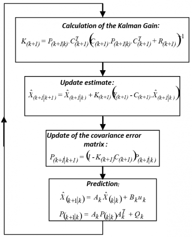
The Kalman filter is calculated in several steps using the procedure represented by the algorithm shown in Figure 5.
Figure 5. Steps of the algorithm of the recursive Kalman filter
The Kalman gain K is calculated to minimize the conditional variance of the error between the estimated state vector $\tilde{X}_{k}$ and the vector of real state Xk at time k, knowing the set of measurements at time k. Assuming that TL is identified, the fourth-order equations of state are:
$\left\{\begin{array}{l}{\left[\begin{array}{c}1_{\mathrm{d}} \\ \mathrm{l}_{\mathrm{q}} \\ \dot{\omega} \\ \dot{\Theta}\end{array}\right]=\left[\begin{array}{cccc}\frac{-R_{s}}{L_{d}} & \frac{\mathrm{L}_{\mathrm{q}}}{\mathrm{L}_{\mathrm{d}}} \omega & 0 & 0 \\ -\omega \frac{\mathrm{L}_{\mathrm{d}}}{\mathrm{L}_{\mathrm{q}}} & \frac{-R_{s}}{L_{q}} & \frac{-\phi_{f}}{L_{q}} & 0 \\ 0 & \frac{p \phi_{f}}{J} & \frac{-B}{J} & 0 \\ 0 & 0 & 1 & 0\end{array}\right]\left[\begin{array}{l}i_{d} \\ i_{q} \\ \omega \\ \Theta\end{array}\right]} \\ +\left[\begin{array}{ccc}\frac{1}{L_{d}} & 0 & 0 \\ 0 & \frac{1}{L_{q}} & 0 \\ 0 & 0 & \frac{-p}{J} \\ 0 & 0 & 0\end{array}\right]\left[\begin{array}{c}V_{d} \\ V_{q} \\ T_{L}\end{array}\right]\left[\begin{array}{c}I_{d} \\ I_{q}\end{array}\right]=\left[\begin{array}{llll}1 & 0 & 0 & 0 \\ 0 & 1 & 0 & 0\end{array}\right]\left[\begin{array}{c}I_{d} \\ I_{q} \\ \omega \\ \theta\end{array}\right]\end{array}\right.$
In our case, the discrete formulation of the Kalman filter consists first of all in carrying out a limited expansion in Taylor series of order 1 in order to be able to linearize the system, and taking into account, over a time interval Ts; that the speed is slowly variable but updated at each instant k.
By performing the 1st order discretization according to Euler, we obtain:
$\left[\begin{array}{l}I_{d_{k+1}} \\ I_{q_{k+1}} \\ \omega_{k+1} \\ \theta_{k+1}\end{array}\right]=\left[\begin{array}{cccc}\frac{1-T_{s} R_{s}}{L_{d}} & \mathrm{~T}_{\mathrm{s}} \frac{\mathrm{L}_{\mathrm{q}}}{\mathrm{L}_{\mathrm{d}}} \omega & 0 & 0 \\ -\mathrm{T}_{\mathrm{s}} \frac{\mathrm{L}_{\mathrm{d}}}{\mathrm{L}_{\mathrm{q}}} \omega & 1-\frac{T_{s} R_{s}}{L_{q}} & \frac{-T_{s} \phi_{f}}{L_{q}} & 0 \\ 0 & T_{s} \frac{p^{2} \phi_{f}}{J} & 1-\frac{T_{s} f_{c}}{J} & 0 \\ 0 & 0 & T_{s} & 1\end{array}\right]\left[\begin{array}{l}I_{d_{k}} \\ I_{q_{k}} \\ \omega_{k} \\ \theta_{\mathrm{k}}\end{array}\right]$
$+\left[\begin{array}{ccc}\frac{T_{s}}{L_{d}} & 0 & 0 \\ 0 & \frac{T_{s}}{L_{q}} & 0 \\ 0 & 0 & \frac{-T_{s}}{J} \\ 0 & 0 & 0\end{array}\right]\left[\begin{array}{c}V_{d_{k}} \\ V_{q_{k}} \\ T_{L_{k}}\end{array}\right]$
The use of the Kalman filter makes it possible to take into account a certain number of uncertainties which makes it relatively robust. However, its adjustment depends on the variance of the state noise and of the measurement noise, quantities which are relatively difficult to determine a priori, and which depend on the conditions of use.
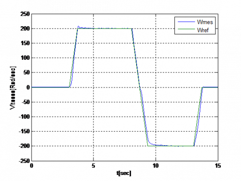
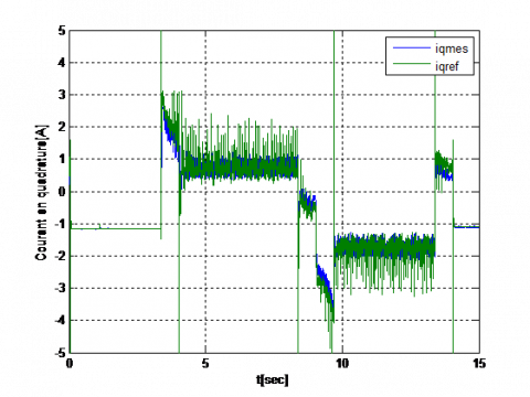
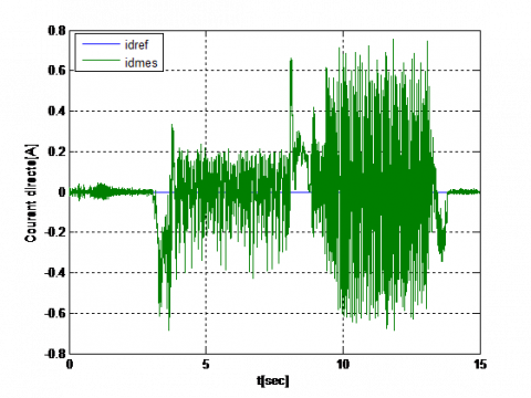
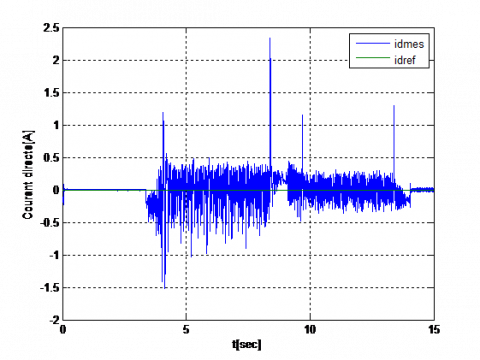
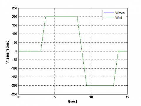
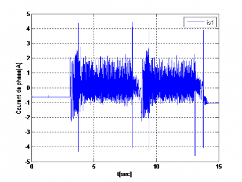
In what follows, we present the simulation and experimental curves of the evolution of the controlled speed, the images of the stator currents id and iq in the frame of reference (d, q), and finally, the last plot concerns the phase current. These results concern a speed benchmark varying from ± 200 rad / s, compared to the estimated speed, the difference between these two quantities is presented by the error of the speed following. Note that due to the safety of the equipment, the extreme values of the current iq are equal to ± 5A.
Figure 6. Experimental results- speed and current PI regulation
Figure 7. Experimental results- speed and current RST regulation
In Figures 6 and 7, we present the experimental results obtained by the studied control strategy, compared to a vector control strategy employing PI regulators of current and speed. Assuming that the internal current loop is approximated by unity gain and using the pole / zero compensation method, the PI speed regulator parameters are given by [13]:
$K_{p V}=0.06, K_{i V}=K_{p V} \frac{B}{J}$
We notice that the error of the speed following of the RST regulator is low whose maximum value during the change of set point is less than ± 0.2 rad / sec. In contrast, the tracking error for vector control reaches ± 30 rad / sec in transient. On the other hand, the direct current id presents peaks during the change of speed, in the case of the proposed control strategy, but this has no influence on the speed behavior of the motor.
The reference current along the q axis saturates at start-up and when changing the speed reference.
These same Figures 6, 7 illustrate the engine speed response when a resistive torque step is applied to it. This test clearly shows that the disturbance of the load has no effect on the behavior of the speed controlled by the digital regulator RST; on the other hand, the speed drop is more important when controlled by the PI regulator.
Recall that the application of the µ-analysis technique algorithm gave us the results presented in Table 1.
Table 1. The limits of variation of the parameters in percentage provided by the technique µ-analysis
|
|
Upper Bound |
Lower Bound |
Destabilizing Frequency |
|
Rsi |
1.0000 |
0.9997 |
10.4809 rad/s. |
|
Ji |
0.9999 |
0.987 |
0.0404 |
|
$\phi_{f i}$ |
Inf |
1.5499e+10 |
37777 rad/s. |
In order to test the robustness of the regulator, these variations will be introduced separately only in the parameter file. The results of Figure 8 clearly showed that this command effectively controls the effect of parametric variations. On the other hand, the shape of the currents was affected, in particular in the case of the variation of the moment of inertia; this obliges us to think of improving the current loop by using other regulators. In Figure 9, we present the simulation results obtained by associating the nonlinear state observer by Kalman filter with the regulation loop to estimate the speed of rotation and the position of the rotor. In order to implement the Kalman filter on the machine, it remains to choose the values of the initialization matrices P0, of state noise Qk=Q, and of measurement noise Rk=R. This problem is major to ensure the correct estimation of the position and the speed [4]. The adjustments of Q and R have been made to ensure stability throughout the speed range, while respecting a trade-off with dynamics and static errors. These settings are certainly not optimal, but the qualities of this filter ensure correct operation. The choice of the values of the initialization matrices, of state noise and of measurement noise, is carried out as follows:
$P_{0}=\left[\begin{array}{lcll}0.00001 & 0 & 0 & 0 \\ 0 & 0.00001 & 0 & 0 \\ 0 & 0 & 0.00001 & 0 \\ 0 & 0 & 0 & 0\end{array}\right]$
$Q=\left[\begin{array}{cccc}0.00001 & 0 & 0 & 0 \\ 0 & 0.00001 & 0 & 0 \\ 0 & 0 & 0.00001 & 0 \\ 0 & 0 & 0 & 0\end{array}\right]$
$R=\left[\begin{array}{cc}0.001 & 0 \\ 0 & 0.001\end{array}\right]$
Figure 8. Experimental results under variable: J (+100%)
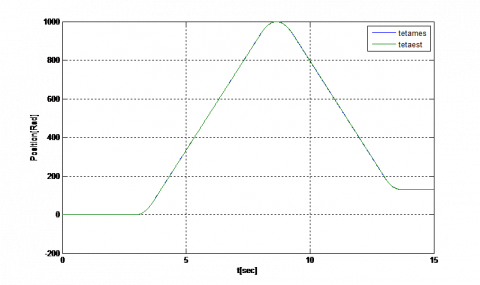
The machine being initially stopped, the initial state is zero; moreover, we assume the position error at start is zero. These results have shown the efficiency of this filter, they result in a low estimation error for different rotational speeds, as well as in the insensitivity to the parametric variation.
Figure 9. Simulation results RST associated with a Kalman filter: a) No load, b) under variable J (+ 100%)
In this work, a comparative study was carried out between a classical PI type vector control [13] and the proposed numerical control strategy. This study has shown the effectiveness and robustness of the latter.
The tracking error is very low, and the disturbance rejection is perfect. Note that the operating conditions of the two structures are identical, namely the test benchmark and the load torque applied. Regarding the digital structure in RST, the internal loop correctors (currents) have been retained. Thus, the proposed digital control structure has better dynamic performance compared to those obtained with conventional vector control in set point tracking and in disturbance rejection. The robustness tests, whose parametric variation used was studied by the µ-analysis technique, further proved the robustness of the RST regulator in monitoring the set point with respect to the parametric uncertainty, the influence of which was negligible. On the other hand, these same tests mentioned the need to improve the current loop in order to obtain a globally robust control strategy. The results obtained by simulation, of the control without position sensor, show the efficiency of the Kalman filter. They are characterized by a very small estimation error for different rotational speeds as well as by insensitivity to parameter variations.
The authors wish to thank all the team of the Laboratory of Automatic and Industrial Informatics of the University of Poitiers FRANCE and special thanks to Pr. Gerard Champenois for the aid he afforded us for the realization of our experimental work validation.
|
Vd, Vq |
Stator winding d, q axis voltages |
|
id, iq |
Stator winding d, q axis currents |
|
w |
Rotor speed |
|
wref |
Reference rotor speed |
|
θ |
Rotor position |
|
$\phi_{f}$ |
Constant magnet flux linkage produced by permanent magnet rotor |
|
$\phi_{d}, \phi_{a}$ |
Frame stator flux linkages |
|
Te |
Electromagnetic torque |
|
TL |
External load torque |
|
Ts |
Sampling period |
|
p |
Number of pole pairs |
|
Rs |
Stator resistance |
|
Ld, Lq |
Stator winding d, q -axis inductances |
|
J |
Inertia constant |
|
B |
Damping coefficient |
|
e(s) |
Controlled inputs |
|
w (s) |
disturbance input |
|
y (s) |
Controlled output |
|
z (s) |
disruption outputs |
|
Δ(s) |
Uncertainties on the system model |
|
H(s) |
nominal transfer of the closed loop system |
|
$\mu_{\Delta}$ |
The largest structured singular value (SSV) |
|
s |
Laplace operator |
|
Rs = 0.57 Ω |
|
Ld=4 mH |
|
Lq=4.5 mH |
|
Φf =0.064 Wb |
|
p=2 |
|
J=2.08. 10-3Kgm2 |
|
B=3.9.10-3Nm s/rad |
|
Rated speed =314 rad/s |
|
Nominal power =1 KW |
|
Rated torque =3 Nm |
[1] Abir, A., Mehdi, D. (2017). Control of permanent-magnet generators applied to variable-speed wind-energy. In 2017 International Conference on Green Energy Conversion Systems (GECS), pp. 1-6. https://doi.org/10.1109/GECS.2017.8066263
[2] Al-Toma, A.S., Taylor, G.A., Abbod, M. (2016). Development of space vector modulation control schemes for grid connected variable speed permanent magnet synchronous generator wind turbines. In 2016 51st International Universities Power Engineering Conference (UPEC), pp. 1-6. https://doi.org/10.1109/UPEC.2016.8114130
[3] Al-Toma, A.S., Taylor, G.A., Abbod, M., Pisica, I. (2017). A comparison of PI and fuzzy logic control schemes for field oriented permanent magnet synchronous generator wind turbines. In 2017 IEEE PES Innovative Smart Grid Technologies Conference Europe (ISGT-Europe), pp. 1-6. https://doi.org/10.1109/ISGTEurope.2017.8260331
[4] de Fornel, B., Louis, J.P. (Eds.). (2007). Identification et observation des actionneurs électriques: Exemples d'observateurs. Lavoisier.
[5] Bendjedia, M., Ait-Amirat, Y., Walther, B., Berthon, A. (2011). Position control of a sensorless stepper motor. IEEE Transactions on Power Electronics, 27(2): 578-587. https://doi.org/10.1109/TPEL.2011.2161774
[6] Rizvi, S.A.A., Memon, A.Y. (2019). An extended observer-based robust nonlinear speed sensorless controller for a PMSM. International Journal of Control, 92(9): 2123-2135. https://doi.org/10.1080/00207179.2018.1428768
[7] Ortega, R., Praly, L., Astolfi, A., Lee, J., Nam, K. (2010). Estimation of rotor position and speed of permanent magnet synchronous motors with guaranteed stability. IEEE Transactions on Control Systems Technology, 19(3): 601-614. https://doi.org/10.1109/TCST.2010.2047396
[8] Hamida, M. A., De Leon, J., Glumineau, A., Boisliveau, R. (2012). An adaptive interconnected observer for sensorless control of PM synchronous motors with online parameter identification. IEEE Transactions on Industrial Electronics, 60(2): 739-748. https://doi.org/10.1109/TIE.2012.2206355
[9] Kim, H., Son, J., Lee, J. (2010). A high-speed sliding-mode observer for the sensorless speed control of a PMSM. IEEE Transactions on Industrial Electronics, 58(9): 4069-4077. 10.1109/TIE.2010.2098357
[10] Duc, G., Font, S. (1999). Commande H∞ et μ-analyse. Hermes Sciences Publication.
[11] Lesprier, J., Roos, C., Biannic, J.M. (2015). Improved μ upper bound computation using the μ-sensitivities. IFAC-PapersOnLine, 48(14): 215-220. https://doi.org/10.1016/j.ifacol.2015.09.460
[12] Ogab, C. Bendiabdellah, A. Moreau, S. Hassaine, S. (2009). An RST numerical applied to a permanent magnet synchronous machine. International Review of Electrical Engineering, 4(3): 461-469.
[13] Hassaine, S., Moreau, S., Ogab, C., Mazari, B. (2007). Robust speed control of PMSM using generalized predictive and direct torque control techniques. In 2007 IEEE International Symposium on Industrial Electronics, pp. 1213-1218. https://doi.org/10.1109/ISIE.2007.4374771
[14] Longchamp, R. (2010). Commande numérique de systèmes dynamiques: Cours d'automatique, 1. PPUR Presses polytechniques.
[15] Balas, G.J., Doyle, J.C., Glover, K., Packard, A., Smith, R. (1995). µ-Analysis and synthesis toolbox user’s guide. The MathWorks, Natick, MA, version, 3.
[16] Almarhoon, A.H., Zhu, Z.Q., Xu, P. (2016). Improved rotor position estimation accuracy by rotating carrier signal injection utilizing zero-sequence carrier voltage for dual three-phase PMSM. IEEE Transactions on Industrial Electronics, 64(6): 4454-4462. https://doi.org/10.1109/TIE.2016.2561261
[17] Trancho, E., Ibarra, E., Arias, A., Salazar, C., Lopez, I., de Guerenu, A. D., Peña, A. (2016). A novel PMSM hybrid sensorless control strategy for EV applications based on PLL and HFI. In IECON 2016-42nd Annual Conference of the IEEE Industrial Electronics Society, pp. 6669-6674. https://doi.org/10.1109/IECON.2016.7793330
[18] Sebaa, M., Hassaine, S., Ogab, C. (2017). Robust control method for PMSM based on internal model control with speed and load torque estimator. International Journal on Electrical Engineering and Informatics, 9(3): 493-503. https://doi.org/10.15676/ijeei.2017.9.3.6
[19] Popescu, D., Gharbi, A., Stefanoiu, D., Borne, P. (2017). Process Control Design for Industrial Applications. ISTE, Limited. https://doi.org/10.1002/9781119407461
[20] Soares, E.L., Rocha, F.V., de Siqueira, L.M.S., Rocha, N. (2018). Sensorless rotor position detection of doubly-fed induction generators for wind energy applications. In 2018 13th IEEE International Conference on Industry Applications (INDUSCON), pp. 1045-1050. https://doi.org/10.1109/INDUSCON.2018.8627227
[21] Xing, N., Xia, J., Cao, W., Lin, Z., Gadoue, S. (2019). A sensorless and adaptive control strategy for a wind turbine based on the surface-mounted permanent magnet synchronous generator and PWM-CSC. In 2019 26th International Workshop on Electric Drives: Improvement in Efficiency of Electric Drives (IWED), pp. 1-6. https://doi.org/10.1109/IWED.2019.8664302
[22] Rahmani, S., Ktata, S., Yeferni, K., Doub, F., Hamadi, A., Al-Haddad, K. (2019). A nonlinear control of PMSG based variable speed wind energy generation system connected to the grid. In 2019 19th International Conference on Sciences and Techniques of Automatic Control and Computer Engineering (STA), pp. 449-454. https://doi.org/10.1109/STA.2019.8717305