Andi Ridwan Makkulawu*![]() | Karma
| Karma![]() | Arwini Arisandi
| Arwini Arisandi![]() | Ismail Gaffar
| Ismail Gaffar![]()
© 2025 The authors. This article is published by IIETA and is licensed under the CC BY 4.0 license (http://creativecommons.org/licenses/by/4.0/).
OPEN ACCESS
The fisheries sector is vital for food security but remains vulnerable to supply fluctuations and uncertain stock availability. This study develops a forecasting framework for buffer stock estimation by applying the Autoregressive Integrated Moving Average (ARIMA) and Fuzzy Time Series Markov-Chain (FTS-MC) approaches to historical data from Makassar City, Indonesia during 2021–2025. The ARIMA (2,1,0) model produced acceptable accuracy with a Mean Absolute Percentage Error (MAPE) of 13.67%, whereas the FTS-MC method delivered superior outcomes with reduced errors (MAPE 10.91% and RMSE 246.94). These findings confirm the capability of FTS-MC in addressing volatility and uncertainty, offering more dependable projections of raw material reserves. The study provides practical implications for enhancing fisheries governance, stabilizing market distribution, and supporting strategic planning. Future research should incorporate broader datasets, real-time observations, and environmental parameters to refine predictive performance across varied contexts.
ARIMA, buffer stock, fisheries management, fuzzy time series Markov-Chain, MAPE, supply chain stability, time series analysis
The fishing industry in Indonesia plays a vital role in the national economy, contributing significantly to food security and providing livelihoods for millions of individuals across coastal communities. In recent years, Indonesia has become one of the world's largest exporters of fishery products, ranking eighth globally in 2020, despite the challenges posed by the COVID-19 pandemic [1]. The country's diverse marine ecosystem offers a plethora of aquatic resources, including various species of fish, crustaceans, and mollusk, which are essential for both domestic consumption and export markets. However, the rapid expansion of the fishing sector has also led to increased pressure on fish stocks, necessitating effective management strategies to sustain its long-term viability.
One of the primary challenges facing the Indonesian fishing industry is the issue of illegal, unreported, and unregulated (IUU) fishing, which jeopardizes marine biodiversity and undermines efforts to manage fisheries sustainably [2, 3]. With a vast archipelagic coastline, Indonesia is particularly vulnerable to IUU fishing practices that deplete fish stocks beyond sustainable levels. Moreover, overfishing exacerbates this problem, posing serious threats to marine ecosystems and the livelihoods of local fishermen. The government has been working to strengthen regulations and enforcement measures to combat IUU fishing, but substantial challenges remain in addressing this complex issue, including the need for international cooperation and improved surveillance capabilities [2, 3].
Another significant challenge lies in adapting to changes resulting from climate change. Fluctuations in ocean temperature, rising sea levels, and altered fish migration patterns have placed additional strain on the fishing industry, which must constantly adjust its practices to respond to these environmental shifts [4]. The impacts of climate change not only threaten fish stocks but also affect the communities that depend on fishing for their economic sustenance. To navigate these challenges effectively, the industry must adopt sustainable practices, enhance technological capacities, and invest in alternative livelihoods for affected communities. This transition is crucial to ensure the resilience of Indonesia's fishing industry against both immediate and long-term threats.
Buffer stocks serve as a crucial element in managing the volatility of fish supply and prices, particularly in Indonesia, a nation renowned for its extensive fishing resources. The primary role of buffer stocks is to stabilize fish markets by ensuring availability during periods of scarcity that may arise due to overfishing, seasonal catch variations, or environmental changes. This becomes increasingly important in Indonesia, where food security is a pressing concern amid rising population demands and fluctuating fish stocks [5]. The government’s strategic interventions via buffer stock schemes not only maintain equilibrium in prices but also protect low-income fishing communities from the adverse effects of market volatility [6]. By having a readily available reserve, fisheries can mitigate the risks associated with sudden supply shocks, thereby promoting sustainability and the economic welfare of fishing communities.
Moreover, buffer stocks contribute to long-term environmental sustainability in the fishing sector. By regulating catch limits through managed stocks, buffer systems can help prevent overfishing and allow fish populations to recover naturally. This approach is vital in Indonesia, where ecological balance is threatened by factors such as climate change and habitat degradation [7]. Additionally, effective buffer stock management fosters collaborative governance among stakeholders, ensuring that both governmental and local community interests align in sustainable fishing practices. Investments in buffer stock initiatives thus not only stabilize food supplies but also enhance social equity among fishing communities, ultimately contributing to improved livelihoods and environmental health [8]. In this context, buffer stocks play an indispensable role in securing the future of Indonesia's fishing industry whilst advancing broader socio-economic objectives.
Forecasting tools and methods in fisheries management play a critical role in ensuring sustainable practices that accommodate environmental variability and economic demands. One widely acknowledged methodology is the Autoregressive Integrated Moving Average (ARIMA) model, which has been effectively employed in predicting future fish stock levels and catch dynamics. Recent studies have indicated that integrating environmental covariates into ARIMA models, such as ocean temperature, enhances forecast accuracy regarding fish recruitment and productivity [9]. For instance, Porreca [10] demonstrates how ocean temperature forecasts can shape effort allocation in tuna fisheries, indicating the substantial impact of climatic factors on fishery outputs. This evolution of forecasting practices emphasizes the necessity for advanced statistical approaches that allow fisheries managers to make informed decisions amid variable environmental conditions [10].
In addition to ARIMA, the use of fuzzy time series and machine learning techniques is gaining traction in fisheries science, providing alternative approaches that can account for the inherent uncertainties present in ecological systems. For example, the amalgamation of genomic data with species distribution modeling positions fisheries management to adopt a more holistic view of stock assessments and environmental interactions [11]. As highlighted by study [12], forecasting systems designed to account for climate variability can enhance the understanding of species dynamics, particularly for species like squid, which are affected by fluctuating ocean conditions. Furthermore, innovative assessments that combine traditional ecological forecasting with contemporary modeling tools offer increased predictive power, leading to better resource management and sustainability strategies [13]. These advancements herald a new era of fisheries management, where data-driven approaches equipped with robust forecasting methodologies can directly inform conservation efforts while optimizing fishery outputs.
One of the primary challenges in forecasting fish stock dynamics is the insufficient predictive accuracy of existing methods. Traditional time series models, such as ARIMA, have been widely employed for their ability to analyze historical data and provide forecasts based on underlying patterns and seasonality. However, significant shortcomings arise when these models are applied to volatile systems like fisheries, where various external factors, such as environmental changes and market demand fluctuations, significantly influence stock levels. Research has indicated that ARIMA may yield low accuracy under conditions of high variability, leading to potentially misguided management strategies [14]. Furthermore, its dependency on historical linear relationships can overlook emerging trends, resulting in forecasts that fail to accurately capture the state of the fishery and its future dynamics. These limitations highlight a clear research gap in fisheries forecasting: conventional ARIMA models are not sufficiently capable of capturing the complex, non-linear, and uncertain behavior of fish stock systems. Addressing this gap requires forecasting techniques that explicitly incorporate uncertainty and variability.
In addition to predictive accuracy issues, there are inherent challenges associated with modeling complex systems such as the fishing industry. The dynamics of fish populations are influenced by a multitude of interrelated factors, including climatic variations, ecological interactions, and socio-economic forces. These complexities often elude simplistic modeling approaches, leading to inadequate predictions and ultimately ineffective fisheries management practices [15]. The integration of fuzzy logic with traditional forecasting models, such as the Fuzzy Time Series (FTS) Markov Chain, has shown promise in accommodating uncertainties and providing a more robust framework for prediction. However, this approach also faces its own challenges, such as the need for effective fuzzification and defuzzification processes, which can introduce additional uncertainty and affect the overall forecasting accuracy [16].
The implementation of such models entails extensive computational resources and a deep understanding of the underlying processes governing dynamic interactions, significantly complicating the modeling efforts. It is crucial for further research to explore hybrid methodologies that can dynamically adjust to changing conditions and provide accurate forecasts within complex, real-world contexts [17]. Furthermore, literature highlights the necessity for continuous adaptation of methodologies within fisheries management to effectively account for the multifaceted nature of the ecological and economic environments [18]. As fisheries increasingly confront challenges from climate change and human activity, enhancing the predictability of buffer stock models remains an urgent priority for sustainable resource management.
In this study, the primary objective is to design an integrated forecasting model for buffer stock management in the fishing industry, leveraging the strengths of the Autoregressive Integrated Moving Average (ARIMA) and fuzzy time series methods. By combining these methodologies, the proposed model aims to provide a more nuanced forecasting capability that accommodates the inherent uncertainties and complexities of fish stock dynamics. The ARIMA model offers a robust statistical framework for analyzing time series data, enabling accurate predictions based on historical trends [19]. On the other hand, fuzzy time series methods incorporate subjective judgments and uncertainties into the forecasting process, enhancing the model's adaptability to changing environmental and market conditions. The integration of these approaches is anticipated to create a comprehensive tool that enhances decision-making processes for fishery managers by yielding more reliable forecasts of buffer stock levels under various scenarios [13].
The second research objective is to assess the effectiveness of the integrated forecasting model in accurately predicting fish stock levels and improving management outcomes. Evaluating the model's performance involves comparing its forecasts against actual fish landings and stock assessments over a specified timeframe. This assessment will be conducted using statistical metrics such as Mean Absolute Percentage Error (MAPE) and Root Mean Square Error (RMSE) to gauge the accuracy and reliability of the predictions [20]. By conducting these assessments, the study seeks not only to validate the model's efficacy but also to explore its applicability across different fishing contexts and ecological settings. A successful model will provide stakeholders within the fishing industry with a tool to enhance adaptive management strategies, improve resource allocation, and ultimately contribute to the sustainability of fish stocks [21].
Furthermore, this research will also emphasize the importance of real-time data integration and environmental monitoring in enhancing the forecasting capabilities of the proposed model. By incorporating environmental variables and socio-economic factors, the forecasting model is expected to provide a more holistic view of the factors affecting fish stock dynamics [21]. This comprehensive approach ensures that forecasts are not only statistically sound but also contextually relevant, allowing fishery managers to respond effectively to real-world challenges faced by the industry. Overall, the primary goals of this research are to innovate in forecasting methodologies specific to the fishing industry and to create actionable, data-driven insights that bolster sustainable fishing practices.
The significance of this study lies in its relevance to sustainable fisheries management and the practical applications of the developed forecasting model using ARIMA and fuzzy time series Markov-Chain methods. With the increasing pressures of climate change and overfishing, effective management strategies must be rooted in robust scientific forecasting to ensure the long-term viability of fish stocks [10]. By integrating ARIMA and fuzzy time series Markov-Chain approaches, this study aims to provide refined predictions that consider the inherent uncertainties and complexities of fishery dynamics, thereby supporting efforts to maintain sustainable catches and prevent overexploitation [22]. The practical implementation of this predictive model holds substantial potential for informing policy development and enhancing resource management within the fisheries sector.
The research design for this study centers around a modeling approach that aims to forecast buffer stock levels in the fishing industry using ARIMA and fuzzy time series Markov-Chain methods. This approach effectively merges statistical rigor with adaptability to fisheries management uncertainties, supporting the goal of delivering precise, practical insights for sustainability. The conceptual framework underpinning this study draws from dynamic system theory, where the interactions between ecological variables (such as fish populations and environmental changes) and socio-economic factors (such as market demands and regulatory policies) are modeled to capture the complexity of fisheries dynamics [23, 24]. By applying this approach, the study seeks to contribute to policy-making and resource management in the fishing industry, facilitating the development of strategies that optimize both ecological resilience and economic viability for communities reliant on fisheries [10, 25].
This study was conducted in the fishing industry of Makassar City, South Sulawesi, from 2021 to 2025. The location was selected as it represents one of the largest fishing hubs in Eastern Indonesia, playing a strategic role in the seafood supply chain, and exhibiting ecosystem characteristics and fishing dynamics representative of tropical coastal fisheries. Secondary data were obtained from fishing companies using a purposive non-probability sampling approach to ensure that the selected sample captured specific characteristics relevant to the research objectives, including commodity types and the availability of historical raw material inventory data.
Sample selection followed the inclusion criteria of: (1) fishing companies operating within Makassar City; (2) possessing continuous historical records of at least 70 observations for the primary variables during 2021–2025; and (3) providing key observational variables, including inventory data and observation dates. The ≥70 observation threshold was adopted following [26], which recommends a minimum of 50-70 observations in time series analysis to ensure parameter stability and predictive accuracy. This requirement is also supported by fisheries-related forecasting studies, such as the studies [9, 19], which emphasize that sufficient sample sizes are critical to improve robustness and reduce forecasting errors in ecological and fisheries applications.
The analytical framework of this study is grounded in a statistical modeling approach combined with machine learning techniques, selected for their capability to capture temporal patterns and non-linear relationships in fisheries raw material inventory data. Model development was informed by theoretical concepts drawn from the literature on time-series analysis and predictive modeling, under assumptions including data stationarity, residual independence, and consistency of input variables throughout the observation period. Data analysis was conducted using Minitab Statistical Software 22 and RStudio with the R programming language (version 4.4.2), employing methods such as ARIMA and fuzzy time series based on the Markov Chain. Model performance was evaluated using the Mean Absolute Percentage Error (MAPE) and Root Mean Square Error (RMSE) to assess predictive accuracy. Statistical significance was assessed using 95% confidence intervals and a significance threshold of p < 0.05.
Historical time series data relevant to the analysis were compiled, including variables such as raw material inventory levels and measurement times. The ARIMA method was then applied to analyze the data, following the structured sequence of steps outlined below.
The AR component models the current value of a time series as a weighted sum of its previous values plus a stochastic error term. The general form of an AR(p) model is (Eq. (1)):
$y_t=c+\phi_1 y_{t-1}+\phi_2 y_{t-2}+\cdots+\phi_p y_{t-p}+e_t$ (1)
where, $c$ is a constant, $e_t$ is the error term, and $y_{t-1}, y_{t-2}, \ldots$, $y_{t-p}$ are past observations.
The I component addresses non-stationarity in the data by differencing the series $d$ times, removing trends and stabilizing the mean.
The MA component captures the linear dependence between the current observation and a finite number of past forecast errors. An MA$(q)$ process is expressed as Eq. (2):
$x_t=\mu+\phi_1 w_{t-1}+\phi_2 w_{t-2}+\cdots+\phi_p w_{t-p}+w_t$ (2)
where, μ is the mean of the series and $w_t$ is the white noise.
The complete ARIMA model combines these elements into (Eq. (3)):
$\begin{gathered}y=c+\phi_1 y_{t-1}+\cdots+\phi_p y_{t-p}+\mu-\phi_1 w_{t-1}-\cdots -\phi_p w_{t-q}+w_t\end{gathered}$ (3)
with p indicating the AR order, d the differencing order, and $q$ the MA order.
Fuzzy Time Series Markov Chain (FTS-MC) integrates the Fuzzy Time Series approach with the Markov Chain framework, utilizing a transition matrix to determine the highest probability and thereby achieve greater accuracy compared to the conventional Fuzzy Time Series method. The FTS-MC method employs the following algorithm, as described by studies [34, 35].
$\mu_{i j}=\left\{\begin{array}{cc}1, & i=1 \\ 0.5, & j=i-1 \text { or } j=i+1 \\ 0, & \text { otherwise }\end{array}\right.$ (4)
Each fuzzy set is expressed as (Eq. (5)):
$A_i=\left(\frac{\mu_{i 1}}{u_1}, \frac{\mu_{i 2}}{u_2}, \ldots, \frac{\mu_{i n}}{u_n}\right), \quad i=1,2, \ldots, n$ (5)
This approach assigns a full membership value of 1 to the central element, a partial membership value of 0.5 to its neighboring elements, and zero to all others, thereby preserving local relationships among data points and ensuring a structured, consistent representation for forecasting models.
$P_{i j}=\left[\begin{array}{cccc}p_{11} & p_{12} & \cdots & p_{1 n} \\ p_{21} & p_{22} & \cdots & p_{2 n} \\ \vdots & \vdots & \ddots & \vdots \\ p_{n 1} & p_{n 2} & \cdots & p_{n n}\end{array}\right]$ (6)
The forecasting process using the FTS-MC model consists of three main stages:
At time $t$, when the data belong to state $A_i$, the initial forecast is determined as follows:
Rule 1. If $A_i \rightarrow \emptyset$, then the forecast equals the midpoint of interval $u_i: F(t)=m_i$
Rule 2. If $A_i \rightarrow A_k$ with a unique transition, the forecast equals the midpoint of $u_k: F(t)=m_k$
Rule 3. If $A_i \rightarrow A_1, A_2, \ldots, A_n$, then the forecast is a weighted sum of the midpoints based on transition probabilities: $\quad F(t)=m_1 p_{i 1}+m_2 p_{i 2}+\cdots+m_{j-1} p_{i, j-1}+ Y(t-1) p_{i, j}+m_{j+1} p_{i, j+1}+\cdots+m_n \quad$ where $\quad m_j \quad$ is the midpoint of interval $u_j$, and $p_{i, j}$ denotes the transition probability from state $i$ to state $j$.
To improve accuracy, adjustment values are introduced according to the direction and step size of the transition:
Rule 1. Upward transition $(i<j): D_{t 1}=\frac{L}{2}$
Rule 2. Downward transition $(i>j): D_{t 1}=-\frac{L}{2}$
Rule 3. Forward shift by $s$ states $(i \rightarrow i+s): D_{t 2}=\left(\frac{L}{2}\right) s$
Rule 4. Backward shift by v states $(i \rightarrow i-v): D_{t 2}= -\left(\frac{L}{2}\right) v$
where, L is the interval length.
The final forecast value is obtained by correcting the initial forecast with the adjustment values (Eq. (7)):
$F^*(t)=F(t) \pm D_{t 1} \pm D_{t 2}$ (7)
Model validation is conducted to evaluate the predictive performance of the ARIMA and FTS-MC model by comparing its forecasts against a hold-out sample of historical data excluded from the model fitting process. This approach ensures that the assessment reflects the model’s ability to generalize beyond the training dataset. A commonly used performance metric is the MAPE, defined as Eq. (8):
$M A P E=\frac{100 \%}{n} \sum_{t=1}^n\left|\frac{y_t-\hat{y}_t}{y_t}\right|$ (8)
where, $y_t$ denotes the actual observed value at time $t$, $\hat{y}_t$ is the forecasted value, and $n$ represents the number of observations in the validation set. Lower MAPE values indicate better forecasting accuracy, with values below $10 \%$ generally considered highly accurate in many practical applications [36].
In addition to using the MAPE, the performance of a model can also be evaluated through the RMSE. RMSE provides information about the average magnitude of prediction errors in the same units as the measured variable, thereby facilitating the interpretation of model performance. A smaller RMSE value indicates better model accuracy and is mathematically expressed as Eq. (9):
$R M S E=\sqrt{\frac{1}{n} \sum_{t=1}^n\left(y_t-\hat{y}_t\right)^2}$ (9)
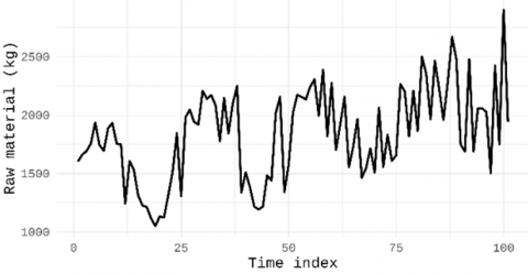
The following time series data illustrate weekly observations collected from early 2022 to 2024. To better understand the characteristics of the dataset, descriptive statistical analysis was conducted to examine measures of central tendency and data dispersion. The overall data pattern is visualized in Figure 1.
Figure 1 illustrates the time series data from 2022 onward, consisting of 101 weekly observations. The series has a mean of approximately 1,836, which is close to the median of 1,843, indicating a relatively balanced distribution. The values range between 1,050 and 2,900, reflecting considerable variability, with a standard deviation of 388.685. The skewness value of 0.036 suggests an almost symmetric distribution, with no pronounced deviation to either side. However, symmetry in distribution does not necessarily imply linearity in the time series behavior. The dataset may still exhibit non-linear dynamics, underscoring the need for forecasting methods capable of addressing both linear and non-linear patterns. Several upward peaks above 2,500 and downward troughs below 1,500 further highlight the pronounced fluctuations over time. Prior to ARIMA modeling, the data were tested for stationarity to ensure the appropriateness of the model specification.
Figure 1. Time series plot
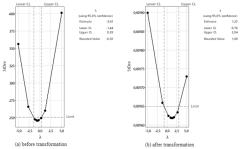
Figure 2. Box-Cox transformation
Figure 2 illustrates the Box-Cox transformation, where (a) shows the distribution before transformation and (b) after transformation. Prior to transformation, the rounded value of lambda (λ) was approximately −0.50, indicating the need for variance stabilization. After applying the Box-Cox transformation, the λ = 1, suggesting that the variance of the series had been stabilized and achieved stationarity. Subsequently, the stationarity of the mean was examined using the ADF test to further validate the adequacy of the transformation for time series modeling. The result showed a p = 0.169, indicating that the series was not yet stationary with respect to the mean. Therefore, first-order differencing was applied, after which the ADF test yielded a p = 0.000. This confirmed that the differenced series had achieved stationarity in the mean. Following this, model identification was conducted through the inspection of the ACF and PACF plots.
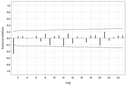
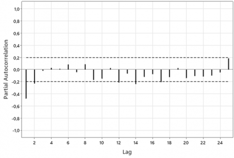
Based on Figure 3, the ACF plot exhibits a cut-off at lag 1, while the PACF plot shows a cut-off at lags 1 and 2. This indicates potential autoregressive parameters $p=1,2$ and a moving average parameter $q=1$. Consequently, tentative models were constructed with differencing order $d=1$, resulting in the following ARIMA specifications: ARIMA(0,1,1), ARIMA(1,1,0), ARIMA(1,1,1), ARIMA(2,1,0), and ARIMA(2,1,1).
Figure 3. ACF and PACF plot
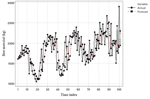
Following the estimation of tentative models, diagnostic checking was performed to validate model adequacy. This involved examining the residuals to ensure they exhibited white noise characteristics, namely a mean close to zero and the absence of significant autocorrelation. The Ljung–Box test confirmed the independence of residuals, indicating that the ARIMA(2,1,0) model satisfied the diagnostic criteria with p > 0.05. Consequently, ARIMA(2,1,0) was selected as the most suitable model for the series. The model was then applied to the time series data for forecasting to evaluate its performance and predictive accuracy, with the results presented in Figure 4.
Figure 4. Comparison between actual and forecast values using the ARIMA(2,1,0) model
The ARIMA(2,1,0) model achieved an RMSE of 314.79 and a MAPE of 13.67%, corresponding to an accuracy of 86.33%. As illustrated in Figure 4, the forecasted values closely followed the actual series, capturing both trend and fluctuations. Although the MAPE is slightly above the <10% threshold typically regarded as highly accurate, the results still demonstrate that the model provides a reliable level of forecasting accuracy. These results were then compared with the FTS-MC model to determine the most suitable model for time series forecasting.
The first step in FTS-MC modeling involves defining the universe of discourse based on the available data. In this study, the number of intervals $(k)$ was set to 7, with a minimum value of 1,050, a maximum value of 2,900, and an interval width of 264.29. The corresponding fuzzy intervals are summarized in Table 1.
Table 1. Fuzzy intervals
|
Interval |
Lower |
Upper |
Midpoint |
|
[1,050 – 1,314.29] |
1,050 |
1,314.29 |
1,182.14 |
|
[1,314.29 – 1,578.57] |
1,314.29 |
1,578.57 |
1,446.43 |
|
[1,578.57 – 1,842.86] |
1,578.57 |
1,842.86 |
1,710.71 |
|
[1,842.86 – 2,107.14] |
1,842.86 |
2,107.14 |
1975 |
|
[2,107.14 – 2,371.43] |
2,107.14 |
2,371.43 |
2,239.29 |
|
[2,371.43 – 2,635.71] |
2,371.43 |
2,635.71 |
2,503.57 |
|
[2,635.71 – 2,900] |
2,635.71 |
2,900 |
2,767.86 |
Next, the fuzzification process was performed to transform the actual data into fuzzy sets. This step allowed the identification of FLR between consecutive observations. The resulting FLRs are presented in Table 2.
Table 2. FLR result
|
$\boldsymbol{t}$ |
$y_t$ |
$state_t$ |
$y_{t+1}$ |
$state_{\text {t }+1}$ |
FLR |
|
1 |
1,602.637 |
3 |
1,661.886 |
3 |
$A_3 \rightarrow A_3$ |
|
2 |
1,661.886 |
3 |
1,692.556 |
3 |
$A_3 \rightarrow A_3$ |
|
3 |
1,692.556 |
3 |
1,757.069 |
3 |
$A_3 \rightarrow A_3$ |
|
$\vdots$ |
$\vdots$ |
$\vdots$ |
$\vdots$ |
$\vdots$ |
$\vdots$ |
|
98 |
2424.743 |
6 |
1750.970 |
3 |
$A_6 \rightarrow A_3$ |
|
99 |
1750.970 |
3 |
2900 |
7 |
$A_3 \rightarrow A_7$ |
|
100 |
2900 |
7 |
1943,849 |
4 |
$A_7 \rightarrow A_4$ |
Table 2 shows the Fuzzy Logical Relationship (FLR) results, which illustrate the transitions between fuzzy states over time based on historical data. These transitions form the basis for constructing the FLRG, which are summarized in Table 3.
Table 3. FLRG result
|
Current State |
Next State |
Total State |
|
$A_1$ |
$7\left(A_1\right), 3\left(A_4\right), 2\left(A_2\right), 1\left(A_3\right)$ |
13 |
|
$A_2$ |
$4\left(A_4\right), 4\left(A_3\right), 3\left(A_2\right), 3\left(A_6\right), 1\left(A_1\right)$ |
15 |
|
$A_3$ |
$6\left(A_3\right), 5\left(A_4\right), 4\left(A_2\right), 3\left(A_5\right), 2\left(A_1\right), 1\left(A_6\right), 1\left(A_7\right)$ |
22 |
|
$A_4$ |
$8\left(A_4\right), 5\left(A_5\right), 3\left(A_2\right), 2\left(A_6\right), 2\left(A_3\right), 1\left(A_1\right), 1\left(A_7\right), 1\left(A_4\right)$ |
23 |
|
$A_5$ |
$7\left(A_5\right), 4\left(A_4\right), 4\left(A_2\right), 2\left(A_3\right), 1\left(A_6\right), 1\left(A_7\right)$ |
19 |
|
$A_6$ |
$3\left(A_3\right), 2\left(A_5\right), 1\left(A_4\right)$ |
6 |
|
$A_7$ |
$1\left(A_6\right), 1\left(A_4\right)$ |
2 |
The FLRG shown above represents the transition patterns from each current state $\left(A_i\right)$ to one or more next states $\left(A_j\right)$ based on the frequency of occurrences in historical data. These groups summarize how often a system in one state moves to other states, providing insights into the system's behavioral trends over time. The FLRG serves as the foundation for constructing the Transition Probability Matrix, which expresses these transitions in terms of probabilities. Each probability is calculated by dividing the frequency of a specific transition by the total number of transitions from the current state. This matrix provides a numerical representation of the FLRG and is essential for forecasting in fuzzy time series models. The transition probability matrix derived from Eq. (6) is shown below:
$P_{i j}=\left[\begin{array}{cccc}0.692 & 0.154 & \cdots & 0 \\ 0.133 & 0.333 & \cdots & 0 \\ \vdots & \vdots & \ddots & \vdots \\ 0 & 0 & \cdots & 0\end{array}\right]$
The values in the transition probability matrix $P_{i j}$ indicate the probability of moving from the current state $i$ to the next state $j$. For example, a value of 0.692 means there is a 69.2% chance the system remains in the same state, while 0.154 represents a 15.4% chance of transitioning to the next state. Each row sums to 1, representing the total probability distribution of all possible transitions from a given state. Based on the transition probabilities shown in the matrix, the next step involves forecasting the future states of the system. The forecasting results, along with their corresponding defuzzified values, are summarized in Table 4.
Table 4. Forecasting and defuzzification result
|
$\boldsymbol{t}$ |
Actual Value |
Initial Value |
Adjustment Value |
Final Forecast |
|
2 |
1,661.886 |
1,902.92 |
0 |
1,902.92 |
|
3 |
1,692.556 |
1,902.92 |
0 |
1,902.92 |
|
4 |
1,757.069 |
1,902.92 |
0 |
1,902.92 |
|
$\vdots$ |
$\vdots$ |
$\vdots$ |
$\vdots$ |
$\vdots$ |
|
99 |
1,750.970 |
1,886.90 |
792.86 |
1,094.05 |
|
100 |
2,900 |
1,902.92 |
-1,057.14 |
2,960.06 |
|
101 |
1,943.849 |
2,239.29 |
792.86 |
1,446.43 |
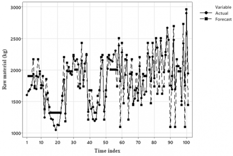
Table 4 shows the forecasting process, including the actual values, initial forecast values, adjustment values, and the final forecast results for each time period. The adjustment values represent corrections applied to improve the accuracy of the initial forecasts. Figure 5 below illustrates the comparison between the actual values and the final forecast values.
Figure 5. Comparison between actual and forecast values using the FTS-MC model
Figure 5 presents the comparison between the actual and forecast values generated by the FTS-MC model. The model evaluation results show a MAPE of 10.91% and an RMSE of 246.94, indicating a relatively high forecasting accuracy. Compared to the ARIMA(2,1,0) model, which achieved a MAPE of 13.67%, the FTS-MC model yielded lower forecasting errors, with a MAPE of 10.91% and an RMSE of 246.94, thereby confirming its superior performance. This advantage arises from the ability of FTS-MC to capture non-linear dynamics and manage uncertainty in fisheries data, which are often affected by environmental variability, seasonal fluctuations, and market-driven shocks. Unlike ARIMA, which is constrained by linearity and stationarity assumptions, FTS-MC incorporates fuzzy logic and probabilistic state transitions, enabling it to more effectively represent irregularities and abrupt changes in the series. Consequently, the FTS-MC model can be regarded as the most appropriate approach for forecasting buffer stock requirements in this context. Based on the forecasting results, the estimated buffer stock requirement for the next period using FTS-MC is 1,975 kg.
This study demonstrates that the ARIMA(2,1,0) model achieved acceptable forecasting performance with a MAPE of 13.67%. Nevertheless, the FTS-MC model produced superior outcomes, with lower forecasting errors (MAPE 10.91% and RMSE 246.94), thereby confirming its greater capability in capturing variability and uncertainty in fisheries data. These findings highlight the critical role of advanced forecasting approaches in supporting sustainable fisheries management, stabilizing supply chains, and improving evidence-based decision-making.
In addition, the conclusion provides practical recommendations for fisheries managers and policymakers. Specifically, fisheries managers are encouraged to implement adaptive buffer stock planning to anticipate seasonal supply shortages, while policymakers can use the forecasting results to improve market stability and protect small-scale fishers from income volatility. These strategies will help strengthen resilience and ensure the long-term sustainability of the fisheries supply chain.
Future research should build upon this work by incorporating broader datasets, real-time monitoring, and environmental variables to further enhance predictive precision across diverse fisheries contexts.
This work is supported by the Ministry of Higher Education, Science and Technology of the Republic of Indonesia.
[1] Naim, S. (2023). Impact of export-import policy changes on the local shrimp fishing industry: A case study of shrimp trade deregulation in Indonesia. West Science Business and Management, 1(4): 296-303.
[2] Vinata, R.T., Kumala, M.T. (2023). Joint security efforts to combat IUU fishing in the waters of Indonesia. Lex Portus, 9(3): 36-49. https://doi.org/10.26886/2524-101X.9.3.2023.3
[3] Misbach, A., Widodo, P., Saragih, H.J.R. (2022). The role of Indonesia customs in the eradication of IUU fishing. Customs Research and Applications Journal, 3(2): 35-54. https://doi.org/10.31092/craj.v3i2.112
[4] Dwi, E.D.S., Hollanda, A.K. (2023). An overview of the Indonesian abalone industry: Production, market, challenges, and opportunities. In BIO Web of Conferences, Bintan Island, Indonesia, p. 02003. https://doi.org/10.1051/bioconf/20237002003
[5] Alcuitas, A.B., Petralba, J. (2023). The sectoral impact of the rice tariffication law on filipino rice supply: A time-series analysis. Recoletos Multidisciplinary Research Journal, 11(2): 85-95. https://doi.org/10.32871/rmrj2311.02.08
[6] Khokhar, M., Zia, S., Khan, S.A., Saleem, S.T., Siddiqui, A.A., Abbas, M. (2023). Decision support system for safety stock and safety time buffers in Multi-Item Single-Stage industrial supply chains. International Journal of Information Systems and Social Change (IJISSC), 14(1): 1-13. https://doi.org/10.4018/IJISSC.324933
[7] Abokyi, E., Strijker, D., Asiedu, K.F., Daams, M.N. (2022). Buffer stock operations and well-being: The case of smallholder farmers in Ghana. Journal of Happiness Studies, 23(1): 125-148. https://doi.org/10.1007/s10902-021-00391-4
[8] Leki, R., Yonathan, B., Kadir, A. (2024). Comparative analysis of volatility levels of 10 stock indices on the indonesian stock exchange on 2 economic events using time series econometric methods. International Journal of Current Science Research and Review, 7(1): 57-65. https://doi.org/10.47191/ijcsrr/V7-i1-06
[9] Ward, E.J., Hunsicker, M.E., Marshall, K.N., Oken, K.L., et al. (2024). Leveraging ecological indicators to improve short term forecasts of fish recruitment. Fish and Fisheries, 25(6): 895-909. https://doi.org/10.1111/faf.12850
[10] Porreca, Z. (2020). Incorporating sea surface temperature into bioeconomic fishery models: An examination of western and central pacific tuna fisheries. https://doi.org/10.20944/preprints202011.0014.v1
[11] Baltazar-Soares, M., Lima, A.R., Silva, G., Gaget, E. (2023). Towards a unified eco-evolutionary framework for fisheries management: Coupling advances in next-generation sequencing with species distribution modelling. Frontiers in Marine Science, 9: 1014361. https://doi.org/10.3389/fmars.2022.1014361
[12] Moustahfid, H., Hendrickson, L.C., Arkhipkin, A., Pierce, G.J., et al. (2021). Ecological-fishery forecasting of squid stock dynamics under climate variability and change: Review, challenges, and recommendations. Reviews in Fisheries Science & Aquaculture, 29(4): 682-705. https://doi.org/10.1080/23308249.2020.1864720
[13] Bolin, J.A., Schoeman, D.S., Evans, K.J., Cummins, S.F., Scales, K.L. (2021). Achieving sustainable and climate-resilient fisheries requires marine ecosystem forecasts to include fish condition. Fish and Fisheries, 22(5): 1067-1084. https://doi.org/10.1111/faf.12569
[14] Zohrah, B.S.P., Bahri, S., Baskara, Z.W. (2024). Forecasting non-metal and rock mineral (MBLB) tax revenue using the fuzzy time series markov chain method in east lombok regency. Eigen Mathematics Journal, 7(1): 8-15. https://doi.org/10.29303/emj.v7i1.171
[15] Pratiwi, S.A., Rachmatin, D., Marwati, R. (2022). Distribution based fuzzy time series markov chain models for forecasting inflation in bandung. KUBIK: Jurnal Publikasi Ilmiah Matematika, 7(1): 11-18. https://doi.org/10.15575/kubik.v7i1.18156
[16] Rusdiana, S., Febriana, D., Maulidi, I., Apriliani, V. (2023). Comparison of weighted markov chain and fuzzy time series-markov chain methods in air temperature prediction in Banda Aceh City. BAREKENG: Jurnal Ilmu Matematika dan Terapan, 17(3): 1301-1312. https://doi.org/10.30598/barekengvol17iss3pp1301-1312
[17] Awan, M.J., Awan, M.M.A., Khan, A.U., Umer, M., Zia, M., Bux, M. (2023). Frequency limited impulse response gramians based model reduction. Mehran University Research Journal of Engineering & Technology, 42(2): 71-74. https://doi.org/10.22581/muet1982.2302.08
[18] Mahmoud Samy Abo El Nasr, M. (2023). Fuzzy time series forecasting: Chen, fuzzy time series forecasting: Chen, markov chain and cheng models. Journal of Alexandria University for Administrative Sciences©, 60(2): 33-45. https://doi.org/10.21608/acj.2023.294123
[19] Makwinja, R., Mengistou, S., Kaunda, E., Alemiew, T., Phiri, T.B., Kosamu, I.B.M., Kaonga, C.C. (2021). Modeling of Lake Malombe annual fish landings and catch per unit effort (CPUE). Forecasting, 3(1): 39-55. https://doi.org/10.3390/forecast3010004
[20] Duan, S. (2023). MOUTAI stock price prediction based on ARIMA model. Advances in Economics, Management and Political Sciences, 14: 34-41. https://doi.org/10.54254/2754-1169/14/20230779
[21] Holmes, E.E., Smitha, B.R., Nimit, K., Maity, S., Checkley, D.M., Wells, M.L., Trainer, V.L. (2021). Improving landings forecasts using environmental covariates: A case study on the Indian oil sardine (Sardinella longiceps). Fisheries Oceanography, 30(6): 623-642. https://doi.org/10.1111/fog.12541
[22] Eighani, M., Cope, J.M., Raoufi, P., Naderi, R.A., Bach, P. (2021). Understanding fishery interactions and stock trajectory of yellowfin tuna exploited by Iranian fisheries in the Sea of Oman. ICES Journal of Marine Science, 78(7): 2420-2431. https://doi.org/10.1093/icesjms/fsab114
[23] Pinnegar, J.K., Hamon, K.G., Kreiss, C.M., Tabeau, A., Rybicki, S., Papathanasopoulou, E., Engelhard, G.H., Eddy, T.D., Peck, M.A. (2021). Future socio-political scenarios for aquatic resources in Europe: A common framework based on shared-socioeconomic-pathways (SSPs). Frontiers in Marine Science, 7: 568219. https://doi.org/10.3389/fmars.2020.568219
[24] Ismail, I., Failler, P., March, A., Thorpe, A. (2022). A system dynamics approach for improved management of the Indian mackerel fishery in peninsular Malaysia. Sustainability (Switzerland), 14(21): 14190. https://doi.org/10.3390/su142114190
[25] Cutler, M.J., Jalbert, K., Ball, K., Bruhis, N., Guetschow, T. (2022). Fisheries co-management in a digital age? An investigation of social media communications on the development of electronic monitoring for the Northeast U.S. groundfish fishery. Ecology and Society, 27(3): 13. https://doi.org/10.5751/ES-13474-270313
[26] Hassouna, F.M.A., Al-Sahili, K. (2020). Practical minimum sample size for road crash time-series prediction models. Advances in Civil Engineering, 2020(1): 6672612. https://doi.org/10.1155/2020/6672612
[27] Talukdar, D., Tripathi, V. (2021). COVID-19 forecast for 13 Caribbean countries using ARIMA modeling for confirmed, death, and recovered cases. F1000Research, 10: 1068. https://doi.org/10.12688/f1000research.73746.1
[28] Akenbor, A.S., Nwandu, P.I. (2021). Forecasting cotton lint exports in Nigeria using the autoregressive integrated moving average model. Journal of Agriculture and Food Sciences, 19(1): 150-162. https://doi.org/10.4314/jafs.v19i1.11
[29] Romanuke, V. (2022). ARIMA model optimal selection for time series forecasting. Maritime Technical Journal, 224(1): 28-40. https://doi.org/10.2478/sjpna-2022-0003
[30] Guo, Z. (2024). Utilizations of the ARIMA model: Empirical findings from the Nasdaq Index. Advances in Economics, Management and Political Sciences, 87(1): 133-139. https://doi.org/10.54254/2754-1169/87/20240892
[31] Lah, M.S.C., Arbaiy, N., Lin, P.C. (2022). An improved ARIMA fitting procedure. In AIP Conference Proceedings, Kuala Lumpur, Malaysia, p. 040005. https://doi.org/10.1063/5.0104053
[32] Wang, P., Huang, W., Zou, H., Lou, X., Ren, H., Yu, S., Guo, J., Zhou, L., Lai, Z., Zhang, D., Xuan, Z., Cao, Y. (2024). Model prediction of radioactivity levels in the environment and food around the world’s first AP 1000 nuclear power unit. Frontiers in Public Health, 12: 1400680. https://doi.org/10.3389/fpubh.2024.1400680
[33] Nath, B., Bhattacharya, D. (2023). Historical pattern of rice productivity in India. Environment Conservation Journal, 24(1): 225-231. https://doi.org/10.36953/ECJ.12292333
[34] Putri, D.M., Afrimayani, Hasibuan, L.H., Ul Hasanah, F.R., Jannah, M. (2024). Comparison of double exponential smoothing and fuzzy time series markov chain in forecasting foreign tourist arrivals. Barekeng, 18(3): 1817-1828. https://doi.org/10.30598/barekengvol18iss3pp1817-1828
[35] Safitri, Y.R. (2022). Comparison of fuzzy time series markov chain and average based fuzzy time series markov chain in forecasting composite stock price index. Jurnal Riset dan Aplikasi Matematika (JRAM), 6(2): 193-203. https://doi.org/10.26740/jram.v6n2.p193-203
[36] Albiento, A.Q., Nopia, J.Z.L., Umpacan, M.C., Mabborang, R.C., Molina, M.G. (2023). Forecasting peak electricity consumption demand in luzon by utilizing ARIMA model. European Journal of Computer Science and Information Technology, 11(2): 37-69. https://doi.org/10.37745/ejcsit.2013/vol11n23769