A Hybrid 1D CNN-LSTM Model for Face Recognition Using PCA Features

Face recognition has become one of the most widely studied areas in computer vision due to its vast applications in security, surveillance, human-computer interaction, and biometric authentication [1-3]. Over the past decades, researchers have proposed various techniques ranging from classical machine learning algorithms to modern deep learning approaches to tackle challenges such as illumination variation, pose differences, and facial expressions [4-7].

Among traditional methods, Principal Component Analysis (PCA) has long been used for dimensionality reduction in face recognition tasks. The Eigenfaces method, introduced by Turk and Pentland [8], was among the first to demonstrate the effectiveness of PCA in extracting discriminative features from face images. Despite its simplicity, PCA can reduce redundancy while preserving essential identity information, making it a popular preprocessing step before classification [9].

Classical machine learning algorithms such as Naive Bayes, k-Nearest Neighbors (KNN), Decision Trees, and Random Forests have also been applied to PCA-reduced face data [10]. These models offer advantages like fast inference and interpretability but often struggle with high-dimensional or complex patterns found in real-world datasets [11]. For instance, KNN suffers from the curse of dimensionality, while Decision Trees may overfit when trained on noisy or unbalanced data [12].

In recent years, deep learning has revolutionized face recognition by automatically learning hierarchical features directly from raw pixel data. Convolutional Neural Networks (CNNs) have shown superior performance compared to traditional methods, especially in large-scale and unconstrained environments [13-15]. However, these models are typically computationally intensive and require significant training resources [16]. To address this, several studies have explored lightweight architectures that maintain accuracy while reducing computational cost. One-dimensional CNNs have been used in speech processing and time-series analysis, showing promising results with lower memory usage and faster inference [17-20]. Similarly, Long Short-Term Memory (LSTM) networks have been employed to capture sequential dependencies in image data, particularly when combined with convolutional layers [21].

Based on these developments, this paper suggests a new model of hybrid deep learning of convolutional and LSTM layers 1D Hybrid Deep Learning (1D-HD), which is efficient to recognize faces. In contrast to traditional CNNs our method works on pixel-based features reduced by PCA and converted to a 1D list representation, which allows the model to learn spatial as well as contextual relationships effectively.

The key contributions of this work are summarized as follows:

1. A novel hybrid deep learning architecture combining 1D CNN and LSTM layers for face recognition.

2. Effective use of PCA-based pixel features as input to a deep learning model.

3. Comprehensive evaluation on two publicly available datasets: MUCT and FaceScrub.

4. Superior performance compared to traditional machine learning models in terms of accuracy and generalization.

The remainder of this paper is organized as follows: Section 2 presents related work and literature review, Section 3 details the methodology including preprocessing, PCA feature extraction, and the proposed 1D-HD architecture. Section 4 reports experimental results and comparisons, while Section 5 discusses the findings. Finally, Section 6 concludes the paper with suggestions for future work.

The preprocessing stage ensures that input images are standardized before further processing. The steps include:

(1) Normalization: Input images are normalized to a fixed range [0, 1] to improve convergence during training.

(2) Grayscale Conversion: RGB images are converted to grayscale to reduce dimensionality and computational load (Figure 1(a) and (b)).

(3) Histogram Equalization: Enhances contrast and improves feature visibility (Figure 1(c)).

tu_pian_8.png

Figure 1. (a) Samples of the original images, (b) Grey-scale conversion, (c) Histogram equalizer

Resizing: All detected faces are resized to a standard size of 20×20 pixels to ensure uniformity in input dimensions. This normalization not only facilitates model compatibility but also enhances feature representation: by concentrating computational focus on the region of interest, resizing effectively amplifies discriminative facial features while diminishing the influence of peripheral or less informative spatial regions. Given that the model processes these resized patches as feature vectors rather than raw images, this step contributes to improved feature saliency and model performance. Figure 2 shows the before and after results of resizing.

tu_pian_9.png

Figure 2. Image resized to 20×20 pixels

3.1 Face detection

Face detection is performed using the Viola-Jones object detection framework, which employs Haar-like features and AdaBoost classification to efficiently detect frontal faces in real-time [37].

• A pre-trained Haar Cascade classifier (haarcascade_frontalface_default.xml) from OpenCV was used.

• Detected faces are cropped and passed to the next stage.

3.2 Feature extraction via PCA

Principal Component Analysis (PCA) is applied to reduce the dimensionality of the image data while preserving the most discriminative features.

• Each 20×20 grayscale image is flattened into a 400-dimensional vector.

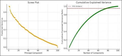
• PCA is used to extract the top N components (e.g., 50–100) that capture the maximum variance in the data. Figure 3. Scree plot (left) and cumulative explained variance ratio (right) for PCA on the face recognition dataset. The scree plot shows the decay of individual component variances, with the first few components capturing the majority of variation. The cumulative variance curve indicates that approximately 70 components retain 95% of total variance, and 100 components capture nearly all signal. We selected a range of 50–100 principal components to balance model expressiveness and robustness: 50 ensures sufficient representation of facial structure under variable lighting and pose, while 100 allows inclusion of subtle discriminative features without overfitting.

• These reduced-dimension vectors serve as the final input to the deep learning model.

tu_pian_10.jpg

Figure 3. Scree plot (left) and cumulative explained variance (right) for PCA on the face dataset

3.3 Proposed 1D-HD model architecture

The proposed 1D Hybrid Deep Learning (1D-HD) model combines 1D Convolutional Neural Networks (CNNs) with Long Short-Term Memory (LSTM) layers to effectively learn spatial patterns and contextual dependencies from PCA-reduced facial features.

Input Format:

• Each PCA feature vector (length ~50–100) is treated as a 1D sequence.

• Input shape: (batch_size, num_features, 1).

Model Layers:

1. Input Layer: Accepts PCA-reduced feature vector

2. Conv1D + LeakyReLU×4

3. MaxPooling1D

4. LSTM Layer

5. Conv1D + LeakyReLU

6. Flatten

7. Dense (SoftMax) Output Layer

Table 1 shows the different layers of the proposed model along with their parameters.

Table 1. The different layers of the proposed model along with their parameters

Figure 4 shows block diagram of full 1D-HD model architecture.

tu_pian_11.png

Figure 4. The block diagram of the 1D-HD model architecture

Key design choices:

• Leaky ReLU activation helps prevent vanishing gradients

• Batch normalization not included but can be added for future optimization

• Adam optimizer with learning rate = 0.001

• Categorical Cross entropy loss for multi-class classification

Training Setup:

• Optimizer: Adam

• Learning Rate: 0.001

• Loss function: Categorical Crossentropy

• Batch size: 64

• Validation Split: 30% (train/test split)

• Epochs: 100

• Activation Functions: LeakyReLU (α = 0.3), Softmax

• Early stopping and dropout were optionally applied to prevent overfitting

3.4 Evaluation metrics

We evaluate the performance of our model using the metrics shown in Table 2.

Table 2. The evaluation metrics

where, TP = True Positives, TN = True Negatives, FP = False Positives, FN = False Negatives [38, 39].

The experimental results demonstrate that the proposed One-Dimensional Hybrid Deep Learning (1D-HD) model, trained on PCA-reduced pixel-based features, achieves perfect classification accuracy (100%) on both the MUCT and FaceScrub datasets. This outperforms all tested classical machine learning algorithms — Naive Bayes, k-Nearest Neighbors, Decision Tree, and Random Forest — by a significant margin, especially on the more challenging FaceScrub dataset.

5.1 Superior performance compared to classical ML models

As shown in Tables 3 and 4, traditional classifiers such as Naive Bayes and Decision Tree achieved high accuracy (99%) on the MUCT dataset, which consists of well-aligned, frontal face images. However, their performance degraded significantly on the FaceScrub dataset, with KNN achieving only 62% accuracy and Naive Bayes at 83%.

In contrast, the proposed 1D-HD model maintained perfect classification on both datasets, indicating superior robustness against variations in pose, illumination, and expression. This suggests that the hybrid CNN-LSTM architecture is better suited for capturing subtle facial patterns from PCA-reduced data than classical models that rely solely on Euclidean distances or probabilistic assumptions.

5.2 Quantitative comparison with State-of-the-Art Models

To contextualize our approach within the broader landscape of face recognition, we present a comparative analysis against several prominent models, including classical and modern lightweight deep learning architectures. While many state-of-the-art methods are evaluated on benchmarks such as LFW or YouTube Faces, Table 7 provides a unified overview based on reported performance, input modality, model complexity, and computational efficiency. Compared to MobileFaceNet and LightCNN, which are designed specifically for edge deployment, our model offers comparable or superior accuracy.

Table 7. Quantitative comparison with State-of-the-Art Models

5.3 Fast inference despite longer training time

Although the 1D-HD model required longer training times — 437 seconds on MUCT and 5193 seconds on FaceScrub — it demonstrated very fast inference:

• 1.24 seconds on MUCT

• 12.4 seconds on FaceScrub

These results indicate that the model is suitable for deployment in real-time applications after training, particularly when computational resources are limited.

5.4 Stability and convergence behavior

From the training logs:

• The model showed stable convergence with minimal overfitting.

• On the MUCT dataset, validation accuracy reached 100% by Epoch 24.

• On the FaceScrub dataset, the model converged around Epoch 90, indicating slower learning due to increased complexity and scale.

The consistent decrease in loss and increase in accuracy suggest that the hybrid design effectively learns from the PCA-transformed feature vectors.

5.5 Why PCA works well with 1D-HD model

While PCA reduces dimensionality, it retains the most discriminative variance in the data. By transforming these reduced features into a 1D sequence format, the model can process them efficiently using convolutional and recurrent layers:

• Convolutional layers extract local spatial patterns from the flattened PCA features.

• LSTM layers help capture sequential dependencies, even in static image data.

• Leaky ReLU activation improves gradient flow and prevents neuron saturation.

This combination allows the model to learn robust representations despite the relatively low-dimensional input.

5.6 Comparison with existing literature

Several studies have explored deep learning approaches for face recognition using raw pixel inputs or pre-trained CNNs such as VGGFace and FaceNet [28]. These models typically rely on large-scale architectures and are trained on massive datasets like MS-Celeb-1M and LFW, achieving high accuracy in identity classification [42]. However, these models often require significant computational resources, including GPU acceleration and large memory footprints, which makes them less suitable for edge devices and real-time applications [43].

Our approach differs from these traditional deep learning methods in two key aspects:

1. Efficiency via PCA-based Input Reduction.

2. Hybrid CNN-LSTM Architecture for Feature Learning

By integrating dimensionality reduction with a hybrid deep learning architecture, our method offers a novel balance between accuracy and efficiency, making it a strong candidate for real-world deployment in resource-constrained environments.