Tariq A. Hassan*![]() | Hesham A. Alabbasi
| Hesham A. Alabbasi![]() | Rehab I. Ajel
| Rehab I. Ajel![]()
© 2025 The authors. This article is published by IIETA and is licensed under the CC BY 4.0 license (http://creativecommons.org/licenses/by/4.0/).
OPEN ACCESS
This paper presents a source–filter compressive sensing (CS) technique for speech signal compression. The model adopts sparse representation methods to estimate both source and frequency envelop or filter components of speech. Traditional approaches such as Linear Predictive Coding (LPC), Mel-Frequency Cepstral Coefficients (MFCC), and Perceptual Linear Prediction (PLP) typically produce dense parameter vectors, which are not inherently sparse. In contrast, the method introduced here leverages CS and sparse coding to represent the source and filter parameters in a sparse format Two objectives are addressed: (i) estimating predictive coefficients in a sparse mode, and (ii) employing a data-driven dictionary or sensing matrix, generated directly from the speech signal, as an alternative to generic bases such as the Discrete Cosine Transform (DCT) or Fast Fourier Transform (FFT). The implementation of the framework is done with the most widely used software languages Python and MATLAB. The performance of the proposed technique is evaluated against LPC-based parameter estimation and DCT-basis CS. Experiments are conducted on both voiced and unvoiced speech signals. Results show that the data-driven source–filter dictionary improves reconstruction quality compared to conventional DCT-based CS. Sparse estimation is carried out using CVX and Least Absolute Shrinkage and Selection Operator (LASSO), and their outcomes are compared. System performance is assessed using quantitative metrics such as Mean Square Error (MSE) and Signal-to-Noise Ratio (SNR), showing consistent improvements in speech compression and reconstruction accuracy.
speech compression, sparse representation, source-filter model, compressions software, compressive sensing, data-driven dictionary, LPC, CVX, LASSO
Since the beginning of humankind, speech has been the main means of human-to-human interaction. With the development of life towards digital communication, signals have become increasingly complicated in terms of processing, storage, or even transmission. As a result, data becomes huge and hard to manage. Therefore, in recent years, many techniques and software have been proposed and to reduce the data size by either removing some unnecessary components (i.e., lossy compression) or lowering the bit rate or sample rate to a level that does not affect the speech signal (lossless compression) [1, 2].
Techniques like Wavelet transform [3], Huffman Coding [4], Lempel-Ziv-Welch (LZW) [5], Adaptive arithmetic Coding [6], Discrete cosine transform [7, 8], linear predictive coding (LPC) [9], and other techniques which are implemented in various software languages that are utilized in signal compression with different levels of compression ratio, complexity, information lost, and the clarity of signal reconstruction.
In recent years, technique called compressed sensing (CS), a method exploits the sparsity of nearly all signals in nature [10]. Signals like speech, show their sparse nature especially with short period of time [11]. Thus, segmenting the signal before processing will be an essential step for proper compression.
Nyquist’s theorem, that the CS technique try to defeat, state that for any digital signal the sampling rate needed to be equal to or greater than twice the highest frequency of the signal [12].
In contrast, the CS technique suggests that a signal can be represented or reconstructed from a smaller number of components or samples as its shows a level of sparsity in one domain, much fewer than the Nyquist sampling rate. Beating the Nyquist restriction is the key role of the CS model in terms of signal encoding and compression.
Accordingly, CS has found interest in many applications, such as signal processing, medical imaging, wireless communications, image and video processing, audio and acoustics, and remote sensing. In the study [13], the compressed sensing technique, along with Long Short-Term Memory (LSTM) networks used for speech reconstruction enhancement in a noisy environment. The model suggests that the CS can enhance the system performance in terms of time complexity and prior knowledge of the signal.
The technique proposed in the reference [14] adopted sparse Bayesian inference (SBI) and nonnegative matrix factorization (NMF) in two separate speech signals. It states that the spatial information can be better estimated with SBI compared with traditional compressed sensing. Also, CS can be used in reconstructing the signal generated from the neural network by sparse latent inputs [15]. The authors in the reference [16] presented some main applications that used the CS in their proposed systems, such as Radar, sonar, video and audio processing, and other applications that find the CS is a very effective technique in terms of time consumption and signal size.
Some papers [17, 18] used what it called data-driven sensing matrix or dictionary to estimate some features presented in signal data or to extract the signal or image buried under noisy data.
In this paper, a model takes advantage from a compressed sensing perspective and sparse optimization is presented for speech signal compression. The proposed system will utilize the combination of the LPC method and sparse coding.
The proposed model will deal with the speech signal as two parts, namely, the frequency envelope coefficients, which represent frequency resonance of the vocal tract (VT). The second part is the source signal (residual), which will be either a train of pulses (in the case of voiced speech) or a noise-like signal (in the case of unvoiced speech). The vocal tract envelope and its excitation signal (source) with converted to sparse vectors holding only effective parameters without reducing the signal clarity. In other words, need to compress both parts of the speech signal (i.e., the source excitation signal and filter or envelope) to the level that the system can reconstruct the original signal (as close as possible to the original signal) without distorting or deforming the original speech. The main challenge in this system is how to create or derive a data-driven dictionary matrix, which is used to represent the signal in compact form (create a vector of fewer measurement that represent the original form). The idea is how to choose the proper dictionary matrix (DM) that would be convenient with the speech data and it will be the key role of the highest sparsity and best compression ratio alike. In the sparse coding and compressed sensing-based methods, there have been many suggested dictionary matrices, such as DCT, FFT, and DWT matrices. As the signal and the system performance are highly sensitive to the selected dictionary matrix, which consequently affects the algorithms used to recover the original signal. The contribution in this paper is to suggest that the DM will be created from the signal itself, a step that plays a huge role in system performance. The effective columns of DM, called atoms, later will be the seed for speech signal reconstruction.
As mentioned earlier, Compressive Sensing (CS) is an effective way in signal processing methodology that enables reliable reconstruction of sparse signals from a reduced number of observations or measurements, far below the Nyquist sampling rate. These sparse signals will hold the most effective components of the signal that will be used to store, transmit, or reconstruct the original signal. In other words, once the signal is compressed, there is no need to store or transmit the whole signal; just a few non-zero values (sparse vector) will be enough to rebuild the speech signal.
Finding the sparse vector that is compatible with the signal measurements is not an easy task and needs a special kind of algorithms that promote sparsity (these algorithms are normally called convex algorithms used to find the sparse solution by L1_norm). These methods like; Basis pursuit (BP), Least Absolute Shrinkage and Selection Operator (LASSO), Orthogonal Matching Pursuit (OMP) and so many other methods are used to enforce sparsity in the solution vector and solve an underdetermined system (systems when the variables are more than the equations) [19]. An alternative to these approaches is the greedy algorithms (such as CVX and CoSaMP), which are easy and computationally efficient and use an iterative matching Pursuit for the L1_minimization problem.
These algorithms estimate the original signal using a linear combination of fewer components of a learned dictionary (some vector of an over-complete dictionary called atoms) with a (K-sparse) signal or sparse code (a signal that has only K non-zero values). The algorithms do not emphasize that the atom vectors have to be orthogonal, which makes them flexible to adapt to the specific speech signal.
Mathematically, if $f \in \mathrm{R}^{\mathrm{n}}$ is a compressible signal in some domain, say frequency domain for example, then it is possible to select a set of components (far fewer samples or measurements called sparse measurements) to represent the original signal without losing the important details [20].
$f=\Psi s$ (1)
where, $s$ is The coefficient vector contains entries that are almost zeros or near zero, $\Psi \in \mathrm{R}^{\mathrm{n} \times \mathrm{n}}$ is the transform basis matrix, or sparse basis (such as FFT, DWT, or DCT).
In this case, $s$ will contain only K non-zero values (the signal will be called K -sparse signal), where K is far less than the actual length of the signal.
For example, the $\Psi$ matrix is the wavelet basis, $\Psi=\left[\Psi_1 \Psi_2\right. \left.\psi_3 \ldots \psi_n\right]$, then the original signal $f$ can be represented as:
$f(t)=\sum_{i=0}^n s_i \psi_i(t)$ (2)
In this context, the signal $f$ is expressed as a weighted combination of the coefficient vector and the basis functions.
Let's say it in another way: if $f$ is a signal in the time domain (such as a speech signal), then there is another representation of the signal in another domain (the frequency domain) that describes the actual signal $f$ with many fewer components. In Eq. (1), $f$ and $s$ are both of the same length ($f, s \in \mathrm{R}^{\mathrm{n}}$), but the vector $s$ contains only K non-zero values, and the others are either zeros or nearly zero values.
In this case, the original signal f can be reconstructed using a few terms of the linear combination between the basis matrix Ψ and the sparse signal vector s. The only constraint is that the transform basis must be generic. In short, a generic transform basis should have two properties: first, incoherence (low correlation with the sparsifying basis); second, the Restricted Isometry Property (RIP), which preserves the distances between sparse vectors when projected [21].
In compressive sensing theory, an essential term that plays a vital role, especially in signal acquisition or representation that is the measurement matrix.
The measurement matrix is the mathematical operator that transform the high-dimensional signal $f \in \mathrm{R}^{\mathrm{n}}$ into a lowerdimensional collections of measurements $y \in R^m$ where $m \ll n$ :
$y=\varphi f$ (3)
where, y is a vector holding values of random positions of the original signal, $\varphi \in R^{m \times n}$ is the measurement matrix [20].
In this formula, we project (correlate) each row of the measurement matrix (sensing function) with the signal samples to generate a single measurement represent one component. The vector components in y later be used to reconstruct (estimate) the original signal f.
The measurement matrix is theoretically chosen to satisfy the criteria of incoherence and/or the limited isometry property, hence ensuring the reliable reconstruction of sparse signals.
To make things clear, in order to recover $f$ in classical signal processing, we require at least as many measurements as the signal dimension $(m \geq n)$. Sensing functions (the rows of the measurement matrix) $m$ must, however, be significantly smaller than the signal's dimension $n$ in order to use the compressed sensing technique. Reconstruction or recovery can be accomplished with just these few observations if the signal has sparse characteristics in some domain. Therefore, when we enter formula (1) into the linear model (3), we obtain:
$y=\varphi f=\varphi \Psi s$
Define $A=\varphi \Psi$, so
$y=A s$ (4)
where, $A \in \mathrm{R}^{\mathrm{m} \times \mathrm{n}}$ is the dictionary matrix, set of basis vectors used to sparsify the signal. This formula states that the compreed version of the signal $y$ can be expressed as a linear combination of sparse vector $s$ with only a few dictionary columns (atoms).
The compressed sensing algorithms will be used to find the sparse vector $s$ under this constraint [20];
$\hat{s}=\underset{s}{\operatorname{argmin}}\|s\|_1$ subject to $y=A s$ (5)
where $\|.\|_1$ is $L_1$ norm and $\hat{s}$ is the estimated sparse signal. Estimating $s$ will then used to recover the signal $f$ using (1). Adoping 1_norm minimization is for two reasons; first, it will ensure that the solution is sparse (which is opposite to the $L_2$ norm, which will not guarantee a sparse solution. Second is convex, namely, the solution can be found with less computational complexity. Moreover, the selection of the dictionary matrix $A$ is very crucial in compressed sensing it could skew the signal values to the level that will be unable to reconstruct the original signal [21]. One of the fundamental concepts of dictionary learning is that the dictionary must be derived from the incoming data. The fact is that the sparse technique needs to use a minimal number of dictionary components in order to represent the original signal. Previously, predetermined dictionaries such as Fourier or wavelet transformations were commonly used. In some circumstances, a dictionary gained from the original input data can considerably enhance the sparsity.
In this section, the main steps of our proposed system will be presented. The system is composed of phases. The first phase will involve signal separation into two parts: the signal source (of the excitation signal or residual of the LPC method), and the filter (the frequency envelope or vocal tract filter). These two parts of the signal will pass into the second phase, which will involve estimating the sparse version (the compressed mode of the signal parts). The two phases, along with their main steps and equations, will be illustrated in the next subsections.
3.1 Excitation and frequency envelop components of the speech signal
Basically, one of the most practical representations of the speech signal is to present it as two crucial interacting components (ingredients) that convolve in time domain to produce a specific word sound. These are: the excitation signal produced either at vocal folds (in the case of voiced speech) or a noise-like signal produced at the vocal cavity (in the case of unvoiced speech). In both cases, the excitation signal will be shaped by the vocal tract organ (which will work as a set of band-pass filters around the resonance frequencies). Many methods are utilized to estimate (or extract) these components from speech. Methods like MFCC, PLP, LPC can estimate the vocal tract envelope coefficients and use them as filter parameters to extract the residual signal (the source signal).
LPC technique is one of the best methods used in speech compression [22]. This approach states that the speech signal can be approximated as a linear combination of the past speech samples with a set of predictive coefficients (a set of parameters estimated by the LPC approach) [22].
$f[i]=\sum_{p=0}^P \alpha_p f[i-p]+e[i], \quad i=1..n$ (6)
where, a is the prediction coefficients or weights, and e is the error or residual signal (excitation signal in the case of voiced signal, or noise-like signal in the case of unvoiced signal). The task is to estimate the prediction coefficients (which represent the formant frequency envelope of vocal tract filter parameters) and the source signal (which represent the excitation of the speech signal). Many methods have been presented to estimate the production coefficients, such as Autocorrelation, Covariance, and Maximum Likelihood Estimation (MLE) methods [23].
As we mentioned above, one of the successful signal recovery methods is the proper selection of the sensing matrix (A in this article).
In the paper, we will take advantage of the original equation of speech (6) to build up the sensing matrix with columns equal to the filter coefficient length p (here p = m in formula (3)), and use it as a dictionary matrix for sparse signal coding. The matrix will build as follows:
$A=f[1 . . n-p, 2 . . n-(p-1) \ldots, p . . n]$ (7)
Here, A will represent the measurement matrix (with rows = p and columns = (n — p). Each row is representing a sensing waveform estimated from the signal itself with one-values shifted of the signal to maintain the matrix width (size) and to cover all signal samples. These sensing waveforms represent the dictionary atoms and it will be used (in our proposed system) as the dictionary or compressive sensing basis for signal compression.
3.2 The sparsity of the excitation and the envelop parameters
The proper dictionary or sensing matrix is the key role in compressed sensing and sparse representation of the signal. In our model, the dictionary matrix is formed from the signal itself. Compressive sensing technique aims to reconstruct the original signal f (or its sparse coefficients s) from the reduced measurements y by solving the optimization problem. In our proposed model, the optimization problem will utilize the frequency envelop coefficients a and the source signal r. The convex optimization is as follow:
$\underset{\alpha, r}{\operatorname{argmin}}\|A \alpha-f\|_1+\beta\|r\|_1+\Lambda\|\alpha\|_1$ (8)
subject to
$A \alpha+r=f$
where A and $\alpha$ are as mentioned before, $r \in \mathrm{R}^{\mathrm{n}}$ in the source signal (residual), $\lambda$ is the regulator parameter (or scale) used to control the level between accuracy and sparsity of the prediction coefficients (or envelop coefficients), $\beta$ is the scale that regulate the sparsity in source signal $r$. The goal of this system equations is to estimate the frequency envelop coefficients vectors $\alpha$ and source signal $r$ in their most sparse representation and using them to reconstruct the original speech signal with tolerated error.
Actually, LPC and inverse filtering techniques can be used to estimate these two vectors, however, the resulting values are not sparse and the reconstructed signal needs full-valued parameters of both vectors.
Many methods are used to solve this optimization. In our proposed system, we used CVX (as a software package within the MATLAB environment) and LASSO methods. In fact, LASSO results were nearly as same as CVX. However, CVX can estimate $\alpha$ and $r$ vectors at the same time, LASSO on the other hand can only be used to estimate frequency envelope coefficients ($\alpha$), then an inverse filter is used then to estimate the sparse source signal ($r$).
Also, the system tested with different values of $\lambda$ and $\beta$ parameters to examine how these parameters can affect the sparsity and the quality of signal reconstruction.
For $\alpha$ parameters, the number of coefficients will be set to be between 20-45 coefficients (by experiment this range is the best for the $\alpha$ parameters).
In terms of the source signal parameters r generated by this model is, most of their values are zeros or nearly zeros. Thus, a threshold is used to regulate the signal sparsity by setting low values (below the threshold) to zero.
In this paper, we proposed a compressive sensing framework for speech signal compression, exploiting the useful diverse function and libraries for signal processing which are provided by Python and MATLAB to write the code of the system [24, 25]. The system utilized the LPC strategy to construct a special measurement or sensing matrix then use it to generate the source signal r and the frequency envelop coefficients a in a sparse mode. These vectors (r and α) are then used to recover the original speech signal.
Here the dataset can be any speech signal. There is no restricted to some kind of data. The only need requirement is the signal has to be clean (unnoisy signal) since no noise removal is used in this system.
This section will present the signal compression results of the sparse optimization of the α and r vectors of the system equation (8). The sparse coding techniques CVX and LASSO will be used in our experiment and the results will compare with technique adopt DCT basis matrix in compressive sensing. The compression ratio and error measurements are used to examine the system performance with different values of sparsity levels.
The system will utilize two types of speech signals: voiced and unvoiced. First, the speech signal is divided into fixed-length frames, typically ranging from 20 to 30 milliseconds. This approach is used because speech within this time frame tends to be quasi-stationary, resulting in parameters that show minimal fluctuation.
The optimization algorithms are utilized to find the sparsity values for the envelope parameters and the source signal (α and r). By the experiment, both algorithms (CVX, LASSO) will generate a sparse frequency envelope coefficients α and sparse source signal r. For the source signal, a threshold parameter will be applied to set coefficients with small values to zero. The result is sparse vectors that represent the source and filter coefficients with fewer values than those produced by LPC method.
In our proposed system, no DCT or FFT transform has been used, so signal analysis will stay in the time domain. The goal of our system is to use the speech data to build up the measurement matrix, which in turn, will ensure that the L1-Norm optimization will estimate the sparsest solution for the parameters. Basically, this idea benefits from the learning-based approach, which exploits the real data in modeling and processing the signal [26].
Using both terms of the speech signal (source and the predictive coefficients) will reduce the system complexity and reduce calculation time as well as will guaranteed that the produced source signal and prediction coefficients are correlated. In fact, CVX optimization method can estimate both vectors, however, LASSO method need an extra step (inverse filtering) to estimate the source signal.
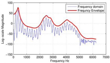
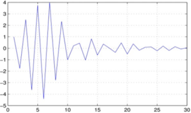
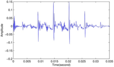
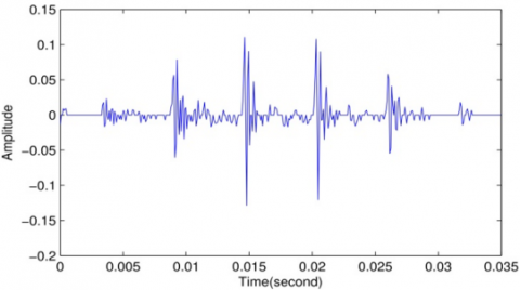
Figure 1. Speech signal spectral and its envelope estimated using LPC method with p=30 (a), predictive coefficients (b), and the source signal (c)
In order to evaluate the proposed system, the test materials are signal frames segmented from a speech signal with a sampling frequency 12500 Hz. Figure 1 gives an example of the spectra and frequency envelope for voiced speech, the predictive coefficients, and the source signal estimated using LPC and inverse filtering respectively.
In the compression scenario, these two vectors (prediction coefficients and the source signal) would not effectively contribute to the data reduction since they both are fully-valued vectors (dense format).
To reconstruct the original signal, these two parts of the speech (the source signal the predictive coefficients) have to recombined together.
An alternative technique is to use the sparse optimization algorithms to estimate these two vectors in sparse, which means that only few parameters (or significant) will need to reconstruct the original signal.
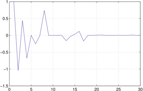
Figure 2 shows the sparse prediction coefficients and the sparse source signal of the same voiced frame. These vectors are about only 40% sparse level (only 40% of its data are non-zero values).
Figure 2. Sparse predictive coefficients (a) and sparse source signal (b)
In our algorithm, first, we need to build up the dictionary matrix out of the data of each frame. It will work like a key mark that characterizes each speech frame (speech segment) to build its own dictionary. Then, use the generated matrix (dictionary) to estimate the predictive coefficients and the source signal in sparse format.
CVX algorithm is used to estimate the source and the envelope coefficients simultaneously. This mean that the envelope coefficients and the source signal will estimate at the same time and there is no need to use the inverse filter to estimate the source signal.
As stated in formula (8) $\beta$ and $\lambda$ parameters use to regulate the sparsity level in source signal and predictive coefficients respectively.
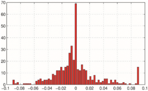
Figure 3 shows the histogram of the source signal with different values of $\beta$. The figure shows the effect of two $\beta$ regulators on the source signals. From the hierograms we can notes that the sparsity will increase by decrease the value of the regulator $\beta$ and vice versa.
Figure 3. The Histogram of the sparse source signal of different values of $\beta$ regulator. $\beta=0.05(\mathrm{a}), \beta=5$
The utility of the proposed system in Eq. (8) with different regulators quantities is evaluated in a voiced and unvoiced speech signal compression task. We compare the performance of our proposed system using CVX and LASSO techniques in estimating the sparse solution of the source and predictive coefficients components with the DCT basis compressive sensing compression of the speech signal.
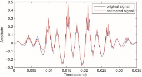
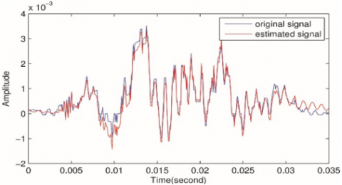
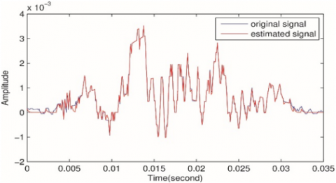
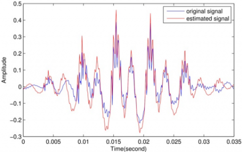
Figures 4(a)-(c) summarize the results of the comparison between the original speech signal with the reconstructed signal of different values of sparsity regulators $\beta \text { and } \lambda$.
Figure 4(a) shows the original and reconstructed voiced speech singles for β=5, ⅄=0.5 with source sparsity level=42% of the original length. The MSE error between the original signal and the reconstructed signal is 2.8817e-04, and SNR=16.8863.
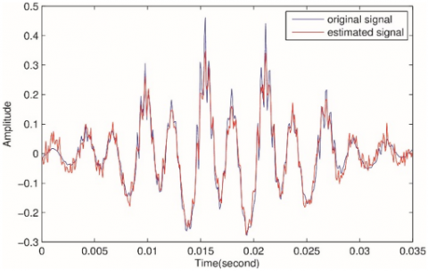
Figure 4(b) shows the signals with β=0.5, ⅄=0.1 and sparsity level=73%. The MSE= 4.9655e-05, and SNR= 24.5231.
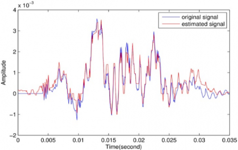
Figure 4(c) summarizes the accuracy of the original and the reconstructed unvoiced speech signal. The regulation parameters are as follow; β=5, ⅄=0.01, the sparsity level= 45%. MES= 4.3556e-08, SNR= 14.0132.
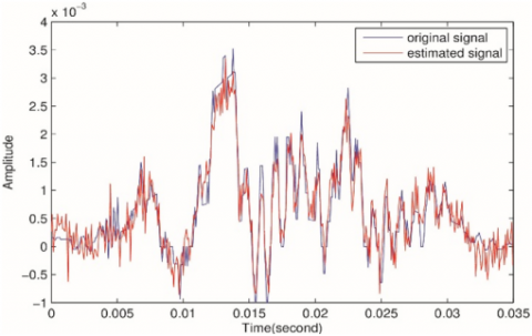
Figure 4(d) shows the accuracy of the signals (unvoiced) with β=2, ⅄=0.5, the sparsity level= 64%. MES= 3.8661e-09, SNR= 24.5310.
Figure 4. The original signal with its reconstructive counterpart of voiced and unvoiced speech
As mentioned before, we can change the sparsity level by changing the values of the regulator parameters $\beta \text {and} \lambda$, however, this can affect the compression ratio, error measurement and the reconstruction accuracy.
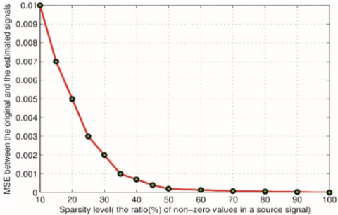
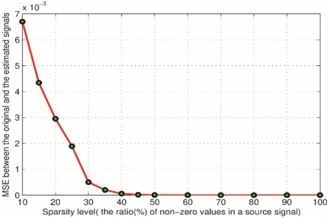
Figure 5. Sparsity level vs. the MSE error measurement between the original and estimated signals, voiced speech (a), unvoiced speech
Figure 5 shows the MSE error between the original and the estimated signals of different levels of source signal sparsity with fixed filter coefficients p = 30. It is clear that the MSE will decrease as the sparsity level increases (increasing the non-zero or significant values). We always need to take care of the sparsity level and compression ratio.
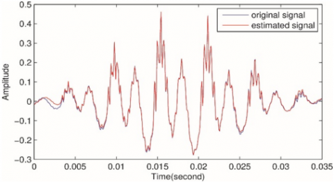
Figure 6. The original and the estimated signal out of sparse source and envelope coefficients using LASSO technique
Other optimization technique like LASSO can also be used to estimate the sparse vectors of the source-filter model, but it needs more than one round for sparse components estimation. The first round will be to estimate the sparse filter or envelope coefficients. Then, the second step, is to use the inverse filter to estimate the source signal. LASSO cannot estimate the two vectors simultaneously as the CVX does. Figure 6 shows the original and the estimated signals using LASSO technique. To examine to what extent the proposed system produces better performance in terms of compression ratio and reconstruction accuracy, Figure 7 illustrates the results of speech signal compression and reconstruction using compressive sensing with DCT basis dictionary.
Figure 7(a) shows the original and reconstructed voiced speech singles with signal sparsity level=45% (y length of system Eq. (2), here p=200 and n=450 (the signal frame length). The MSE error between the original signal and the reconstructed signal is 5.3840e-04, and SNR= 14.1717.
Figure 7(b) summarizes the results of the unvoiced speech, the sparsity level= 45%. MSE= 2.3170e-07, SNR= 10.7110.
Figure 7. Compressive sensing using DCT basis dictionary for voiced speech (a) and unvoiced speech (b)
The experimental results presented in Figures 4 and 6 demonstrate the effectiveness of employing a data-driven dictionary matrix in compressive sensing for speech compression. Compared with the traditional DCT-basis approach (Figure 7), the proposed system invariably achieves lower reconstruction error and higher signal quality. A key factor in this improvement is the use of sparse source signals together with sparse envelope coefficients, which enable more accurate recovery of both excitation and spectral envelope characteristics of speech. By jointly exploiting these sparse representations, the system produces a more faithful reconstruction of both voiced and unvoiced segments. This advantage is reflected in the quantitative measures: The Mean Square Error (MSE) is reduced, while the Signal-To-Noise Ratio (SNR) is improved relative to the DCT-based CS system. These results confirm that adapting the dictionary to the statistical structure of the speech signal-while leveraging sparsity in both source and filter domains-yields more efficient compression and reconstruction, validating the central premise of our approach.
This paper has presented a new encoding technique that rely on the sparse optimization methods. The technique was able to estimate the elements of the two parts that model the speech signal, namely, the source and filter in a sparse form. One of the main challenges in sparsity techniques is the selection of the proper dictionary matrix. In this system, the matrix was built from the signal itself. This makes the system converge easily to the best sparse solution (the sparsest solution). The system is tested with two different types of speech, voiced and unvoiced. Results show that the unvoiced signal can be reconstructed with highly sparse source and filter coefficients. This is because the unvoiced signal holds less energy, especially at the low-frequency part of the signal. Also, the experiment shows that the level of sparsity (the amount of zero values present in the signal) can increase the compression ratio, however, it can affect the reconstruction accuracy since it will ignore a lot of important information presented in the speech signal. So, it is always very important to follow a trade-off between the accuracy and the sparsity level. Finally, there are many methods presented for sparse relaxation (optimization). However, some need more than one round to estimate both signal parts, such as LASSO. Others need more steps to converge, such as OMP. CVX, on the other hand, Python and MATLAB are the best choice in coding the system, it is easy to apply (a MATLAB and Python package is available for free), and it usually converts the problem to standard form and always converges to the sparsest solution. Also, it returns the sparse solution of the source signal and filter (or frequency envelope) coefficients at once.
Conceptualization, 1st and 2nd; methodology, 1st; software, 3rd; validation, 1st, 2nd, and 3rd; formal analysis, 1st; investigation, Rehab; resources, 1st; data curation, 1st; writing—original draft preparation, 3rd; writing—review and editing, 2nd; visualization, 1st; supervision, 2nd; project administration, 2nd; funding acquisition, 3rd.
All authors have read and agreed to the published version of the manuscript. Authorship is limited to those who have contributed substantially to the work reported.
The authors would like to express their thanks and gratitude to Mustansiriyah University, College of Education, and the computer department for their facilities and support in this work.
[1] Kondoz, A.M. (2024). Analysis by Synthesis LPC Coding. In Digital Speech, pp. 199-260. John Wiley Sons, Ltd. https://doi.org/10.1002/0470870109.ch7
[2] Gold, B., Morgan, N., Ellis, D. (2011). Speech Synthesischapter. In Speech and Audio Signal Processing: Processing and Perception of Speech and Music, pp. 431-454. Wiley. https://doi.org/10.1002/9781118142882.ch30
[3] Pal, R. (2021). Speech compression with wavelet transform and huffman coding. In 2021 International Conference on Communication Information and Computing Technology (ICCICT), Mumbai, India, pp. 1-4. https://doi.org/10.1109/ICCICT50803.2021.9510116
[4] Hamza, R.K., Rijab, K.S., Hussien, M.A. (2021). The ECG data compression by discrete wavelet transform and huffman encoding. In 2021 7th International Conference on Contemporary Information Technology and Mathematics (ICCITM), Mosul, Iraq, pp. 75-81. https://doi.org/10.1109/ICCITM53167.2021.9677704
[5] Shrividhiya, G., Srujana, K.S., Kashyap, S.N., Gururaj, C. (2021). Robust data compression algorithm utilizing LZW framework based on huffman technique. In 2021 International Conference on Emerging Smart Computing and Informatics (ESCI), Pune, India, pp. 234-237. https://doi.org/10.1109/ESCI50559.2021.9396785
[6] Sudhamsu, G., Singh, S., Gautam, C.K. (2024). Efficient Lossless data compression using adaptive arithmetic coding. In 2024 15th International Conference on Computing Communication and Networking Technologies (ICCCNT), Kamand, India, pp. 1-6. https://doi.org/10.1109/ICCCNT61001.2024.10725862
[7] Jamal, M., Hassan, T.A. (2022). Speech coding using discrete cosine transform and chaotic map. Ing´enierie des Syst`emes d’Information, 27(4): 673–677. https://doi.org/10.18280/isi.270419
[8] Hassan, T.A., Al-Hashemy, R.H., Ajel, R.I. (2019). Speech signal compression algorithm based on the JPEG technique. Journal of Intelligent Systems, 29(1): 554-564. https://doi.org/10.1515/jisys-2018-0127
[9] Chen, G., Yang, F., Niu, K., Dong, C. (2017). A linear predictive coding based compression algorithm for fronthaul link in C-RAN. In 2017 IEEE/CIC International Conference on Communications in China (ICCC), Qingdao, China, pp. 1-6. https://doi.org/10.1109/ICCChina.2017.8330421
[10] Kwek, L.C., Tan, A.W.C., Lim, H.S., Tan, C.H., et al. (2022). Sparse representation and reproduction of speech signals in complex Fourier basis. International Journal of Speech Technology, 25(1): 211-217. https://doi.org/10.1007/s10772-021-09941-w
[11] Ahmed, I., Khan, A. (2023). Learning based speech compressive subsampling. Multimedia Tools and Applications, 82(10): 15327-15343. https://doi.org/10.1007/s11042-022-14003-7
[12] Oppenheim, A.V. (1999). Discrete-Time Signal Processing. In Pearson Education Signal Processing Series. Pearson Education.
[13] Shukla, V., Swami, P.D. (2023). Sparse signal recovery through long short-term memory networks for compressive sensing-based speech enhancement. Electronics, 12(14): 3097. https://doi.org/10.3390/electronics12143097
[14] Wei, S., Zhang, R. (2024). Underdetermined blind source separation based on spatial estimation and compressed sensing. Circuits, Systems, and Signal Processing, 43(4): 2428-2453. https://doi.org/10.1007/s00034-023-02566-1
[15] Honoré, A., Ghosh, A., Chatterjee, S. (2023). Compressed sensing of Generative Sparse-Latent (GSL) signals. In 2023 31st European Signal Processing Conference (EUSIPCO), Helsinki, Finland, pp. 1918-1922. https://doi.org/10.23919/EUSIPCO58844.2023.10289923
[16] Prabhavathi, C.N., Kashyap, G.G., Gagana, N. (2023). Compressive sensing and its application to speech signal processing. In 2023 International Conference on Network, Multimedia and Information Technology (NMITCON), Bengaluru, India, pp. 1-5. https://doi.org/10.1109/NMITCON58196.2023.10276363
[17] Ji, Y., Zhu, W. P., Champagne, B. (2019). Recurrent neural network-based dictionary learning for compressive speech sensing. Circuits, Systems, and Signal Processing, 38(8): 3616-3643. https://doi.org/10.1007/s00034-019-01058-5
[18] Zhao, F., Si, W., Dou, Z., Wu, Q. (2019). Image compressive recovery based on dictionary learning from under-sampled measurement. Multimedia Tools and Applications, 78(5): 5169-5180. https://doi.org/10.1007/s11042-017-4559-3
[19] Lai, M.J., Wang, Y. (2021). Sparse Solutions of Underdetermined Linear Systems and Their Applications. Society for Industrial and Applied Mathematics.
[20] Candès, E.J., Wakin, M.B. (2008). An introduction to compressive sampling. IEEE Signal Processing Magazine, 25(2): 21-30. https://doi.org/10.1109/MSP.2007.914731
[21] Brunton, S.L., Kutz, J.N. (2022). Data-Driven Science and Engineering: Machine Learning, Dynamical Systems, and Control. Cambridge University Press.
[22] O’Shaughnessy, D. (2023). Review of methods for coding of speech signals. EURASIP Journal on Audio, Speech, and Music Processing, 2023(1): 8. https://doi.org/10.1186/s13636-023-00274-x
[23] Todd, R.M., Cruz, J.R. (1996). Frequency estimation and the QD method. In Control and Dynamic Systems, 75: 1-78.
[24] Akan, A., Chaparro, L. F. (2024). Signals and Systems Using MATLAB®. Elsevier.
[25] Haslwanter, T. (2021). Hands-on Signal Analysis with Python. Springer International Publishing.
[26] De Loera, J.A., Haddock, J., Ma, A., Needell, D. (2021). Data-driven algorithm selection and tuning in optimization and signal processing. Annals of Mathematics and Artificial Intelligence, 89(7): 711-735. https://doi.org/10.1007/s10472-020-09717-z