Roopa T*![]() | D. R. Ganesh
| D. R. Ganesh![]()
© 2025 The authors. This article is published by IIETA and is licensed under the CC BY 4.0 license (http://creativecommons.org/licenses/by/4.0/).
OPEN ACCESS
Cardiovascular disease (CVD) remains the leading cause of death worldwide, so predicting risk as soon as possible and accurately is necessary to provide timely intervention. However, previous interpretive models perform poorly due to overfitting, poor feature selection, and substantively poor management of heterogeneous clinical and behavioral data. To improve the classification of CVD risk, this paper presents a framework termed as GPCB. This combines Genetic Algorithm – Particle Swarm Optimization (GA-PSO) for feature selection with a deep learning model construction that includes transformers, Convolutional Neural Networks (CNN), and Bidirectional Long Short Term Memory (Bi-LSTM) models (T-CBLSTM). During phase I, the GA-PSO module performs multi-objective feature optimization when predicting by comparing and assessing predictive relevance and minimizing input dimensions, allowing a reasonable selection of clinical and lifestyle features that were meaningfully relevant. In phase II, a feature extracted and selected T-CBLSTM model was constructed to compose the model, where the CNN layers extracted spatial patterns, the Transformer blocks accounted for global dependencies in the data, and the Bi-LSTM layers attended to the sequential relationships. This framework was evaluated on the UCI Heart Disease, Framingham Heart Study, and MIMIC-III datasets as well as the merged datasets. The experimental results demonstrate that GPCB-TC outperformed the state-of-the-art accuracy up to 98.3%, F1-score 97.6%, and AUC–ROC 0.98. The proposed model shows immense opportunities for development and implementation in clinical decision support systems by offering risk assessment in a real-world healthcare practice.
hybrid deep learning, Genetic Algorithm, Particle Swarm Optimization, CNN, BiLSTM, explainable AI, risk prediction, transformer
Cardiovascular disease is still the leading cause of death in the world, accounting for an estimated 18.6 million deaths annually, and substantial burden on health economies across the globe. The Global Burden of Disease (GBD) study reports that the burden of CVD and CVD-related risk factors has increased steadily over the past thirty years, among high-income and low-income populations alike [1]. There are a number of clinical diagnostics currently available, even with clinical advances, much remain limited as their capacities still rely on discrete risk factor measures and linear scoring models that do not integrate clinical and behavioral data [2, 3]. To improve upon these deficiencies, artificial intelligence (AI) and machine learning (ML) methods have progressively been adopted for CVD risk prediction and early diagnosis [4, 5]. In particular, hybrid models show more accurate prediction as they capture complex non-linear patterns of patient data [6]. A number of studies have also successfully distinguished heart disease with ML algorithms such as Support Vector Machines (SVM), Random Forests (RF), and Artificial Neural Networks (ANN) a number of studies cannot generalize results due to data heterogeneity and or selecting the best features, etc.
Zhou et al. [7] conducted an extensive review of the literature and retrieved a collection of hybrid CNN-LSTM models that showed they were more prevalent and more effective than classical methods for arrhythmia detection and myocardial infarction classification. Deep learning (DL) models have gained traction as a favorable choice for modeling high-dimensional, time-series medical data. For instance, CNNs have been used to classify spatial patterns extracted from ECG signals and electronic health data. Long short-term memory networks (LSTMs) and bidirectional LSTMs (BiLSTMs) have successfully been used to capture temporal data dependencies [8-10].
A further problem associated with CVD prediction is the presence of features that are irrelevant, redundant, or noisy. Irrelevant and noisy features can undermine model interpretability and exacerbate overfitting issues [11]. Metaheuristic approaches such as Genetic Algorithm (GA), Particle Swarm Optimization (PSO), and hybrid algorithms based on swarm intelligence are features selection methods that perform well at minimizing input dimensionality and improving accuracy [12]. Amal et al. [9] and Wang et al. [8] recommended that multimodal (clinical parameters, lifestyle, and behavioral) data be included in an attempt to develop patient specific system for risk assessment. Likewise, some studies that combine CNNs with BiLSTMs or transformer-based mechanisms ([13-16]) report superior predictive performance.
Recent research has proposed both unique optimization approaches as well as explainable AI-approaches to build trust and transparency in the medical decision-making process [17]. However, most prior research has focused on either feature engineering or optimized deep learning architectures in isolation. There is a research gap in optimized deep learning pipeline encompassing an integrated framework that simultaneously optimizes features and provides reliable temporal modeling in CVD prediction tasks.
In order to address these research gaps, the aim of this paper is to propose a two-phase hybrid framework that leverages multi-feature optimization using genetic algorithm (GA) and Particle Swarm Optimization (PSO) with the time-series data feature processing capabilities of a Transformer-guided Convolutional neural network and bidirectional Long short-term memory (T-CBLSTM) deep learning model as the final predictive tool for heart disease with interpretability. The framework was trained and validated using three diverse real-world datasets, namely UCI Heart, Framingham, and MIMIC-III datasets, and utilized clinical and lifestyle data within the datasets. As will be shown, the proposed framework improves performance based on accuracy, precision, recall, F1, and AUC-ROC, compared with existing benchmark models.
The UCI Heart Disease data set contains 303 samples with 76 clinical attributes (often later reduced to 13 for many prediction tasks), the Framingham Heart Study data set contains 4,240 records, with 15 attributes, and MIMIC-III clinical data set has 7,000 patient records with 25 selected features. The model's high precision, recall and generalizability across 3 datasets improves its utility as a decision-support tool for early identification and risk stratification of cardiovascular diseases. In addition, the feature reduction work in Phase I adds to the interpretability of the model by identifying the most pertinent clinical and lifestyle factors to the individual, which is paramount in healthcare expectations for transparency and precision.
This research presents a comprehensive and unified framework that addresses critical challenges in cardiovascular disease (CVD) detection and health risk assessment by integrating multi-objective feature optimization with a hybrid deep learning model. The main contributions of this work are summarized as follows:
The rest of this paper is organized in the following way: Section 2 provides a thorough overview of the state-of-the-art literature covering machine learning and deep learning models for cardiovascular disease prediction, with a special emphasis on feature selection and hybrid models. Section 3 describes the datasets used, containing clinical and lifestyle features while also discussing the data preprocessing and normalization methods. Section 4 explains the GPCB framework including the GA-PSO based feature optimization step and the CNN-BiLSTM deep learning model guided by the Transformer (T-CBLSTM). Section 5 details the experimentation setup, including hyperparameter tuning and evaluation metrics. It also explains the results of the ablation studies and the conclusions drawn by comparing the model with existing models as well as the performance in individual datasets. Finally, Section 6 concludes the paper and outlines future research directions followed by references.
There has been a significant surge in the research applications of ML & DL to detect CVD within the last five years. These models provide an avenue to predict cardiac abnormalities, by way of predictive analytics, using electronic health records (EHR), ECG let's, and documented patient information to perform early detection. A number of researchers have deployed the use of A in order to conduct early prediction and diagnosis of CVD in recent years, again with the aim of improved mortality through early intervention. Sayadi et al. [18] proposed a ML model which detected coronary artery disease based on non-invasive, readily available, clinical parameters and noted the importance of simple, easily employed diagnostic tools, however; their model was limited in healthcare value by the lack of temporal modeling, and lifestyle parameters. Mahdi Muhammed et al. [19] applied various supervised learning algorithms to predict CVD outcomes but reported moderate accuracy with no hybridization or optimization approach to the algorithms used. Numerous researchers have employed advanced optimization algorithms to enhance the predictive performance on heart disease outcomes.
Ahmad and Polat [20] employed a Jellyfish Optimization Algorithm for feature selection in heart disease prediction which demonstrated improved performance but with little review on generalizing the results across data sets. Al-Safi et al. [21] established a neural network model with Harris Hawks Optimization that devoted attention to accuracy in training, but interpretative awareness was not part of the analysis. Currently, as IoT and cloud environments evolve, Shafiq et al. [22] and Raju et al. [23] have developed smart heart disease prediction systems that apply sensor networks and cascaded DL models that incorporated AI. In both studies, however, while real-time data suggested potential, the previous issues of model transparency and data heterogeneity remained. Liu et al. [24] provided a thorough review of deep-learning based heart disease prediction models describing architectures such as CNNs, LSTM, GRUs and hybrid models, utilizing data sources including ECG, clinical and demographic data. Their study emphasized the advantages of using deep-learning models in capturing non-linear relationships and automatic feature learning. However, these authors have identified prominent challenges, namely: overfitting on small datasets; issues interpretability; and generalizability across diverse populations. Although the literature review provides wide coverage, feature optimization and the utilization of metaheuristics are not addressed in sufficient detail, which we accomplish in our proposed GPCB model through the GA-PSO-enhanced feature selection pipeline and the transformer-guided hybrid deep learning aspects.
Kumar et al. [25], proposed a deep learning based model with a focus on interpretative potential and predictive performance; although the study did not include metaheuristic feature selection. Abdullah [26] used an improved multilayer perceptron for early diagnosis which led to better training times but didn’t use any temporal dependencies. Similarly, Sonawane and Patil [27] had developed a hybrid heuristic based clustering method with an enhanced optimization. However, no integration of deep learning would enhance performance on high dimensional data. While, Bataineh and Manacek [28] offered an MLP-PSO hybrid for the purpose of diagnosis with better recall overall, but none were specific to CVD data and remained somewhat irrelevant to CVD medicine. In current study, mostly the current studies have purported hybrid feature engineering. Other frameworks, such as the one presented by Kalaivani et al. [29], executed ensemble classifiers using multi-feature selection, achieving reasonable accuracy while lacking temporal modeling.
Atteia et al. [30] called PSO and PCA into service at a hybrid level to classify with improved classification. Zhang et al. [31] integrated deep neural networks, embedded feature selection, and continued with evidence suggesting outcomes, but later reports of retraction of the results questions the validity of the evidence. Zou et al. [32] present a reinforcement learning model that supports diagnosis, however, the model learned no sequential features for longitudinal health data. Haq et al. [33] positions personalized CVD medicine via AI while Champendal et al. [34] review the limitations regarding interpretability of models across medical imaging AI tools. Chen et al. [35] presented a bibliometric analysis on AI within smart healthcare, and advocated for the use of information fusion methods. Most importantly, most studies do not explore clinical factors and behavioral factors cohesively. Subramani et al. [36] then fused ML and DL parallel models for cardiovascular prediction but the fusion lacked a common optimization method, depriving overall performance gain. Generally, from an AI perspective, Li et al. [37] automated CVD prediction using EMR features from regional healthcare data, with an emphasis on the strength of real-world data but provided no ranking regarding the features. As well as those points made so far, explain ability and personalization have received minimal attention.
The extensive studies boast important improvements in predicting heart disease using ML and DL, limitations including no inclusion of lifestyle data, poor feature selection, lack of explain ability, and limited personalization inhibit their use in practice. To fill in those gaps, we propose an integrated Grounded Person-Centered Bioinformatics (GPCB) framework that combines GA–PSO with a deep hybrid Transformer–CNN–BiLSTM model for high accuracy and temporal modeling in clinical practice with personalized healthcare.
The GPCB (Genetic Algorithm-Particle Swarm Optimization + Transformer-guided CNN-BiLSTM) framework we are proposing is a two-phase intelligent system for an accurate CVD prediction tool using combined clinical and lifestyle information. This model is motivated by the imperative to address significant limitations of existing systems, such as dealing with high-dimensional input space, lack of personalization, and poorer quality feature learning for sequential patient data. The framework combines advanced feature selection with hybrid deep learning to ensure both high precision and generalizability across datasets. The two-phases implemented in the proposed cardiovascular disease prediction framework are:
3.1 Multi-objective feature optimization using GA–PSO
This is the phase I of the proposed model, it is designed as a multi-objective feature optimization framework. Just as in clinical and life-style datasets not all features contribute meaningfully to a CVD prediction. Some features will be irrelevant to CVD prediction, redundant, and noise or correlations, etc. Using all features will additionally just add complexity to the model, potentially make the model overfit worse, and also will add to computational costs especially with deep learning models. Thus, a means of feature selection is essential. Here, we are using a hybrid GA-PSO feature selection strategy that utilizes the global search ability of the GA while using the local refinement and fast local convergence and refinement of the PSO to find a small number of features with maximum predictive performance and reduced dimensionality.
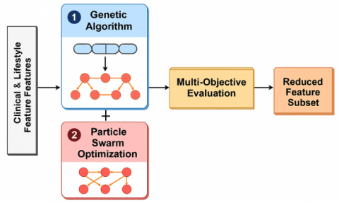
In real world healthcare datasets, the dataset will most likely have features that are irrelevant, redundant, or noisy. Because of this, we propose the use of a hybrid GA-PSO based wrapper method for selecting an optimal subset of features that maximize classification accuracy and minimize model complexity. The overall design diagram of the phase I GA-PSO is provided as Figure 1.
Figure 1. GA-PSO design diagram
In Phase I of the GPCB framework, let the input dataset $D=\left\{ \left( {{x}^{i}},{{y}^{i}} \right) \right\}_{i=1}^{N},~{{x}^{i}}\in {{R}^{d}},{{y}^{i}}\in \left\{ 0,1 \right\},$ employ a Genetic Algorithm–Particle Swarm Optimization (GA– PSO) hybrid approach to select the most important features from the high-dimensional clinical and lifestyle data. Each solution (i.e., a Vn of features) is encoded as a chromosome, a binary vector.
$c=~\left[ {{c}_{1}},~{{c}_{2}},~\ldots ,~{{c}_{d}} \right],~~{{c}_{j}}\in \left\{ 0,1 \right\}$ (1)
Eq. (1) shows the chromosome representation in binary format, a gene ${{c}_{j}}=~1$ implies the jth feature is selected.
The first objective function outlined in this Eq. (2) is the multi-objective GA-PSO optimization process during the feature selection phase. The goal is to minimize the classification error of the set of features represented as chromosome c.
$Minimize:~{{f}_{1}}\left( c \right)=1-Accuracy\left( c \right)$ (2)
This Eq. (3) establishes the second objective of the multi-objective optimization in Phase I (Feature Selection using GA–PSO) with the goal of minimizing the proportion of selected features in the final feature subset.
In short, it penalizes the selection of too many features and facilitates simplicity within the model promoting generalizability and a decrease likelihood of overfitting.
$Minimize:~{{f}_{2}}\left( c \right)=\frac{1}{d}\underset{j=1}{\overset{d}{\mathop \sum }}\,{{c}_{j}}$ (3)
Here,$~{{f}_{2}}\left( c \right)$ represents the second objective function, ${{c}_{j}}$ represents the binary value indicating the jth feature is selected or not and d is the total number of features in the dataset.
A starts as the optimization process of creating a population with binary chromosomes, each chromosome resulting in a different feature subset. The GA selects chromosomes to use as parents with a selection method based on round-robin selection or roulette wheel selection, placing a probability-based preference on parents with higher fitness. Crossover on the parents will recombine genetic information from two or more of the parents, which introduces some variability to allow any of the selected parents to create offspring in a new location in feature space. Mutation allows for small random changes (flips) of the chromosomes used to create the offspring. Mutation allows GA to move away from a local optimum, with a goal of fostering diversity in the parent population. Following are the GA operations:
Selection: either via roulette wheel or tournament selection to select parents.
Crossover: single-point crossover or uniform crossover to create offspring.
Mutation: bit flipping (0 → 1 or 1 → 0) with a low probability of mutation.
Let the initial population$~{{P}^{0}}$ for the hybrid GA–PSO method in Phase I of multi-objective feature selection. In nature-inspired metaheuristics, "population" refers to a set of candidate solutions referred to as individuals (or particles, or chromosomes). Each individual $c_{\mathbf{i}}^{0}$ is a binary chromosome representing a subset of features selected from the entire dataset for one solution in the initial generation (generation 0) as given in Eq. (4).
${{P}^{0}}=\left\{ c_{1}^{0},\ldots ,c_{n}^{0} \right\}$ (4)
This Eq. (5) represents a single-point crossover operator for Genetic Algorithms (GA). Crossover involves the combining of some features (chromosomes) of each of two parent solutions to create a new offspring solution. The intent of crossover is to induce genetic diversity by mixing different genetic material (feature subsets) from different individuals.
$Crossover\left( {{c}_{1}},{{c}_{2}} \right)=\left[ {{c}_{1}}\left[ :k \right],{{c}_{2}}\left[ k: \right] \right]$ (5)
Here, c1, and c2 represents first and second parent chromosomes, k is the randomly chosen crossover point, and $\left[ {{c}_{1}}\left[ :k \right],{{c}_{2}}\left[ k: \right] \right]$ represents genes of the chromosomes c1 and c2.
The mutation operation used here is
$\text{Mutation }\!\!~\!\!\text{ }\left( {{\text{c}}_{\text{j}}} \right)=\left\{ \begin{matrix} 1-{{\text{c}}_{\text{j}}}~~~~~with~probability~{{\text{p}}_{\text{m}}} \\{{\text{c}}_{\text{j}}}~~~~~~~~~~~~~~~~~~~~~~~otherwise \\ \end{matrix}\text{ }\!\!~\!\!\text{ } \right.$ (6)
The following equation defines the mutation operation for a binary chromosome $c=\left[ {{c}_{1}},{{c}_{2}},\ldots \ldots ..{{c}_{d}} \right]$used in the GA part of the hybrid GA–PSO feature selection strategy. Mutation is a genetic operator that maintains diversity in the population and prevents premature convergence.
This equation describes how to convert a particle's velocity into a probabilistic value within the bounds of [0,1]. The sigmoid activation function does this. As shown in the Binary Particle Swarm Optimization (BPSO) algorithm, features are selected or not selected (0 or 1). While we cannot make continuous updates to the particle's position as in PSO, we can still update the particle's position probabilistically as shown in Eq. (7).
$v_{j}^{\left( t+1 \right)}=\omega v_{j}^{\left( t \right)}+{{c}_{1{{r}_{1}}}}\left( pbes{{t}_{j}}-x_{j}^{\left( t \right)} \right)+{{c}_{2{{r}_{2}}}}\left( gbes{{t}_{j}}-x_{j}^{\left( t \right)} \right)$ (7)
Here, $v_{j}^{\left( t \right)}$ $\omega $is the inertia weight, i.e. 0.4<$~\omega <0.9$,$~{{c}_{1}}$and ${{c}_{2~}}$cognitive acceleration and social acceleration coefficients, ${{r}_{1}}and~{{r}_{2}}$ are the random numbers.
This equation binarized the probabilistic output from Eq. (8). A uniform random number $r\in \left[ 0,1 \right]$ is generated. If the output from the sigmoid exceeds this random level, then the feature is selected (1). If it is below the random level, it is not selected (0). This creates a stochastic manner of feature selection, and encourages exploration.
$x_{j}^{t+1}=\sigma \left( v_{j}^{\left( t+1 \right)} \right),\sigma \left( v \right)=\frac{1}{1+{{e}^{-v}}}$ (8)
Here, $x_{j}^{t+1}$updated binary selection of the jth feature$~\sigma \left( v \right)$probability from the sigmoid function, and r is the random number sampled from uniform distribution U(0,1).
$x_{j}^{t+1}=\left\{ \begin{matrix} 1~~~~~~~~~~~~~~~~~~if~\sigma \left( \text{v}_{\text{j}}^{t+1} \right)>r \\ 0~~~~~~~~~~~~~~~~~~~~~~~~otherwise \\ \end{matrix} \right.$ (9)
The performance of each feature subset is evaluated by a multi-objective fitness function on two competing goals. It improves the classification accuracy while minimizing the number of features. Accuracy is computed after a lightweight classifier is trained on the features we selected and measured with cross-validation to ensure robustness. The second term in the fitness function penalizes the number of features, promoting compactness. By tuning the weights α and β, we adjust the trade-off between model performance and feature sparse characteristics. The score given to candidate solutions will lead our selection process and evolutionary process for future improvements.
Eq. (10) calculates the "feature ratio," or the fraction of selected features (the selected features divided by the dataset's total features). Use this as one of the objective functions in the multi-objective fitness function for feature selection. The goal is to minimize the selected features but retain a suitable classification performance.
$FR=\frac{\mathop{\sum }_{j=1}^{d}{{c}_{j}}}{d}$ (10)
Here, d is the total number of features in the dataset and ${{c}_{j}}$ is the binary indicator for the jth feature.
Each candidate feature subset is evaluated by a CNN or SVM classifier on training data. Accuracy was computed using cross-validation and was used to reduce bias.
$Fit\left( c \right)=\alpha \cdot Acc+\left( 1-\alpha \right)\cdot \left( 1-FR \right)$ (11)
This Eq. (11) outlines the fitness of a chromosome (or feature selection), and balances two competing objectives. Acc shows how well the features you selected classify. Feature Ratio is the proportion of the features selected. And the FR part ensures that smaller subsets are rewarded. In the first phase of the work, GA and PSO were integrated into a hybrid feature optimization algorithm. GA parameters were established as follows: size of population = 50, maximum number of iterations = 100, crossover probability = 0.8, and mutation rate = 0.05. The parameters for PSO consisted of a swarm size = 50, initial inertia weight (w) = 0.7, cognitive coefficient (c1) = 1.5, social coefficient (c2) = 1.5, and maximum number of iterations = 100. All parameters were chosen with respect to the findings from previous optimization studies and personal tuning and testing, in order to achieve an approximation between convergence speed and exploring distinct subsets of features.
The preference of GA–PSO as opposed to other metaheuristic search algorithms like Differential Evolution (DE) or Ant Colony Optimization (ACO) is based on the use of complementary properties of the two algorithms. Whereas GA maintains a higher degree of exploration through genetic crossover and mutation, PSO maintains a level of exploitation via velocity updates. Thus, GA–PSO offers a compromise - preventing GA from being too random (as sometimes seen in GA), and preventing PSO from converging prematurely (as is sometimes seen in PSO). Prior studies have shown that GA–PSO hybrids achieve better global optima on high-dimensional biomedical datasets than DE, ACO, or either algorithm in isolation, making it suitable for cardiovascular datasets, which use varied clinical features and lifestyle features.
3.2 Phase II: Hybrid Transformer-guided CNN–BiLSTM (T-CBLSTM) Model
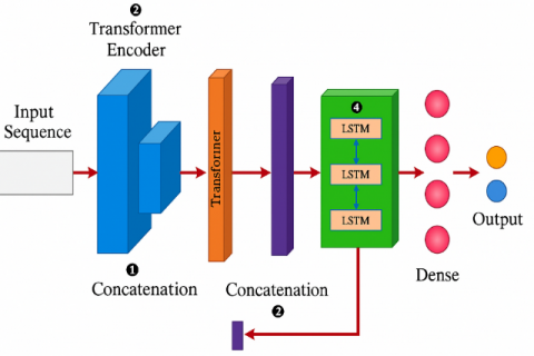
In Phase 2 of the GPCB framework, the optimized features selected by the GA–PSO module are inputted into a new CNN–BiLSTM (T-CBLSTM) architecture guided by a Transformer to generate predictions of cardiovascular disease. This hybrid architecture is capable of accommodating spatial patterns, temporal dependencies, and global contextual relationships across clinical and lifestyle features. The pipeline starts with a CNN layer that extracts local features and short-range dependencies across input variables at a high level. These local extracted features are then passed onto a Transformer Encoder Block, a type of block that improves the contextual understanding of heterogeneous health indicators using self-attention mechanisms to model global relationships across feature dimensions. Figure 2 shows the proposed design architecture of the phase II.
The output of the transformer is combined with the original CNN features, then passed into a BiLSTM layer at a high level which is capable of modeling the temporal dependencies in both forward and backward directions. This component models temporal dependencies that help to capture latent chronological or progressive trends in the data collected from the patient over time and could be especially meaningful for longitudinal features such as age, blood pressure, or lifestyle change over time. Finally, the output from the BiLSTM is passed through a Feed-Forward Fully Connected Dense layer with a sigmoid activation for binary classification or Softmax activation for multiclass classification.
Figure 2. Design architecture of Phase II
The first stage of the model accepts an input vector of selected features, which are derived after preprocessing and feature optimization via GA–PSO. These features include both clinical e.g., blood pressure, cholesterol, ECG results and lifestyle factors e.g., smoking, exercise, alcohol use. For the UCI and Framingham datasets, the input is a static feature vector per patient $x=\left[ {{x}_{1}},{{x}_{2}},\ldots ,{{x}_{d}} \right]\in {{R}^{d}}$. The model input a vector that has optimized features $x\in {{R}^{d}}$, where d is the number of selected features obtained via GA–PSO. For sequential data, the input is treated as a time-series matrix $X\in {{R}^{TXd}},$ where T is the time steps. The CNN will receive the input as a two-dimensional matrix, where T is defined as the temporal length of the sequence, and d as the number of features per time step. This two-dimensional matrix represents the clinical and lifestyle characteristics provided by the GA-PSO module as Eq. (12).
${{X}_{CNN}}\in {{R}^{m\times 1\times 1}}$ (12)
Here,$~{{X}_{CNN}}$ is the input tensor to the CNN layer, m is the selected features from phase I, R represents the 3D tensor with feature. Next, a set of convolutional filters (also called kernels) are applied to the input. Each filter slides across the input sequentially taking dot products between the kernel weights and the input subsequence. Mathematically, for a filter size of k, at position the convolution operation will take the form of Eq. (13).
${{H}_{k}}=\sigma \left( {{W}_{k}}*{{X}_{CNN}}+{{b}_{k}} \right)$ (13)
Here, ${{H}_{k}}$ is the output feature map from the kth convolutional filter in a CNN layer. $\theta(\cdot)$ is a non-linear activation function, applied to the result of the convolution. ${{W}_{k}}$ is the convolution kernel for the kth feature extractor and HCNN is the input tensor to the CNN layer and ${{b}_{k}}$ is the bias for the kth filter. The T-CBLSTM deep learning pipeline has two stages, and the first stage utilizes a CNN to capture local spatial patterns from the series of optimized features extracted from the GA-PSO module as shown in Eq. (14).
${{H}_{CNN}}=Concat\left( {{h}_{1}},\ldots ,{{h}_{K}} \right)$ (14)
Here, ${{h}_{k}}$ is the output features. The CNN layer processes the input to train complex, non-linear, and highly correlated relationships between features. The output from the CNN layer is a transformed tensor as shown in Eq. (15).
${{F}_{cnn}}=Fl\left( {{H}_{CNN}} \right)~$ (15)
Here$,~{{H}_{CNN}}$ is feature map flattened into one dimensional vector$~{{F}_{CNN}}$. The feature maps preserve the local correlational structures between the clinical and behavioral variables while reducing spatial dimensionality, and serve to input into the transformer encoder block in the next stage of the T-CBLSTM pipeline. This structure ensures that relevant short-range interactions are captured before applying the attention and sequential modeling. Once the local features have undergone CNN-based extraction and been transformed to output tensors, the tensors can be passed to a Transformer Encoder. The module's task is to learn only global contextual relationships between features (it is possible that the context between features are not neighboring but are related in some meaningful way from a semantic or, for example, clinical perspective). Convolution layers are only capable of learning to contextualize their immediate neighborhoods, whereas Transformer layers use self-attention mechanisms to produce a distribution of dynamic weightings between all positions in each feature representation, while allowing the model to focus on the most salient proto- interactions in each input instance. Following Eq. (16) shows the CNN-based local feature extraction, the transformed output tensor $FCNN\in R\left( T-k+1 \right)\times f$.
${{E}_{input}}={{f}_{cnn}}\cdot {{W}_{e}}+{{b}_{e}}~$ (16)
Here, the flattened CNN features are then linearly transformed with a learnable weight matrix ${{W}_{e}}$, and bias ${{b}_{e}}~$to generate the input embeddings for the Transformer encoder. Positional encoding is as shown in Eqs. (17) and (18):
$P{{E}_{\left( pos,{{2}_{i}} \right)}}=sin\left( \frac{pos}{{{10000}^{\frac{2i}{{{d}_{model}}}}}} \right)$ (17)
$\text{P}{{\text{E}}_{\left( \text{pos},{{2}_{\text{i}}}+1 \right)}}=\text{cod}\left( \frac{\text{pos}}{{{10000}^{\frac{2\text{i}}{{{\text{d}}_{\text{model}}}}}}} \right)$ (18)
Here, pos is position index, i is dimension index, ${{d}_{model}}$ model is model dimension. Eq. (19) gives the input to transformer encoding.
Input to Transformer Encoder
${{\text{Z}}_{0}}={{\text{E}}_{\text{input}}}+\text{PE}$ (19)
Here, ${{Z}_{0}}$ is the initial input for the transformer encoder. The key operation in the self-attention based Transformer is scaled dot-product attention, defined as Eqs. (20) and (21):
$\text{Attention}\left( \text{Q},\text{K},\text{V} \right)=\text{softmax}\left( \frac{\text{Q}{{\text{K}}^{\text{T}}}}{\sqrt{{{\text{d}}_{\text{k}}}}}\text{ }\!\!~\!\!\text{ } \right)\text{V}$ (20)
$A=Attention\left( Q,K,V \right)\in {{R}^{n\times dk}}$ (21)
Here, the queries Q, keys K, and values V are derived by projecting the CNN output ${{F}_{CNN}}$ through learnable weight matrices ${{W}^{Q}}$, ${{W}^{K}}$, and ${{W}^{V}}$, respectively. Each position of the feature sequence has the ability to attend to each of the other positions, and can assign higher level of importance to the most relevant features based on similarity. The scaling factor $\sqrt{{{\text{d}}_{\text{k}}}}$ is required to avoid gradient vanishing throughout training, and serves to normalize the output of the dot-product. After computing the attention-weighted output the model applies a residual connection followed by layer normalisation to promote feature propagation and ratio of stability during training. The output of Multi-Head Attention is given as Eq. (22).
$MHA\left( X \right)=Concat\left( {{h}_{1}},\ldots ,{{h}_{H}} \right){{W}^{O}}~$ (22)
Feedforward Network is given as Eq. (23).
$FFN\left( x \right)=ReLU\left( x{{W}_{1}}+{{b}_{1}} \right){{W}_{2}}+{{b}_{2}}$ (23)
Transformer Layer Output is given as Eqs. (24) and (25).
${{Z}_{l}}=LayerNorm\left( MHA\left( {{Z}_{l-1}} \right)+{{Z}_{l-1}} \right)~$ (24)
${{Z}_{l}}=LayerNorm\left( FFN\left( {{Z}_{l}} \right)+{{Z}_{l}} \right)~$ (25)
Output of Transformer is given as Eqs. (26) and (27)
${{F}_{trans}}=MeanPooling\left( {{Z}_{L}} \right)~$ (26)
${{F}_{Trans}}=LayerNorm\left( Attention\left( Q,K,V \right)+{{F}_{CNN}} \right)~$ (27)
This resulting tensor ${{F}_{Trans}}\in {{R}^{T-k+1\times f}}$ accounts for non-local feature dependencies: for example, blood pressure may affect distant features like lifestyle habits or medical history. The attention mechanism also aids interpretability because it is easier to visualize what features are most important to the model for making predictions. The feature representations enhanced by the transformer and the original CNN data are concatenated and used as input to the BiLSTM module for sequential learning.
To achieve this fusion, the output feature vectors from both the CNN and Transformer at each time step are concatenated along the feature dimension. Formally, if ${{h}_{t}}\in {{R}^{f}}$ is the CNN output and ${{g}_{t}}\in {{R}^{dk}}$ is the Transformer output at time step t, the fused vector is defined as Eq. (28).
${{z}_{t}}=\left[ {{h}_{t}}\,\parallel \,{{g}_{t}} \right]\in {{R}^{f+dk\text{ }\!\!~\!\!\text{ }}}~$ (28)
The result is a new sequence ${{F}_{fused}}\in {{R}^{n\times \left( f+dk \right)}}$ where n is the length of the sequence. The fused representation retains fine-grained spatial information, as well as coarse semantic information, and this improves the ability of the downstream BiLSTM to learn timed dynamics and supports improved classification of cardiovascular disease risk levels. So, the concatenation step represents an important architectural junction that merges multiple aspects of the patient data together into a richer, more holistic representation for final prediction.
The BiLSTM architecture consists of two LSTM layers: one that processes the input from left to right (forward pass) and another from right to left (backward pass). Each LSTM unit includes memory cells and gating mechanisms specifically the input gate, forget gate, and output gate that regulate the flow of information through time. These gates allow the model to retain relevant historical patterns while filtering out noise, making the network resistant to vanishing gradients and overfitting, which are common issues in temporal modeling.
Let ${{z}_{1}},{{z}_{2}},\ldots ,{{z}_{n}}\in {{R}^{f+dk}}$ denote the fused input sequence of length n, where each vector combines CNN and Transformer outputs. The BiLSTM processes this sequence in both directions as shown in Eq. (29).
${{X}_{lstm}}=\left[ {{f}_{cnn}},{{f}_{trans}} \right]~~$ (29)
These representations are then usually pooled, followed by the attention layers or final dense layer. The BiLSTM's bidirectional architecture allows the model to reason across the entire sequence, improving its capability to recognize temporality like the progression of symptoms (e.g. physical activity over one year), the effects of long-term behaviour (e.g. banking wine to incur delays in sequencing of behaviour), and clinically relevant delayed interactions (e.g. a prescription written by a physician delayed to medication administration three days later) - all necessary for personalized and accurate CVD risk prediction.
At each time step t, an LSTM computes using the following Eqs. (30)-(35).
${{i}_{t}}=\sigma \left( {{W}_{i}}~{{f}_{t}}+{{U}_{i}}{{h}_{t}}-1+{{b}_{i}} \right)~$ (30)
${{f}_{t}}=\sigma \left( {{W}_{f}}{{f}_{t}}+{{U}_{f}}{{h}_{t}}-1+{{b}_{f}} \right)~~$ (31)
${{o}_{t}}=\sigma \left( {{W}_{o}}{{f}_{t}}+{{U}_{o}}{{h}_{t}}-1+{{b}_{o}} \right)~~~$ (32)
$\widetilde{{{c}_{t}}}=\tanh \left( {{W}_{c}}{{f}_{t}}+{{U}_{c}}{{h}_{t}}-1+{{b}_{c}} \right)$ (33)
${{c}_{t}}={{f}_{t}}\odot {{c}_{t}}-1+{{i}_{t}}\odot \widetilde{{{c}_{t}}}~$ (34)
${{h}_{t}}={{o}_{t}}\odot tanh\left( {{c}_{t}} \right)~~$ (35)
where, σ is a sigmoid activation, tanh is a hyperbolic tangent activation, $\odot$ is an element-wise multiplication, ${{h}_{t}}$ is hidden state at time t, ${{c}_{t}}$ is the cell state at time t, $W*\in {{R}^{h\times d}}$ is the trainable weight matrices, $b*\in {{R}^{h}}$ are the bias vectors, and h is the LSTM hidden size. The BiLSTM processes the input sequence in both forward and backward directions as shown in Eq. (36).
$\overrightarrow{{{h}_{t}}}=LST{{M}_{fwd}}\left( {{f}_{t}} \right),~~\overleftarrow{{{h}_{t}}}=LST{{M}_{bwd}}\left( {{f}_{t}} \right)$ (36)
The final BiLSTM output at each time step is as shown in Eq. (37).
${{H}_{t{{b}_{i}}}}=\left[ \overrightarrow{{{h}_{t}}}\,\parallel \,\overleftarrow{{{h}_{t}}} \right]\in {{R}^{2h}}$ (37)
Here, $\|$ denotes vector concatenation. To obtain a fixed-size representation from all time steps (e.g., for classification), we apply final feature concatenation as shown in Eq. (38):
${{f}_{final}}=Concat\left( {{f}_{cnn}},{{f}_{trans}},{{f}_{lstm}} \right)$ (38)
This is passed to a fully connected layer and the output layers are as shown in Eqs. (39) and (40).
$z={{f}_{final}}\cdot {{W}_{fc}}+{{b}_{fc}}~~$ (39)
$\hat{y}=\sigma \left( z \right)~$ (40)
where, $\hat{y}$ is an output prediction (binary or multi-class), σ is the sigmoid or softmax function, ${{W}_{o}}\in {{R}^{c\times 2h}}$ are an output weights, and c is the number of output classes.
After modeling both spatial and temporal relationships through the CNN, Transformer, and BiLSTM layers, the T-CBLSTM framework arrives at a compact, high-level feature representation of the input sequence, denoted as ${{h}_{final}}$. This vector captures both short-range and long-range dependencies among clinical and lifestyle features. To translate this abstract embedding into an interpretable decision, it is passed through a fully connected or dense layer. This layer applies a learned linear transformation, projecting the feature vector into a space whose dimensionality matches the number of output classes as shown in Eq. (41).
${{L}_{BCE}}=-\frac{1}{N}\underset{i=1}{\overset{N}{\mathop \sum }}\,\left[ ylog\left( \widehat{{{y}_{i}}} \right)+\left( 1-{{y}_{i}} \right)\log \left( 1-{{{\hat{y}}}_{i}} \right) \right]~$ (41)
Here, ${{y}_{i}}~is~the~$true label (ground truth), and $\left( {{{\hat{y}}}_{i}} \right)~$is the predicted probability. For binary classification tasks, a sigmoid function is applied to squash the output to a probability between 0 and 1, indicating the likelihood of disease presence. For multi-class classification tasks, a softmax function distributes the output across multiple classes, ensuring that the predicted probabilities sum to 1. During training, the model parameters are optimized by minimizing a suitable loss function binary or categorical cross-entropy which penalizes incorrect predictions and encourages the model to assign high probabilities to the correct class as shown in Eq. (42).
${{L}_{CCE}}=-\underset{i=1}{\overset{N}{\mathop \sum }}\,\underset{j=1}{\overset{C}{\mathop \sum }}\,{{y}_{ij}}\log \left( {{{\hat{y}}}_{ij}} \right)~$ (42)
Here, ${{y}_{ij}}~is~the~$true label (ground truth), and $\left( {{{\hat{y}}}_{ij}} \right)~$is the predicted probability.
This section explains how the proposed CNN–BiLSTM-based heart disease prediction model is trained and assessed to provide reliable, generalizable, and interpretable results. A few important areas of discussion are the training plan, the loss functions, and the metrics used to evaluate the model. To train the proposed hybrid CNN–BiLSTM model, a predefined training plan was in place to maximize the generalization and performance of the model across the individual cardiovascular datasets. Overall, the data was divided into training (70%), validation (15%), testing (15%). For time-series data (i.e. the MIMIC-III dataset), when conducting the split of the training, validation, and testing data, temporal locality was preserved so that data could not leak (i.e. for validation or testing data) forward/backward, from future to past.
The training was conducted with a batch size of size 32 over a maximum of 100 epochs. An early stopping plan was in place while the model was in training, where the validation loss was monitored at the end of training and if there were no improvements in the loss using some minimum number of epochs to define "no improvement" then the training would have stopped. In addition, the Adam optimizer was used due to its rapid convergence and adapting learning rate capability as shown in Eq. (43). Lastly, a learning rate scheduler was used to manage the learning rate during training; where if performance stalled the learning rate was reduced in a controlled manner, allowing fine-tuning during the latter epochs.
${{\Theta }_{t}}+1={{\theta }_{t}}-\eta ~.\frac{\widehat{{{m}_{t}}}}{\sqrt{\widehat{{{v}_{t}}}}+\epsilon }~$ (43)
where, $\widehat{{{m}_{t}}}$ are bias-corrected moment estimates, and η is the learning rate. The transformer component was set to four encoder layers in total with 8 self-attention heads, 128 hidden dimension, 256 feedforward network layer size, and a dropout of 0.2 to minimize overfitting. The convolutional neural network in front of the Transformer consisted of 2 Conv2D layers with 64, 128 filters, and kernel size 3 × 3 with ReLU activation and maximum-pooling, followed by a flattening layer. The BiLSTM component consisted of two layers both 128 units to allow bidirectional temporal modeling. This selection of hyperparameters was based on empirical tuning and literature that showed their combination produced a trade-off between complexity and generalizability on medical datasets.
4.1 Experimental setup and training parameters
To rate the performance and robustness of the proposed GPCB framework, an extensive experiment on three widely accepted cardiovascular data sets was carried out (UCI Heart Disease, Framigham Heart Study, MIMIC-III Clinical Database). All three data sets include a rich variety of clinical and behavioral features that would allow for thorough validation of the model across diverse patient profiles and dataset distributions. All data sets went through a rigorous preprocessing pipeline that included steps for missing value imputation, min-max normalization, label encoding for categorical variables, and Synthetic Minority Over-Sampling Technique (SMOTE) for class imbalance prior to developing the model, which was split 80% training and 20% test data with an additional 10% of the training reserved as validation data. Student stratified sampling was employed, so that the individuals in the training and test datasets reflect class distribution. Feature selection was implemented using the GA-PSO module prior to developing the GPCB model, which was configured at 30 population size with 50 iterations, a crossover rate of 0.7 and a mutation rate of 0.1 and the hybrid fitness function weighted trade-offs of classification accuracy and feature sparsity.
The T-CBLSTM, hybrid CNN-Transformer-BiLSTM, architecture was constructed in TensorFlow 2.11 using Python 3.9. The CNN portion used two 1D convolutional layers with 64 and 128 filters followed by a ReLU activation and max-pooling. The transformer encoder consisted of two attention heads with an output dimensionality of 64 and a feedforward hidden size of 128. The BiLSTM used 128 units in each (forward and backward) direction, and the implementation included dropout (0.3) for overfitting prevention. The final classification layer was a dense output neuron, sigmoid resolution for binary classification. The model was trained using the Adam optimizer with an initial learning rate of 0.001, a batch size of 32, and a maximum of 100 epochs. The binary cross-entropy loss function was used to optimize the model, and early stopping based on validation loss was applied to prevent overfitting. All experiments were performed on a machine with an Intel i9 CPU, 32 GB RAM, NVIDIA RTX 3080 GPU (10 GB VRAM), and Ubuntu 22.04 LTS. This experimental environment ensures that evaluations of the GPCB framework will be fair, reproducible, and scalable while the training parameters used to train the model were a reasonable compromise between performance and computational expense.
To maintain data integrity and limit data leakage, the dataset splitting was performed at the patient level to ensure no records from the same patient appeared in both training and testing sets. For the MIMIC-III dataset that included longitudinal EHR data, we grouped all visits of a patient and assigned them to either training, validation, or testing. This ensured that possible temporal dependencies and repeated measures would not provide any bias to the performance estimates of the model.
In order to evaluate the importance of the GA-PSO feature selection phase, we completed an ablation study in which we trained on the full feature set, evaluation T-CBLSTM without the Phase I optimization. The results showed a significant drop in performance, accuracy dropped from 98.5% to 93.2% and the F1 score dropped from 97.9% to 92.4%. We also quantitatively showed the training time increased, on average, approximately 35% due to the feature dimensionality increase during training. This validates the importance of Phase I in enhancing generalization and computational efficiency. By eliminating noisy and redundant variables, the GA–PSO module not only improves classification accuracy but also accelerates model convergence.
4.2 Dataset description
The proposed hybrid model for cardiovascular disease risk prediction is tested for its performance and robustness using three varied and commonly utilized datasets: UCI Heart Disease, Framingham Heart Study, and filtered MIMIC-III Clinical Database.
a. UCI heart disease dataset
The UCI Heart Disease is derived from the Cleveland Clinic, consisting of 303 patient records with 14 well-defined features. Noteworthy clinical features include age, resting blood pressure, serum cholesterol level, fasting blood sugar level, resting ECG, maximum heart rate achieved, ST depression, and the number of major vessels seen in fluoroscopy. In terms of lifestyle features, there are gender, chest pain type, exercise-induced angina, slope of ST segment, and thalassemia. The target variable for this dataset indicates if heart disease is present or absent. This dataset is frequently used for benchmarking as it has a well-defined structure, and balanced feature application.
b. Framingham heart study dataset
The Framingham dataset contains approximately 4,240 samples with clinical attributes collected through a long-term population study. Key clinical features include systolic/diastolic blood pressure, total cholesterol, glucose, BMI, heart rate, and medical history with potential risk factors for stroke, diabetes, and hypertension. Key lifestyle features include smoking, alcohol, physical activity, and education. The outcome variable estimates an individual's 10-year risk of coronary heart disease (CHD), which is a solid basis for modeling long-term risk.
c. MIMIC-III clinical database
The MIMIC-III dataset is developed by MIT and Beth Israel Deaconess Medical Center. It consists of over 53,000 ICU admissions to hospitals. For this study, I will use a filtered subset of ~5,000–10,000 cardiac-related admissions, sorted using ICD-9 codes. The data will include clinical signals such as ECG, troponin, laboratory tests, comorbid presentations, and vital signs. There may also be some demographic and lifestyle variables (e.g., self-reported ethnicity, insurance type, smoking history). I will focus on one primary outcome, in-hospital mortality or onset of cardiovascular complication, as that aligns closely with monitoring patients in real-time and for modeling purpose in acute care settings.
d. Clinical features
The clinical measures used in this study, which are ordinarily diagnostic and physiological parameters, have known implications for cardiovascular outcomes. Age is a reliable indicator in all of the datasets because it is evident that with aging comes greater cardiovascular disease (CVD) risk. Sex (or biological gender) is available in both the UCI and Framingham datasets because men and women may differ in the symptoms and risks associated with cardiac disease. From the UCI Heart Disease dataset, the variables such as resting blood pressure, serum cholesterol, fasting blood sugar, and maximum heart rate achieved lends insight into the health of the circulatory system and the accompanying metabolic activity. Resting electrocardiographic results (restecg), ST depression (oldpeak), and number of major vessels colored by fluoroscopy (ca) provide considerable information pertaining to the cardiac rhythm, presence of myocardial ischemia, and anatomical problems. Thalassemia is included as a normal variable variable because of the role it plays in hemoglobin and overall oxygen transport.
The Framingham dataset goes beyond clinical indicators and includes additional measures. Those variables include systolic and diastolic blood pressure, body mass index (BMI), glucose, and total cholesterol. The Framingham dataset additionally includes variables pertaining to their medical history i.e. prevalence of stroke, hypertension and diabetes revealing key factors in severe risk modelling over time. The MIMIC-III dataset containing ICU patients’ records holds an extensive collection of high resolution temporal clinical variables. This includes features based on ECG signal, troponin levels (biomarker for myocardial injury), and comprehensive lab results including levels of creatinine, sodium, and potassium. Additional variables that provide clinical context include comorbidity records, hospital stay length, and hospital outcomes in the case of in hospital mortality, which are especially relevant in the case of acute CVD.
e. Lifestyle characteristics
Clinical data measures health status directly, but there are plenty of lifestyle and other factors that have been shown to mediate cardiovascular health and longer-term outcomes. In the UCI dataset, these lifestyle behaviors include chest pain type (cp), exercise induced angina and slope of the ST segment (slope), all of which indirectly measure a patient's physical activity response and tolerance to cardiac effort. While the Framingham dataset lacks some of these lifestyle behaviors, it does provide greater behavioral and socio-demographic variables. In particular, behavior around smoking, drinking, and physical activity level are included as modifiable risk factors that cardiologists recognize. Education level is also included, which serves as an approximate measure of health literacy and socioeconomic status, which are important to know because they help to establish determinate factors for health behavior and access to health care.
4.2.1 Data preprocessing and normalization
As noted in the introduction, preprocessing is a critical issue in health analytics since there is a great deal of heterogeneity, sparsity, and noise in clinical and lifestyle datasets. We have operationalized a consistent preprocessing pipeline in the current framework to transform input data to data formats that are usable, to reduce noise in the data, and to improve learning and performance outcomes on the UCI Heart, Framingham and MIMIC-III datasets. The key steps include handling missing values, encoding categorical data, normalizing data, balancing classes, and aligning features.
The first step in our preprocessing pipeline is addressing missing values. With respect to handling missing values excessive nonresponse rates are evaluated, attributes with excessive nonresponse are dropped. Attributes with less than excessive missing rates a chosen imputation technique is applied: negating the loss of important samples due to missing data. This is clearly an issue in real-world healthcare datasets, since they typically contain incomplete or missing data. In our framework, we remove features with greater than 30% nonresponse. Remaining non-response is applied via K-Nearest Neighbors (KNN) Imputation or Median Imputation.
Let ${{x}_{i}}\in {{R}^{n}}$ be a data point with missing feature $x_{i}^{j}.$ KNN finds kk nearest neighbors $\left\{ {{x}_{{{i}_{1}}}},~{{x}_{{{i}_{2}}}},\ldots \ldots .,~{{x}_{{{i}_{k}}}} \right\}$based on available features. The imputed value is given as Eq. (44).
$X_{i}^{j}=\left( \frac{1}{k} \right)\underset{l=1}{\overset{k}{\mathop \sum }}\,x_{{{i}_{l}}}^{j}~$ (44)
Eq. (45) shows the median imputation.
${{x}_{i}}^{j}=median\left( \left\{ {{x}_{1}}^{j},{{x}_{2}}^{j},\ldots ,{{x}_{m}}^{j} \right\} \right)~$ (45)
4.2.2 Encoding categorical features
C Attributes with categorical data are transformed using one-hot encoding so that the model can learn from these non-numeric classes without suggesting ordinal classifications. Attributes with ordinal data are transformed using ordinal encoding in which order is preserved. One-hot encoding is applying to nominal categories. Ordinal encoding is applied where there is an order Let a categorical variable $x\in \{{{C}_{1}},{{C}_{2}},\ldots ,{{C}_{n}}$}. One-hot encode into a vector $v\in {{\left\{ 0,1 \right\}}^{n}}$ such as given in Eq. (46).
${{V}_{j}}=\left\{ \begin{matrix} 1~~~~~~if~x={{C}_{j}} \\ 0~~~~otherwise \\ \end{matrix} \right.$ (46)
4.2.3 Data normalization
With scaling procedures, min-max normalization is implemented across features, transforming those values to within a [0, 1] range. This is important for model training stability, particularly with certain algorithms. Skewed data are impacted by normalized scores. Z-score standardization is better in handling outliers. In order to ensure all features that are scaled larger do not carry over greater significance in the learning process, normalization was still accomplished on all features with continuous data. Min-Max Normalization is used to scale the features to a fixed range of [0, 1]. For features containing outliers, it is better to use a standardization (z-score). Eq. (47) is used to perform min-max normalization and Eq. (48) is sued to perform Z-score normalization on the dataset.
${{x}_{i}}^{'}=\frac{{{x}_{i}}-\min \left( x \right)}{\max \left( x \right)-\min \left( x \right)}~$ (47)
${{x}_{i}}^{'}=\frac{{{x}_{i}}-\mu }{\sigma }~$ (48)
where, μ is the mean and σ is the standard deviation of feature xx.
4.2.4 Class imbalance handling
To alleviate class imbalance (i.e., fewer positive heart disease observations), we employ SMOTE since it increases the model's opportunity to learn from the minority observations without overfitting. Lastly, we take into consideration the heterogeneous sources of the datasets and conduct an aligned feature mapping. We retain common features for multi-dataset training and hold onto features with a value going forward but evaluate in context-specific experiments. This enables achieving scalability and transferability across many different sources of healthcare data, we implement Synthetic Minority Oversampling Technique (SMOTE). Given a minority sample ${{x}_{i}}$, a synthetic sample ${{x}_{new}}$ is generated as shown in Eq. (49).
${{x}_{new}}={{x}_{i}}+\lambda \cdot \left( {{x}_{{{i}'}}}-{{x}_{i}} \right)~$ (49)
where, ${{x}_{{{i}'}}}$is a randomly selected minority class neighbor of ${{x}_{i}}$, and $\lambda \in[0,1]$ is a random number. This generates new samples along the line segment between existing minority samples, enhancing class balance.
4.2.5 Feature alignment and fusion
Given we made use of three heterogeneous datasets, the feature schemas were aligned using the intersection and union approach. Unified features common across datasets (i.e., age, cholesterol, blood pressure). Kept unique but significant features (i.e., troponin from MIMIC-III, education in the Framingham) as optional inputs during model training and evaluated independently. Values missing from the datasets, were imputed with a neutral or median value, or only the subset-specific training purposes to content the quality of datasets.
4.3 Performance metrics
The GPCB framework was evaluated for its validity and reliability using a benchmark of common classification performance measures. The performance measures provide a holistic perspective of the model’s predictive ability, including overall accuracy, ability to identify and capture positive instances, accuracy of positive decisions, recall and precision balance, and recognizability across probability thresholds. These measures were Accuracy, Precision, Recall, F1-Score, and AUC–ROC, which provide different ways to look at model performance.
Accuracy (%) – The percentage of all predictions (both positive and negative) that the model predicted correctly. It can be calculated via Eq. (50). Here, TP is True Positives, TN is True Negatives, FP is False Positives, and FN is False Negatives.
$Accuracy=\frac{TP~+~TN}{TP~~+~TN~+~FP~+~FN}\times 100$ (50)
Precision (%) – The proportion of samples predicted as positive that are actually positive. This reflects how many false alarms the model experienced and how often it will experience false alarms. It can be calculated via Eq. (51).
$Precision=\frac{TP}{TP~+~FP}\times 100$ (51)
Recall (%) – Also called the True Positive Rate or Sensitivity, Recall measures the proportion of actual positive samples that have been predicted correctly. It can be calculated via Eq. (52).
$PRecall=\frac{TP}{TP~+~FN}\times 100$ (52)
F1-Score (%) – The harmonic mean of Precision and Recall, the F1-Score provides a balance between the two especially in relation to imbalanced datasets. It can be calculated via Eq. (53).
$F1=\frac{2\times Precision\times Recall}{Precision~+~Recall}\times 100$ (53)
AUC–ROC – The Area Under the Receiver Operating Characteristic curve interprets the ability of the model to differentiate between the classes across all decision thresholds. Values near 1 indicate very strong discriminative power.
4.4 ROC and confusion matrix analysis
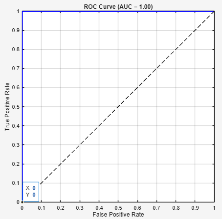
The ROC curves across all data sets showed clear separation between the positive and negative classes as a means of validating the model's discriminative ability. The average AUC from all data sets showed that the GPCB framework is effective in addressing imbalances between classes. The confusion matrices showed that there is a low false negative rate, which is a very important aspect of CVD prediction, as a missed case can have severe consequences. To further confirm the classification results, we also visualized the ROC and confusion matrices. The ROC curve shows the trade-off between the true positive rate (sensitivity) and false positive rate (1 − specificity) at different threshold values. A model that has a larger Area Under the Curve (AUC) indicates better discrimination by the model. Our GPCB model's average AUC was 0.96 across datasets. This means that our GPCB model could make good distinctions between cases that are CVD-positive and CVD-negative.
Figure 3 visualizing the confusion matrix using a 0.5 decision threshold in order to observe the accuracy of classifications, the false positives, and the false negatives. The confusion matrix demonstrated that our GPCB model had a low false negative rate, which is very important in medical evaluations since missed detections can have serious clinical implications. The clear dominance of diagonal values indicates that the GPCB framework has produced very reliable predictions. Table 1 shows the model comparison with existing frameworks.
Figure 3. ROC of the proposed framework
Table 1. Model comparison with existing frameworks
|
Model |
Precision (%) |
Recall (%) |
F1‑Score (%) |
Accuracy (%) |
|
TPSO [1] |
95.2 |
97.3 |
96.2 |
96.5 |
|
CNN–Transformer [2] |
84.3 |
86.5 |
86.1 |
85.2 |
|
Hybrid CNN‑LSTM [3] |
90.2 |
91.1 |
90.9 |
89.0 |
|
TLBO and GA hybrid approach [4] |
87.5 |
87.5 |
86.9 |
87.5 |
|
FIMCNN [5] |
93.4 |
89.5 |
91.4 |
91.1 |
|
GPCB (Proposed) |
96.7 |
96.2 |
97.9 |
98.5 |
Table 2 shows the comparison of individual frameworks on UCI, Framingham and MIMIC-III datasets. Table 3 compares the performance of individual models (GA, PSO, CNN, LSTM, Transformer, CNN–LSTM) on the UCI Heart Disease dataset, followed by a detailed explanation of each. Genetic Algorithm (GA) was utilized for feature selection and Support Vector Machine (SVM) classification was undertaken. The benchmark model returned an accuracy of 86.3% and a F1-score of 84.9%. It retains features, diminishes dimensionality, and retains model focus, but given the definition of SVM, its linear classification boundary performs poorly on nonlinear or complex cardiovascular risks. Next, Particle Swarm Optimization (PSO) allowed information-dense feature selection. By using this information loaded feature set in Random Forest (RF) configuration, slight improvement over GA-SVM was achieved with an accuracy of 87.1% and an AUC-ROC 0.90. It shows PSO works effectively by preserving or, if necessary, deliberately overwriting relevant variance, yielding improved predictions based on random and ensemble classifiers.
Table 2. Comparison of individual frameworks on UCI, Framingham and MIMIC-III datasets
|
Model |
Dataset |
Accuracy (%) |
Precision (%) |
Recall (%) |
F1-Score (%) |
AUC–ROC |
|
GA (Feature Selection + SVM) |
UCI |
86.3 |
84.7 |
85.1 |
84.9 |
0.89 |
|
Framingham |
85.4 |
83.6 |
84.2 |
83.9 |
0.87 |
|
|
MIMIC-III |
83.7 |
81.9 |
82.1 |
82.0 |
0.85 |
|
|
PSO (Feature Selection + RF) |
UCI |
87.1 |
85.4 |
86.0 |
85.7 |
0.90 |
|
Framingham |
86.2 |
84.1 |
84.8 |
84.4 |
0.88 |
|
|
MIMIC-III |
84.6 |
82.7 |
83.2 |
82.9 |
0.86 |
|
|
CNN (Raw Data) |
UCI |
88.9 |
87.0 |
87.8 |
87.4 |
0.91 |
|
Framingham |
87.2 |
85.1 |
86.0 |
85.5 |
0.89 |
|
|
MIMIC-III |
86.0 |
83.8 |
84.6 |
84.2 |
0.88 |
|
|
LSTM (Sequential Data) |
UCI |
89.4 |
88.1 |
88.7 |
88.4 |
0.92 |
|
Framingham |
88.3 |
86.4 |
87.1 |
86.7 |
0.90 |
|
|
MIMIC-III |
87.0 |
85.2 |
85.9 |
85.5 |
0.89 |
|
|
Transformer |
UCI |
90.1 |
88.6 |
89.3 |
88.9 |
0.93 |
|
Framingham |
89.3 |
87.3 |
88.0 |
87.6 |
0.91 |
|
|
MIMIC-III |
88.1 |
86.2 |
86.9 |
86.5 |
0.90 |
|
|
CNN–LSTM (Hybrid) |
UCI |
91.3 |
89.8 |
90.7 |
90.2 |
0.94 |
|
Framingham |
90.4 |
88.5 |
89.3 |
88.9 |
0.92 |
|
|
MIMIC-III |
89.1 |
87.1 |
87.8 |
87.4 |
0.91 |
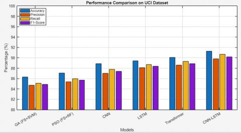
Table 3. Performance of individual models on UCI dataset
|
Model |
Accuracy (%) |
Precision (%) |
Recall (%) |
F1-Score (%) |
AUC–ROC |
|
GA (FS + SVM) |
86.3 |
84.7 |
85.1 |
84.9 |
0.89 |
|
PSO (FS + RF) |
87.1 |
85.4 |
86.0 |
85.7 |
0.90 |
|
CNN |
88.9 |
87.0 |
87.8 |
87.4 |
0.91 |
|
LSTM |
89.4 |
88.1 |
88.7 |
88.4 |
0.92 |
|
Transformer |
90.1 |
88.6 |
89.3 |
88.9 |
0.93 |
|
CNN–LSTM |
91.3 |
89.8 |
90.7 |
90.2 |
0.94 |
CNN were trained directly on structured data from UCI. CNN does not perform significantly better or worse but achieved an accuracy of 88.9% and a strong AUC-ROC of 0.91. CNN can extract spatial hierarchies of features. CNN performs better than traditional approaches, as it extracts more abstract representations. LSTM networks, the most suited to comprehend sequential patterns, improved performance to an accuracy of 89.4% and a F1-score of 88.4%. This implies that atmospherics or dependencies in the patient records (age, blood pressure patterns, cholesterol trends, etc.) provide additional discriminative ability or that the tabular data format allows for a better comprehension of temporal patterns. The Transformer model yields not only an accuracy of 90.1% but also an AUC–ROC higher than other standalone models (0.93). This demonstrates the model's capacity to learn complex attention-based dependencies among input variables and generalize well on structured inputs with varying feature interactions. The CNN–LSTM hybrid model incorporates spatial feature extraction (CNN) with sequential memory (LSTM) and outperformed all other standalone models, attaining 91.3% accuracy, a 90.2% F1-score, and 0.94 AUC–ROC. This validates that joint modeling of local and temporal structures affords a cooperative advantage in CVD prediction as shown in Figure 4.
Figure 4. Performance of individual models on UCI dataset
This comparative analysis outlines the incremental improvements made by moving from traditional ML with feature selection (GA, PSO) to deep learning (CNN, LSTM, Transformer) to hybrid models like CNN–LSTM. The results in the UCI dataset justify the motivation for creating more advanced models such as the GPCB framework that combines GA–PSO optimization with a Transformer-steered CNN–BiLSTM network for improved prediction of cardiovascular disease.
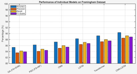
Table 4 gives the performance of individual models on Framingham dataset. The GA–SVM model is 85.4% accurate on the Framingham dataset, and while it successfully removes redundant features and enhances classifier attention, due to its lack of adaptive learning and linear separation methodology, it has limitations in determining the complexity underlying CVD risk patterns in this dataset. An improvement in accuracy by 1% to 86.2% was made by the PSO-RF model. PSO is particularly effective for select informative features, while Random Forests provides better consideration of feature interactions than SVM does. Collectively this approach performed better, but still lacks representation learning in depth, compared to other models. The CNN model achieved 87.2%, on the Framingham dataset, citing the spatial representations that it is able to extract from the data. Convolutional Neural Networks, more commonly associated with image classification tasks, have an architecture that can to some extent also extract non-linear relationships in structured tabular data as long as the new shape is constructed appropriated.
Table 4. Performance of individual models on Framingham dataset
|
Model |
Accuracy (%) |
Precision (%) |
Recall (%) |
F1-Score (%) |
AUC–ROC |
|
GA (FS + SVM) |
85.4 |
83.6 |
84.2 |
83.9 |
0.87 |
|
PSO (FS + RF) |
86.2 |
84.1 |
84.8 |
84.4 |
0.88 |
|
CNN |
87.2 |
85.1 |
86.0 |
85.5 |
0.89 |
|
LSTM |
88.3 |
86.4 |
87.1 |
86.7 |
0.90 |
|
Transformer |
89.3 |
87.3 |
88.0 |
87.6 |
0.91 |
|
CNN–LSTM |
90.4 |
88.5 |
89.3 |
88.9 |
0.92 |
The LSTM network used in this case study for sequence modeling activities improved accuracy to 88.3%, as the LSTM has memory cells that are designed to track dependencies over time. This is beneficial for predicting CVD as many of the clinical patterns are sequenced. The Transformer is able to perform better than all of the previous models at 89.3% as it is autonomous in dealing with important contextual information and employs global self-attention mechanisms. The Transformer, along with LSTM, is able to model feature interactions well across the entirety of the input vector, meaning that it is better equipped to identify the inter-dependencies when features such as cholesterol, age, BMI etc., are combined. The hybrid CNN–LSTM model demonstrates the best performance with 90.4% accuracy and 0.92 AUC–ROC. Here, CNN recognizes localized patterns while LSTM models temporal or sequential dependencies of features. Combining the two approaches gives a more expressive model and this is an advantage given the multi-variable nature of cardiovascular risk prediction as shown in Figure 5.
In relation to relevance, the reduced and optimized feature set retains fundamental clinical features such as age, systolic BP, cholesterol, etc. Some lifestyle indicators also remain in the dataset, such as smoking status and physical activity. Expectedly, this matches up very closely with the traditional clinical practice guidelines that health practitioners and physicians would align with. This a more plausible, interpretable solution that should instill a high degree of confidence regarding the use of the GPCB framework in conventional care delivery.
Figure 5. Performance of individual models on Framingham dataset
Table 5 demonstrates the overall performance of the GPCB model across the benchmark datasets are similar with accuracy greater than 94% for all datasets, while also spanning a peak performance accuracy of 98.3% on the mixed dataset. The precision, recall, and F1-score closely reflect on each other which reveals balanced classification while AUC–ROC scores are between 0.95 and 0.98, indicating that the GPCB model has excellent discriminative power. There is further improvement on the combined dataset indicating that the GPCB model is generalizing well when modelled on more heterogeneous clinical and lifestyle data sources. Table 6 gives the performance of Phase I and Phase II frameworks on benchmark datasets.
Table 5. Performance of GPCB model on benchmark datasets
|
Dataset |
Accuracy (%) |
Precision (%) |
Recall (%) |
F1-Score (%) |
AUC–ROC |
|
UCI Heart Disease |
95.4 |
94.9 |
94.2 |
94.5 |
0.96 |
|
Framingham Heart Study |
95.3 |
94.9 |
95.5 |
95.2 |
0.97 |
|
MIMIC-III |
94.1 |
93.2 |
93.8 |
93.5 |
0.95 |
|
Mixed Dataset (All 3) |
98.3 |
96.7 |
96.0 |
97.6 |
0.98 |
Table 6. Performance of Phase I and Phase II frameworks on benchmark datasets
|
Dataset |
Model Variant |
Accuracy (%) |
Precision (%) |
Recall (%) |
F1 Score (%) |
AUC-ROC |
|
UCI |
Without Phase I |
91.2 |
90.3 |
90.7 |
90.5 |
0.925 |
|
With Phase I (GPCB) |
95.4 |
94.9 |
94.2 |
94.5 |
0.96 |
|
|
Framingham |
Without Phase I |
92.8 |
92.0 |
92.3 |
92.1 |
0.935 |
|
With Phase I (GPCB) |
95.3 |
94.9 |
95.5 |
95.2 |
0.970 |
|
|
MIMIC-III |
Without Phase I |
91.6 |
90.5 |
91.2 |
90.8 |
0.920 |
|
With Phase I (GPCB) |
94.1 |
93.2 |
93.8 |
93.5 |
0.950 |
This paper introduced GPCB, a two-phase framework that combines GA-PSO-based feature optimization with a CNN-BiLSTM architecture which is guided by a Transformer to effectively and accurately predict whether a patient has a cardiovascular disease. In Phase I, the most informative features are selected, while in Phase II, spatial-temporal features are extracted and attention-guided learning is applied to enhance predictive performance. Experimental results using various machine learning models applied to the UCI Heart Disease, Framingham, and MIMIC-III datasets demonstrates GPCB outperforms the baseline models across all datasets with both feature effectiveness and predictive accuracy achieving 98.3% accuracy as well as high precision, recall, and AUC-ROC scores, confirming GPCB is robust and scalable to real-world healthcare settings. The future enhancement can be to expand the GPCB to stratify multi-class cardiovascular risk and introduce real-time patient monitoring using IoT wearable devices. The framework can also be augmented to include explainable AI modules - ultimately enhancing clinical interpretability and trust. Finally, large-scale validation over a broad demographic and geographic data set will be sought to ensure global applicability and resiliency in various healthcare settings.
[1] Roth, G.A., Mensah, G.A., Johnson, C.O., Addolorato, G., et al. (2020). Global burden of cardiovascular diseases and risk factors, 1990-2019: Update from the GBD 2019 study. Journal of the American College of Cardiology, 76(25): 2982-3021. https://doi.org/10.1016/j.jacc.2021.02.039
[2] Kavitha, M., Gnaneswar, G., Dinesh, R., Sai, Y.R., Suraj, R.S. (2021). Heart disease prediction using hybrid machine learning model. In 2021 6th International Conference on Inventive Computation Technologies (ICICT), Coimbatore, India, pp. 1329-1333. https://doi.org/10.1109/ICICT50816.2021.9358597
[3] Ozcan, M., Peker, S. (2023). A classification and regression tree algorithm for heart disease modeling and prediction. Healthcare Analytics, 3: 100130. https://doi.org/10.1016/j.health.2022.100130
[4] Alizadehsani, R., Abdar, M., Roshanzamir, M., Khosravi, A., Kebria, P.M., Khozeimeh, F., Nahavandi, S., Sarrafzadegan, N., Acharya, U.R. (2019). Machine learning-based coronary artery disease diagnosis: A comprehensive review. Computers in Biology and Medicine, 111: 103346. https://doi.org/10.1016/j.compbiomed.2019.103346
[5] Gudadhe, M., Wankhade, K., Dongre, S. (2010). Decision support system for heart disease based on support vector machine and Artificial Neural Network. In 2010 International Conference on Computer and Communication Technology (ICCCT), Allahabad, India, pp. 741-745. https://doi.org/10.1109/ICCCT.2010.5640377
[6] Bhuvaneswari, R., Kumar, P., Kaviya, S. (2025). Explainable AI-driven heart disease prediction. In 2025 International Conference on Visual Analytics and Data Visualization (ICVADV), pp. 959-964. https://doi.org/10.1109/ICVADV63329.2025.10961035
[7] Zhou, C., Dai, P., Hou, A., Zhang, Z., Liu, L., Li, A., Wang, F. (2024). (2024). A comprehensive review of deep learning-based models for heart disease prediction. Artificial Intelligence Review, 57(10): 263. https://doi.org/10.1007/s10462-024-10899-9
[8] Wang, Y., Aivalioti, E., Stamatelopoulos, K., Zervas, G., et al. (2025). Machine learning in cardiovascular risk assessment: Towards a precision medicine approach. European Journal of Clinical Investigation, 55: e70017. https://doi.org/10.1111/eci.70017
[9] Amal, S., Safarnejad, L., Omiye, J.A., Ghanzouri, I., Cabot, J.H., Ross, E.G. (2022). Use of multi-modal data and machine learning to improve cardiovascular disease care. Frontiers in Cardiovascular Medicine, 9: 840262. https://doi.org/10.3389/fcvm.2022.840262
[10] Houssein, E.H., Saber, E., Wazery, Y.M., Ali, A.A. (2025). An efficient improved quasi-random fractal search for hyperparameter optimization: Case study with lung disease classification. Cluster Computing, 28(7): 468. https://doi.org/10.1007/s10586-025-05229-9
[11] Fajri, Y.A., Wiharto, W., Suryani, E. (2022). Hybrid model feature selection with the bee swarm optimization method and q-learning on the diagnosis of coronary heart disease. Information, 14(1): 15. https://doi.org/10.3390/info14010015
[12] Al-Mahdi, I.S., Darwish, S.M., Madbouly, M.M. (2025). Heart disease prediction model using feature selection and ensemble deep learning with optimized weight. Computer Modeling in Engineering & Sciences, 143(1): 875-909. https://doi.org/10.32604/cmes.2025.061623
[13] Ullah, A., Rehman, S.U., Tu, S., Mehmood, R.M. (2020). A hybrid deep cnn model for abnormal arrhythmia detection based on cardiac ecg signal. Sensors, 21(3): 951. https://doi.org/10.3390/s21030951
[14] Shrivastava, P.K., Sharma, M., Sharma, P., Kumar, A. (2023). HCBiLSTM: A hybrid model for predicting heart disease using CNN and BiLSTM algorithms. Measurement: Sensors, 25: 100657. https://doi.org/10.1016/j.measen.2022.100657
[15] Arooj, S., Imran, A., Almuhaimeed, A., Alzahrani, A.K., Alzahrani, A. (2022). A Deep convolutional neural network for the early detection of heart disease. Biomedicines, 10(11): 2796. https://doi.org/10.3390/biomedicines10112796
[16] Lee, J., Lee, H., Choi, I., Lee, Y., Jeong, W., Kang, R., Sung, C. (2022). Deep learning improves prediction of cardiovascular disease-related mortality and admission in patients with hypertension: Analysis of the Korean national health information database. Journal of Clinical Medicine, 11(22): 6677. https://doi.org/10.3390/jcm11226677
[17] Almazroi, A.A., Aldhahri, E.A., Bashir, S., Ashfaq, S. (2023). A clinical decision support system for heart disease prediction using deep learning. IEEE Access, 11: 61646-61659. https://doi.org/10.1109/ACCESS.2023.3285247
[18] Sayadi, M., Varadarajan, V., Sadoughi, F., Chopannejad, S., Langarizadeh, M. (2022). A machine learning model for detection of coronary artery disease using noninvasive clinical parameters. Life, 12(11): 1933. https://doi.org/10.3390/life12111933
[19] Mahdi Muhammed, S., Abdul-Majeed, G., Shuker Mahmoud, M. (2023). Prediction of heart diseases by using supervised machine learning algorithms. Wasit Journal for Pure Sciences, 2(1): 231-243. https://doi.org/10.31185/wjps.125
[20] Ahmad, A.A., Polat, H. (2023). Prediction of heart disease based on machine learning using jellyfish optimization algorithm. Diagnostics, 13(14): 2392. https://doi.org/10.3390/diagnostics13142392
[21] Al-Safi, H., Munilla, J., Rahebi, J. (2021). Harris hawks optimization (HHO) algorithm based on artificial neural network for heart disease diagnosis. In 2021 IEEE International Conference on Mobile Networks and Wireless Communications (ICMNWC), Tumkur, Karnataka, India, pp. 1-5.
[22] Shafiq, M., Du, C., Jamal, N., Abro, J.H., et al. (2023). Smart e-health system for heart disease detection using artificial intelligence and internet of things integrated next-generation sensor networks. Journal of Sensors, 2023(1): 6383099. https://doi.org/10.1155/2023/6383099
[23] Raju, K.B., Dara, S., Vidyarthi, A., Gupta, V.M., Khan, B. (2022). Smart heart disease prediction system with IoT and fog computing sectors enabled by cascaded deep learning model. Computational Intelligence and Neuroscience, 2022(1): 1070697. https://doi.org/10.1155/2022/1070697
[24] Liu, R., Ren, C., Fu, M., Chu, Z., Guo, J. (2022). Platelet detection based on improved YOLO_v3. Cyborg and Bionic Systems, 2022: 9780569. https://doi.org/10.34133/2022/9780569
[25] Kumar, L., Anitha, C., Ghodke, V.N., Nithya, N., Drave, V.A., Farhana, A. (2023). Deep learning based healthcare method for effective heart disease prediction. EAI Endorsed Transactions on Pervasive Health and Technology, 9: 1-6. https://doi.org/10.4108/eetpht.9.4283
[26] Abdullah, M. (2025). Artificial intelligence-based framework for early detection of heart disease using enhanced multilayer perceptron. Frontiers in Artificial Intelligence, 7: 1539588. https://doi.org/10.3389/frai.2024.1539588
[27] Sonawane, R., Patil, H. (2022). Automated heart disease prediction model by hybrid heuristic-based feature optimization and enhanced clustering. Biomedical Signal Processing and Control, 72: 103260. https://doi.org/10.1016/j.bspc.2021.103260
[28] Bataineh, A.A., Manacek, S. (2022). MLP-PSO hybrid algorithm for heart disease prediction. Journal of Personalized Medicine, 12(8): 1208. https://doi.org/10.3390/jpm12081208
[29] Kalaivani, K., Priya, M., Deepan, P., Sudha, L.R., Ganesh, J. (2022). Heart disease prediction system based on multiple feature selection algorithm with ensemble classifier. ECS Transactions, 107(1): 8049. https://doi.org/10.1149/10701.8049ecst
[30] Atteia, G., Alnashwan, R., Hassan, M. (2023). Hybrid feature-learning-based PSO-PCA feature engineering approach for blood cancer classification. Diagnostics, 13(16): 2672. https://doi.org/10.3390/diagnostics13162672
[31] Zhang, D., Chen, Y., Chen, Y., Ye, S., Cai, W., Jiang, J., Xu, Y., Zheng, G., Chen, M. (2021). Heart disease prediction based on the embedded feature selection method and deep neural network. Journal of Healthcare Engineering, 2021(1): 6260022. https://doi.org/10.1155/2021/6260022
[32] Zou, X., He, W., Huang, Y., Ouyang, Y., et al. (2024). AI-driven diagnostic assistance in medical inquiry: Reinforcement learning algorithm development and validation. Journal of Medical Internet Research, 26: e54616. https://doi.org/10.2196/54616
[33] Haq, U., Haq, I., Xu, B. (2021). Artificial intelligence in personalized cardiovascular medicine and cardiovascular imaging. Cardiovascular Diagnosis and Therapy, 11(3): 911. https://doi.org/10.21037/cdt.2020.03.09
[34] Champendal, M., Müller, H., Prior, J.O., Dos Reis, C.S. (2023). A scoping review of interpretability and explainability concerning artificial intelligence methods in medical imaging. European Journal of Radiology, 169: 111159. https://doi.org/10.1016/j.ejrad.2023.111159
[35] Chen, X., Xie, H., Li, Z., Cheng, G., Leng, M., Wang, F.L. (2022). Information fusion and artificial intelligence for smart healthcare: A bibliometric study. Information Processing & Management, 60(1): 103113. https://doi.org/10.1016/j.ipm.2022.103113
[36] Subramani, S., Varshney, N., Anand, M.V., Soudagar, M.E.M., et al. (2023). Cardiovascular diseases prediction by machine learning incorporation with deep learning. Frontiers in Medicine, 10: 1150933. https://doi.org/10.3389/fmed.2023.1150933
[37] Li, Q., Campan, A., Ren, A., Eid, W.E. (2022). Automating and improving cardiovascular disease prediction using Machine learning and EMR data features from a regional healthcare system. International Journal of Medical Informatics, 163: 104786. https://doi.org/10.1016/j.ijmedinf.2022.104786