Naoual Berbiche*![]() | Jamila El Alami
| Jamila El Alami![]()
© 2024 The authors. This article is published by IIETA and is licensed under the CC BY 4.0 license (http://creativecommons.org/licenses/by/4.0/).
OPEN ACCESS
Computer network security represents a major challenge in the digital age, where intrusions threaten data confidentiality, accuracy and accessibility. To safeguard data and online services, Intrusion Detection Systems (IDS) controls the network traffic for any signs of malicious activity. The integration of artificial intelligence into IDSs offers new perspectives, but poses challenges, particularly in terms of feature selection and data imbalance management. Our research focused on identifying DDoS attacks, a major threat to the accessibility of online services. We evaluated the effectiveness of IDS against these attacks by testing the RF, XGB, SGD, LGB and MLP machine learning models on the CICIDS2018 DDOS attacks dataset. To optimize data quality, we adopted a strategic feature selection approach based on correlation matrix, mutual information and feature importance, reducing data dimensionality and improving model performance. Then, by balancing our dataset using oversampling techniques such as SMOTE, BorderlineSMOTE and ADASYN, we achieved better model generalization and reduced false positives. Our results showed that the ADASYN+SMOTE+XGB configuration was the most optimal for DDoS attack detection regarding effectiveness, false positives and execution duration. Our approach, combining judicious feature selection and resampling, has enabled us to create more performing intrusion detection systems, strengthening network security against increasingly sophisticated threats.
anomaly based intrusion detection systems, features selection, correlation matrix, mutual information, oversampling techniques, SMOTE, BorderlineSMOTE, ADASYN
In today's world, deeply entrenched in the era of the internet and associated technologies, where the retention of confidential information and user data by service providers is unavoidable. The rapid advance of technology has given rise to the major problem of network intrusions, giving rise to a high level of alert for both service providers and consumers worldwide. These intrusions disrupt online services, compromising the CIA's fundamental information security triad of confidentiality, integrity and availability. Impact of these intrusions are potentially devastating, jeopardizing services and user data, and generating substantial costs. To mitigate these dangers, intrusion detection systems (IDS) are now indispensable, playing a capital role as a proactive and defensive technical means of protecting information systems.
Intrusion detection systems are essential components of IT security, monitoring network traffic to detect suspicious or malicious activity. IDSs can be classified into two main categories, network IDS (NIDS) operating across an entire network and host IDS (HIDS) focused on the security of a single host. These systems can be categorized based on their detection method into three types: IDS based on signatures, IDS based on anomalies, and hybrid IDS [1]. Signature-based IDSs analyze network traffic by comparing it to a database of known attack patterns, triggering an alert if there is a match. Although effective for known attacks, they are limited against new or sophisticated attacks, false positives, and encrypted traffic. Anomaly-based IDSs monitor activity patterns for significant deviations from normal behavior, enabling the detection of previously undiscovered incidents. However, they are prone to high false positive rates and struggle to adapt to ever-changing network environments that can become complex. Hybrid IDS combines the benefits of the previous two approaches to improve overall threat detection. The evaluation of the effectiveness of IDS takes into account various criteria such as detection rate, false positive rate, response time, ability to handle new threats, scalability, impact on the network, and ease of configuration [1].
In this context, research in this field has a major positive impact on related disciplines such as data science, network engineering and artificial intelligence. Indeed, IDSs generate large quantities of data on network traffic, which data science analyzes to identify suspicious behavior and improve detection algorithms. Research into IDSs also has a direct impact on the design and management of secure networks, insofar as mastery of the types of attack detected by IDSs helps network engineers to design more resilient architectures and implement appropriate defense strategies. AI research is indispensable for developing more effective and advanced IDS. Machine learning techniques, in particular, are widely employed to identify anomalies and malicious behavior in network traffic. Integrating AI into IDS enables the development of more accurate, intelligent and adaptive detection systems that can learn from past attacks and adjust to continually evolving attack techniques.
In fact, the increasing automation of intrusion detection within IDS, thanks to the integration of artificial intelligence, is recognized as an innovative approach. However, given the growing sophistication of attacks, network security today represents a major challenge. The processing of vast quantities of data remains a persistent difficulty in the development of security components, and applying machine learning techniques offers a solution for more accurate automated detection of attacks. Nevertheless, the judicious choice of the appropriate machine learning algorithm and a suitable feature set remains a crucial challenge, especially since a large number of features in the dataset significantly increases the computational cost. Therefore, success of studies related to applying machine learning algorithms to IDS data relies on careful selection of these key features. Furthermore, data imbalance in intrusion detection systems is a major issue, as it can lead to biases and unequal sensitivities in the models, thus impacting their performance. This imbalance, often characterized by an under-representation of the intrusion class compared with the normal class, can lead to predictions favoring the majority class. To mitigate these effects, various strategies are employed, such as oversampling, under sampling, the use of synthetic generation methods, class weighting, and the application of model ensembles. The effective management of data imbalance is essential to ensuring that potential attack scenarios are better taken into account, thereby enhancing the resilience, reliability and effectiveness of IDSs. This helps to strengthen network security in the face of increasingly sophisticated attacks. So there is still a lot to be done in terms of research into ways of improving the accuracy of detection of minority class samples.
With this in mind, we turned our attention to resilience of IDSs face to Distributed Denial of Service (DDoS) attacks. For our study, we used the CICIDS 2018 DDOS attacks dataset. These attacks represent one of the many criminal activities present on the web. They have the ability to compromise or interrupt user access to networks or websites, regardless of their robustness or size. These attacks overwhelm the network with traffic, causing the network to break down and servers unavailability, sometimes lasting several hours before being restored, thus preventing the system from providing regular services to legitimate users [2].
Regarding DDoS attack detection, IDSs face a number of specific challenges that require an innovative approach for effective resolution. These include managing data imbalance, improving model performance and reducing false positives.
The feature selection is a very important phase in machine learning, solving several fundamental problems. Indeed, datasets can be characterized by high dimensionality, potentially containing redundant or uninformative features. Firstly, selection reduces data dimensionality by eliminating less relevant features, thereby simplifying models, making them more efficient and preventing over-fitting. Secondly, it enhances model performance by concentrating on the most informative features, while reducing the computation time required, which is crucial for large datasets or real-time applications such as IDS. Finally, this selection makes models more interpretable by focusing on a restricted set of features, facilitating analysis and understanding of the model's decisions.
For enhancing the efficiency of intrusion detection systems, particularly in detecting DDoS attacks, we performed data cleaning, label encoding, and scaling, followed by a triple feature selection process using successively the correlation matrix, mutual information, and the importance of XGBoost classifier features. This approach allowed us to identify an optimal subset of features most relevant to model prediction. This selection process not only optimized model performance by eliminating potential noise, but also speeded up training times and improved the interpretability of results. This complex feature selection operation resulted in a reduced and more focused dataset, offering a significant gain in terms of efficiency, accuracy and computational resources.
Managing data imbalance is among the primary difficulties encountered by IDS in the context of DDoS attacks. Indeed, DDoS attacks are often rare events compared to normal network traffic, creating a significant imbalance between attack classes and the normal class. Our approach addresses this challenge by adopting resampling techniques to balance our reduced dataset, such as SMOTE and its variants ADASYN and BorderlineSMOTE for oversampling. For under sampling, we used random under sampling. But before implementing these techniques, we asked ourselves the following questions:
Before answering these questions, it is important to note that two approaches are commonly employed in research to effectively manage class imbalance in multi-class datasets using resampling techniques. The first is to apply the same resampling method to all minority classes in the multi-class dataset. This reduces the overall imbalance of the dataset, but may not take into account the specificities of each minority class, which could lead to underperformance for some classes. In the second approach, data from all minority classes are combined to form a positive class, while data from the majority class form the negative class. This creates a binary data set that is simpler to manage. This approach solves the problem by transforming it into a simple binary classification problem; however, it can result in a loss of important information at the level of different minority classes.
As part of our research, to balance our reduced dataset, we adopted an innovative resampling strategy by splitting our reduced CICIDS2018 DDoS attack dataset into three distinct binary sets, each consisting of a negative class “Benign” and a specific attack class. In fact, the attack classes retained the original distribution (count of observations) from the reduced multi-class dataset, while the majority negative class was randomly under sampled three times. Each resulting subsample was associated with an attack class to form binary datasets. Three binary datasets resulted from this division, two of which were unbalanced.
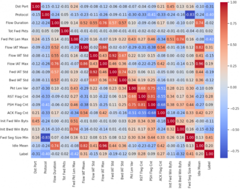
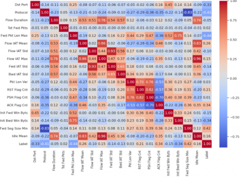
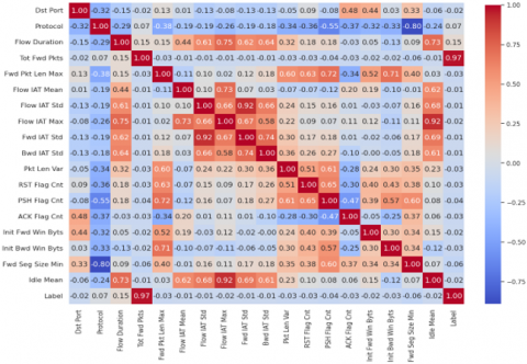
Subsequently, we applied the oversampling techniques SMOTE, ADASYN and BorderlineSMOTE to the unbalanced binary datasets. By splitting the data in this way, we enable resampling techniques to focus on the specific characteristics of each attack class, rather than aggregating them all into a single "Abnormal" class. This approach enables finer-grained management of class imbalance by recognizing the diversity of DDoS attacks and tailoring resampling techniques to each attack type. The aim is to generate synthetic data that faithfully captures the characteristics of each type of attack, thus improving the ability of models to effectively detect these specific attacks. To assess the quality of the synthetic data generated on these binary datasets, we first used the Kolmogorov-Smirnov test, then compared the correlation matrices between the real and synthetic data. Subsequently, we evaluated the effectiveness of the LGBM and XGBoost models before and after synthesizing using the macro_f1-score and AUC_ROC metrics, and finally carried out tests on the learning and synthesizing times to assess the operational efficiency of the synthetic generation methods.
One of the main objectives of our approach is to minimize the number of false positives, which are a major source of false alarms for intrusion detection systems. The resampling techniques used to balance the datasets have improved the sensitivity of the models to DDoS attack detection, while reducing the number of false positives and thus lowering classification errors. Furthermore, by considering execution time in our method, we strive to provide efficient and responsive solutions for DDoS attack detection, ensuring that IDSs can identify threats more quickly, thereby minimizing response time.
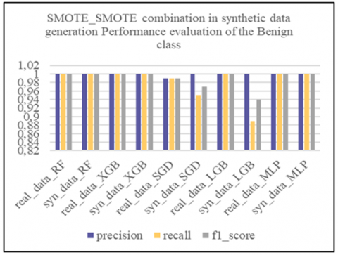
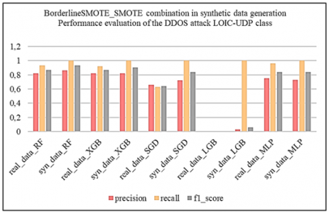
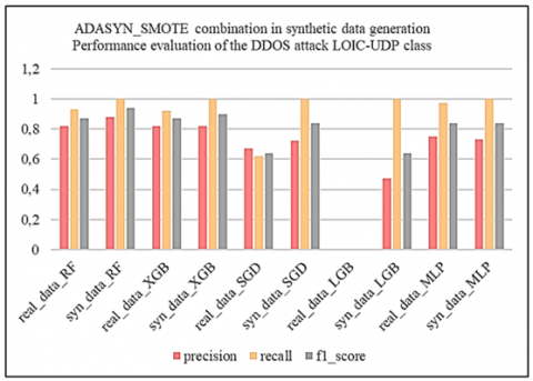
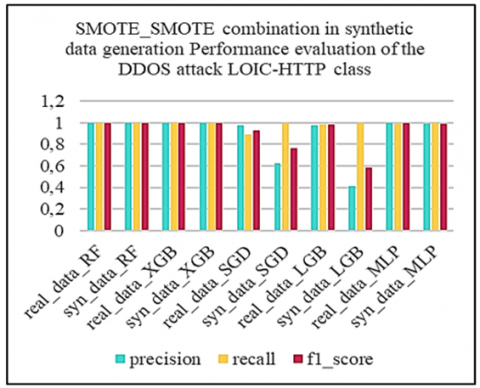
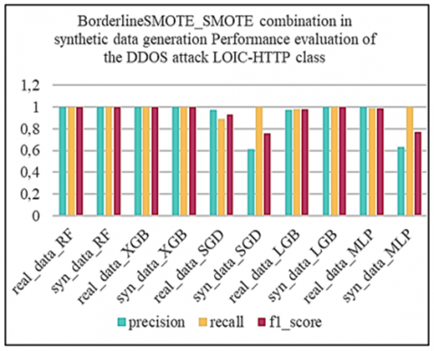
Subsequently, from the fusion of the generated synthetic binary sets with the remaining balanced binary set, we constructed the global synthetic multi-class artificially balanced dataset. This global synthetic dataset was evaluated by comparing the performance of machine learning models including Random Forest (RF), eXtreme Gradient Boosting, XGBoost (XGB), Stochastic Gradient Descent (SGD), Light Gradient Boosting Machine (LGBM) and Multilayer Perceptron (MLP). These models were first trained on real data, then re-trained on synthetic data before being evaluated with the application of real test data. Performance tests on the models revealed that the XGB model, with the “ADASYN, SMOTE” combination corresponding to the resampling techniques respectively applied to the DDoS attack classes [LOIC-HTTP, LOIC-UDP], performed best against the defined criteria, namely accuracy, precision, recall, f1_score, false positive rate (FPR), and learning and prediction times for operational efficiency.
By integrating these different approaches, our method provides an effective solution to the specific problems encountered by IDSs in detecting DDoS attacks.
The rest of the document is organized as follows: Section II discusses related work, while Section III presents the fundamental concepts incorporated into our solution. Section IV presents the CSE-CICIDS2018 dataset and in more detail the part of this dataset related to DDOS attacks. Section V details our approach. Section VI describes the implementation of our method, presents the results obtained, and discusses their effectiveness. Finally, Section VII concludes the paper with a look at future work.
Network security faces malicious attacks from various sources, and intrusion detection systems are essential for ensuring security. These systems are a significant research focus within network security, drawing numerous researchers dedicated to enhancing and optimizing the technology. Recently, numerous intrusion detection and prevention techniques leveraging machine learning algorithms have been proposed to enhance attack detection. In this section, we review some relevant prior work that has presented methods to improve the performance of IDS. They have focused on data pre-processing, feature selection, class imbalance resolution using oversampling and/or under sampling methods and classifier optimization.
Liu et al. [3] present in their research work a network intrusion detection system based on two main components. First, the adaptive synthetic oversampling technology (ADASYN) is employed to increase minority samples, addressing the issue of low detection rates for minority attacks caused by imbalanced training data. Second, the LightGBM model is integrated to reduce the system's temporal complexity while maintaining detection accuracy. Experiments included ADASYN and other resampling techniques, such as random downsampling (RD), Near-miss, condensed nearest neighbor (CNN), neighborhood cleaning rule (NCL), cluster centroids (CC), random oversampling (RO), and synthetic minority oversampling technique (SMOTE) for comparison. Additionally, various machine learning algorithms were explored, including DT, LR, NBM, KNN, ANN, SVM, RF, GBDT, Adaboost, and LightGBM. Evaluation metrics comprised accuracy, precision, recall, false alarm rate, training and detection times, as well as Friedman and Nemenyi post-hoc tests. Tests conducted on the NSL-KDD, UNSW-NB15, and CICIDS2017 datasets demonstrated an improved detection rate for minority samples after applying ADASYN oversampling, along with an increase in overall accuracy rates. The intrusion detection algorithm based on ADASYN and LightGBM achieved accuracies of 92.57%, 89.56%, and 99.91% for the three datasets, respectively, and showed reductions in the processing time of learning and detection phases as well as decreased false alarm rates.
The study described in Latif et al. [4] was carried out in several successive stages, where the results of each phase represent the combinations that generate the best performance for that stage. The resulting combinations were considered as the input parameters for the next phase. The researchers began their analysis by exploring different pairings of machine learning algorithms in conjunction with various feature scaling techniques. These combinations were then integrated with feature reduction methods, and finally with oversampling approaches. The objective was to determine the most optimal combination of these techniques for intrusion detection systems. The study examined various machine learning algorithms including Decision Tree, Support Vector Machine, Random Forest, Naïve Bayes, Neural Network, and AdaBoost. Techniques for scaling features involved normalization and standardization. Methods for reducing features incorporated the use of a low variance filter, high correlation filter, random forest, and incremental PCA. Various oversampling methods, such as SMOTE, Borderline-SMOTE and ADASYN, were also applied. The NSL-KDD dataset was used as a reference, with performance metrics including accuracy, precision, recall, and learning and prediction times. Among the combinations evaluated, the KNN + Normalization + Correlation filter + Borderline SMOTE algorithm was singled out for its higher performance compared with the other combinations of techniques studied.
In the study by Chen et al. [5], the assessment of intrusion detection is based on the use of the CICIDS 2017 dataset. Features with a correlation coefficient greater than 0.95 were excluded during the pre-processing phase. To select the machine learning algorithm to be used to train the classification model for intrusion detection, the authors carried out a cross-validation comparison of the performance of Random Forest, Naive Bayesian, Logistic Regression, KNN and CART. The results of this evaluation indicate that Random Forest performs best. The study then integrated the Random Forest algorithm with three distinct sampling techniques-Random Under-Sampling, SMOTE, and ADASYN. Through a comparative analysis aimed at enhancing precision, recall, F1 scores, and AUC values, it was found that combining ADASYN with Random Forest particularly excelled in addressing class imbalance issues. This method also facilitated precise classification and efficient detection of network attack behaviors.
To resolve the challenge of class imbalance within the data and improve network intrusion detection, Pan and Xie [6] exploited the KDD CUP99 dataset in their study. To mitigate the redundancy of sample features in this dataset, the authors implemented the PCA algorithm. To alleviate the class imbalance, they adopted ADASYN. Subsequently, the original datasets and those treated by PCA + ADASYN were used to conduct experiments with Random Forest (RF), Support Vector Machine (SVM), and XGBoost. To evaluate the effectiveness of the models using this approach, the F1_score and FPR metrics were used. The results indicated that the PCA + ADASYN + XGBoost method performed best.
The study conducted by Li et al. [7] exploited the UNSW-NB15 network traffic dataset. Due to the uneven distribution of different attacks in this dataset, the authors consolidated the anomalous behaviors into a single category, thus becoming the majority category. The study proposes a two-pronged approach: using the Adasyn oversampling method to resolve the imbalance between normal and abnormal data, and adopting the ID3 decision tree algorithm for categorizing traffic into two types to detect network intrusions. To assess the model's effectiveness, this approach was benchmarked against other machine learning methods including K-nearest neighbor (KNN), logistic regression, support vector machine (SVC) classifier, random forest, adaboost, decision tree (using the ID3 algorithm), and a hybrid approach (ADASYN + ID3). The evaluation metrics focused on accuracy, precision, recall, and the false alarm rate. Findings reveal that the hybrid model combining ADASYN with the ID3 decision tree, as suggested in this study, achieves higher accuracy and a reduced false alarm rate, proving effective for intrusion detection tasks.
Sun et al. [8] presented an approach to solve the problem of multiple classification of network intrusions, with a study conducted on the CIC-IDS2017 dataset. To overcome data imbalance, the researchers designed a resampling approach that involves random sampling and Borderline SMOTE oversampling to balance the data. To select features, they computed the rate of information gain for each feature and each attack category in the balanced data set. Subsequently, experiments were conducted with three machine learning algorithms (KNN, DT, RF), trained on six feature sets, to obtain optimal feature selection and the best machine learning method.
This paper Wu et al. [9] addresses data imbalance by proposing a network intrusion detection algorithm that uses an improved random forest in conjunction with the SMOTE upsampling technique. In the first phase, authors introduce a combined sampling approach that associates K-means algorithm and SMOTE algorithm. This method aims to decrease number of outliers, enrich characteristics of minority samples and augment number of samples in this class. Preliminary prediction results are then obtained using an improved random forest. The decision tree with the highest classification performance within the random forest framework is selected for similarity computation in the next step. Following this, a similarity matrix for network attacks is utilized to refine the prediction results during the voting process, through an analysis of the attack types. Finally, the improved random forest model and other machine learning algorithms, including KNN, SVM and RF, are trained on the NSL-KDD dataset. The proposed model displays outstanding performance, attaining a classification accuracy of 99.72% on the training set and 78.47% on the test set.
In this study, Talukdera et al. [10] present a hybrid approach incorporating suitable pre-processing, including missing value handling, feature normalization and label encoding to prepare datasets. They also apply the SMOTE technique to balance the data and use XGBoost for feature selection. Different ML and DL algorithms, including RF, DT, KNN, MLP, CNN and ANN, are used to evaluate effectiveness of the method in detecting network intrusions. Tests are performed using the datasets, KDDCUP'99 and CIC-MalMem-2022. Various performance measures, including accuracy, precision, recall, F1 score, AUC score, ROC curve, MAE, MSE and RMSE, are used to evaluate the algorithms in both binary and multi-class attack contexts. The findings indicate that the RF algorithm particularly excels, achieving the highest accuracy rate of 99.99% on the KDDCUP'99 dataset and 100% on the CIC-MalMem-2022 dataset, without exhibiting overfitting and Type-1 or Type-2 errors.
Alshamy et al. [11] present in their study an IDS model (IDS-SMOTE-RF) that exploits the SMOTE oversampling technique to solve the class imbalance problem and uses the Random Forest algorithm to detect various types of attacks. The model was formed and tested using the NSL-KDD dataset. A comparative analysis was conducted between the IDS-SMOTE-RF model and other classifiers, including Adaboost (AB), Logistic Regression (LR) and Support Vector Machine (SVM), focusing on measurements like accuracy, precision, recall, the F1 score, and the time required to process binary and multi-class classifications. The experimental results revealed that the IDS-SMOTE-RF model achieved a high accuracy of 99.89% in binary classification and 99.88% in multi-class classification, thereby proving to be the most efficient in terms of prediction time.
Generally, within the domain of intrusion detection systems, research goals are centered on refining machine learning algorithms and enhancing overall dataset learning metrics, including model accuracy, detection rate, reduction in false alarm rates, and minimizing learning and prediction times. Optimization methods include data preprocessing, feature selection, and/or reducing data dimensionality to boost model efficacy and decrease the consumption of computing resources. In addition, solving the imbalance of sample classes in datasets is also an important area of research. In this area of IDS, researchers can still bring suitable refinements to achieve better detection outcomes.
In this section, we will look at the technologies embedded in the solution we propose. We will begin with a detailed explanation of the approaches used for feature selection, including the correlation matrix and mutual information. The function of the XGBoost classifier will be explained in the last part of this section. Next, we will discuss oversampling methods such as SMOTE, Adasyn and BorderlineSMOTE, and then offer an overview of the machine learning models we have experienced.
3.1 Feature selection techniques
3.1.1 Correlation matrix
Feature selection in machine learning is an essential step aimed at reducing data dimensionality and enhancing model accuracy and efficiency. The correlation matrix, a statistical tool, identifies the features with the highest correlations in a dataset. Features with high correlation are often redundant and do not contribute to the model's predictive power. Eliminating these features can lead to better model performance.
In Data Science, the correlation matrix helps to quantify the relationships between variables, measuring the strength and direction of these links. It is represented by a table displaying correlation coefficients between variables. Each variable appears both in row and column, with the corresponding cell in the matrix containing the correlation coefficient for each pair of variables. The correlation coefficient varies between -1 and +1, with -1 representing a perfect negative correlation, +1 a perfect positive correlation, and 0 indicating no correlation between the variables. Coefficients reveal the nature of the relationship between variables, clarifying dependencies. Variables that tend to increase or decrease together have high positive correlation coefficients, while variables that tend to move in opposite directions exhibit high negative correlation coefficients [12]. This matrix is a powerful tool to determine which variables are significantly related or poorly correlated or not correlated at all, contributing to fact-based predictions and judgments [12]
The following formula calculates the correlation coefficient between two variables [12]:
$r=\frac{\left(n \sum X Y-\sum X \sum Y\right)}{\sqrt{\left(n \sum X^2-\left(\sum X\right)^2\right)\left(n \sum Y^2-\left(\sum Y\right)^2\right)}}$ (1)
where,
r: correlation coefficient,
n: number of observations,
$\sum X Y$: sum of the product of each pair of corresponding observations of the two variables,
$\sum X$: sum of observations of the first variable,
$\sum Y$: sum of the observations of the second variable,
$\sum X^2$: sum of the squares of the observations of the first variable,
$\sum Y^2$: sum of the squares of the observations of the second variable.
Although the correlation matrix is useful for feature selection in machine learning, it is recommended to use it judiciously alongside other feature selection methods to prevent over-fitting or under-fitting the model. Leveraging the correlation matrix, machine learning algorithms can identify the most relevant features, thereby enhancing their predictive power.
3.1.2 Mutual information
Mutual information quantifies the dependence between two random variables. High mutual information indicates strong dependence, while low mutual information suggests independence between the variables. The mutual information between two random variables X and Y is mathematically defined as follows:
$I(X ; Y)=\sum_{x \in X} \sum_{y \in Y} P(x, y) * \log \left(\frac{P(x, y)}{P(x) * P(y)}\right)$ (2)
where,
$P(x, y)$ is the joint probability of $X=x$ and $Y=y$
$P(x)$ and $P(y)$ are the marginal probabilities of $X$ and $Y$
$I(X ; Y)=0$ if and only if x and y are independent
$I(X ; Y)$ is symmetric, i.e. $I(X ; Y)=I(Y ; X)$
In machine learning, it is often employed to assess relationships between features in a dataset and is useful for feature selection. It can also be used to evaluate the connection between each feature and the target variable (label), allowing the retention of the most informative features while reducing redundancy during dimensionality reduction. Features are ranked based on their mutual information with the target variable, with those having the highest mutual information being retained [13]. This streamlines the decision-making process and improves accuracy by reducing noise and eliminating unnecessary complexity [14]. In the context of clustering, mutual information can be used to measure the similarity between two clusters, notably in algorithms such as hierarchical agglomeration methods. Although sensitive to non-linearity and capable of detecting dependencies not captured by linear measures such as correlation, mutual information can be influenced by the granularity of the data, requiring precautions when using it [14].
In summary, mutual information is emerging as a powerful measure for quantifying the dependency between two variables, making it valuable in numerous machine learning applications, such as feature selection and dimensionality reduction.
3.2 Oversampling techniques
3.2.1 Smote
SMOTE (Synthetic Minority Over-Sampling Technique) is an over-sampling technique developed to rebalance training sets with an under-representation of the minority class. The aim is to strengthen the minority class by generating synthetic examples. Instead of simply duplicating existing instances of the minority class, SMOTE introduces synthetic examples by performing a linear interpolation between several instances of this class located in a defined neighborhood, using Euclidean distance and k-NN (k Nearest Neighbors) [15]. The process of creating synthetic instances first involves defining the total number of oversamples N, which is the number of instances that will need to be generated to obtain a balanced distribution of classes [16]. Next, an iterative process consisting of several steps is implemented. SMOTE randomly selects an instance of the minority class and uses Euclidean distance to identify the k nearest neighbors of the same class. The parameter k is a user-defined number, usually k=5 (default). The new synthetic examples are generated by linearly interpolating between the selected instance and some of its neighbors, adjusting the feature values according to the differences between the selected instance and its neighbors. The complete process is shown below:
Let $x_i$ be an instance of the minority class, and $x_{i 1}$, $x_{i 2}, \ldots, x_{i K}$, the $K$ nearest neighbours of $x_i$ in the training set.
1) Random selection of an instance of the minority class
a. Random selection of an instance of the minority class $x_i$
2) Calculation of new synthetic instances
a. For each instance $x_{i j}$ among the $K$ nearest neighbours, we calculate the difference
$\operatorname{diff}=x_{i j}-x_i$
b. For each instance $x_{i j}$, a random number $u$ is generated between 0 and 1
c. For each instance $x_{i j}$, the new synthetic instance is calculated using the following interpolation formula: $x_{\text {synij }}=x_i+u * \operatorname{diff}$
d. These steps are repeated to create $N$ new synthetic instances.
e. The set of new synthetic instances created is noted $\left\{x_{\text {syni } 1}, x_{\text {syni } 2}, \ldots, x_{\text {syniN}}\right\}$.
f. Repeating these steps $N$ times to select $N$ instances of the minority class and create $N \times K$ new synthetic instances.
3) Applying the oversampling method
a. The synthetic instances $x_{\text {syni } 1}, x_{\text {syni } 2}, \ldots, x_{\text {syniN }}$ are added to the training set.
This process aims to introduce variability while avoiding simple replication of existing instances. The use of Euclidean distance and k-NN ensures that synthetic instances are relevant to the local distribution of the data. In general, SMOTE focuses on the feature space instead of the data space [16]. This means that the specific features defining a class are taken into account when generating synthetic examples, thus preserving the local structure of the minority class. By exploiting the relationships between sample features, SMOTE improves the ability of models to deal with class imbalance.
Note that SMOTE is only applicable to continuous data. An adapted version, SMOTENC (SMOTE Nominal Continuous) [17], exists for categorical data. Despite its advantages, SMOTE has some weaknesses, notably that it does not take into account neighboring examples of the majority class. In fact, the synthetic observations created for the minority class may overlap with instances of this class. In addition, the excessive generation of synthetic observations may introduce additional noise into the dataset, potentially biasing the model [17].
The creation of synthetic instances has led to an in-depth study of the theoretical relationships between original and synthetic instances, taking into account aspects such as data dimensionality, variance, correlation in data and feature space, and the distribution between training and test instances [16]. In summary, SMOTE provides an efficient method for oversampling the minority class, generating relevant synthetic examples based on relationships in feature space, thus helping to maintain minority class structure and diversity, improve dataset balance and enhance model performance in imbalanced class scenarios.
3.2.2 Borderline-SMOTE
Borderline-SMOTE is a variation of the original SMOTE, an improvement on the algorithm [4], designed to better handle examples located at the border between majority and minority classes in an unbalanced dataset. Borderline-SMOTE is based on the idea that examples located at the border between classes are more relevant for oversampling. It uses the ratio between the majority and minority examples in the neighborhood of each instance to identify the examples belonging to the borderline. Borderline-SMOTE classifies examples into three categories: "Safe", "Danger" and "Noise". "Safe" examples are those where the majority of neighbors appertain to the same minority class, while "Dangerous" examples are on the borderline with a more balanced proportion of neighbors from both classes. Noise" examples are characterized by neighbors all belonging to the majority class [8, 16]. Only the "Dangerous" examples are selected for oversampling [16]. The aim is to improve the distribution of example categories without generating noise from examples that are clearly in the majority. Borderline-SMOTE uses the SMOTE algorithm to generate new synthetic examples. It selects a "Dangerous" example and calculates its k nearest neighbors. It then synthesizes new examples by performing a weighted interpolation between the original example and its neighbors.
3.2.3 Adasyn
ADASYN (Adaptive Synthetic Sampling) is an adaptive synthetic sampling technique designed to solve the problem of class imbalance in data sets. The technique is based on the assumption that not all examples in the minority class are equally difficult to learn. Some minority examples are considered more difficult to learn than others based on the proportion of the majority class in their vicinity [16]. ADASYN assigns different weights to the examples in the minority class based on their learning difficulty level [5, 16]. Minority examples considered more difficult to learn receive a higher weighting. Unlike SMOTE, which generates the same number of synthetic samples for each minority example, ADASYN is density adaptive, generating more synthetic samples in areas where the density of minority instances is low. In addition, SMOTE uses a fixed factor to determine the number of synthetic samples, whereas ADASYN adjusts the number of synthetic samples based on the estimated learning difficulty, considering the ratio of majority class neighbors to the total number of neighbors.
The minority examples that are more difficult to learn are associated with a higher production of synthetic samples, while those considered easier require fewer synthetic samples. The ADASYN algorithm aims to achieve a relative balance of classes by generating synthetic examples where this is deemed more necessary, depending on the estimated level of learning difficulty.
The ADASYN algorithm can be detailed as follows [3, 7]:
Input:
D: initial training dataset with $m$ instances.
$\left\{x_i, y_i\right\}$ where $x_i$ is an instance in the feature space $X$ and $y_i$ is the identity label of the class associated with $x_i$
$m_s$: number of instances of the minority class.
$m_l$: number of examples of the majority class.
$k$: number of nearest neighbors to consider.
dth: threshold value for the maximum degree of imbalance between classes.
Output:
$D^{\prime}$: oversampled data set.
1) Calculation of the degree of imbalance between classes, imbalance $=m_s / m_l$
2) Check whether the degree of imbalance is less than the dth threshold. If true, then:
a. Calculate the total number of synthetic samples to generate: $G=\left(m_l-m_s\right)*$ imbalance
b. For each minority example $x_i$.
1) Calculate the learning difficulty level which is the ratio of majority class neighbors among the k nearest neighbours of $x_i$, difficulty $y_i=$ ((number of neighbors belonging to the majority class among the k nearest neighbours of $\left.x_i\right) / \mathrm{k}$).
2) Difficulty level normalization:
$\text { normalized_difficulty }_i=\frac{\text { difficulty }_i}{\sum_{i=1}^{m_s} \text { difficulty }_i}$
3) Adjustment of the difficulty level:
adjusted_difficultyi = normalized_difficultyi × G
4) Calculation of the number of synthetic samples to generate:
$\text { num_synthetic }_i=\text { rounded }\left(\text { adjusted_difficulty }_i\right)$
5) Generation of synthetic samples:
Steps 1 to 5 of point b are repeated until the desired equilibrium is reached or until a predefined stopping criterion is satisfied.
ADASYN is a flexible approach that adapts the generation of synthetic samples according to the complexity of the minority examples, providing an adaptive solution to the class imbalance problem.
3.3 Machine learning algorithms
In our research, we selected several machine learning algorithms based on their specific characteristics and adaptability to the CICIDS2018 DDOS attack dataset. Since DDoS attacks generally involve a large volume of malicious network traffic, we deemed it essential to use models adept at efficiently processing vast amounts of data and identifying anomalous patterns. The RF model was chosen for its capacity to manage complex data sets with interdependent explanatory variables, while offering good robustness to outliers and over-fitting. We also favored the use of XGB, due to its proficiency in handling large datasets with great efficiency in terms of speed and performance. On the other hand, SGD seemed the obvious choice, given its efficiency in learning from massive data and its ability to converge rapidly to optimal solutions, making it well suited to our large dataset. For its part, the LGB was chosen for its speed of execution and its ability to handle class imbalance. These two criteria are, in fact, an eminently important aspect for our dataset, where DDoS attacks represent a minority class. Finally, MLP was selected for its power to identify complex patterns in the data due to its multilayer neural network structure, which is beneficial for detecting subtle patterns present in our CICIDS2018 DDOS attack dataset.
In sum, by exploiting these algorithms in our study, we were able to experiment their respective strengths to enhance the performance of our DDoS attack detection model on this specific dataset. A detailed description of these algorithms is given below:
3.3.1 Random forest
Random Forest is a powerful supervised classification method [18]. It is distinguished by its use of subsets of the original dataset to make predictions. During training, it constructs many individual decision trees with different sets of observations, and the predictions from these trees are then combined, typically using majority voting, to produce the final prediction [1, 19]. This approach, known as the ensemble technique, solves the over-fitting problem [20] by relying on the majority ranking of all tree results.
Random forests are versatile and can be applied to both classification and regression tasks. For classification, a random forest gathers a class vote from each tree and then determines the final classification based on the majority vote. For regression, the predictions from each tree for a target value are averaged.
The goal of minimizing the correlation between trees in random forests is to decrease the model's variance by encouraging diversity among the trees. Each tree is built using a random subset of the training data and random subsets of features, leading to the creation of distinct trees [21]. This diversity ensures that each tree can make unique prediction errors since they are trained on different data samples. By combining these predictions, either through averaging or a majority vote (for classification), the overall model variance is reduced [1]. This approach prevents over-fitting, as the errors made by one tree are balanced out by the accurate predictions of others [22]. When the predictions of trees show a high correlation, this indicates that these trees generally make similar errors. In such situations, the application of averaging or voting would not lead to a significant improvement in performance [1]. By emphasizing diversity and reducing correlation, Random Forest increases the stability of predictions, improving the generalization of the model to unknown data. Hence, the results become more reliable, resulting in improved predictive performance.
An additional advantage of this algorithm is its ability to perform feature selection, measuring the importance of each variable at each division of each tree. This importance is calculated as a function of the improvement in the division criterion, pondered by the likelihood of reaching the corresponding node [20, 21].
Random Forest is robust and efficient for classification, making it an appropriate choice for detecting abnormal patterns of network activity. It excels at handling large amounts of data and is capable of handling complex features.
3.3.2 Xgboost
XGBoost (Extreme Gradient Boosting) is one of the most popular and efficient machine learning algorithms, frequently employed for regression and classification fields. Its high predictive performance and remarkable efficiency have increased its popularity in recent years [23]. XGBoost outperforms the gradient-based decision tree (GBDT) algorithm with regard generalization, scalability and to computational speed [24].
XGBoost, a technique for ensemble learning, enhances predictive accuracy by optimizing a regularized loss function through the combination of multiple decision trees. The algorithm employs a reinforcement procedure that involves the successively training of numerous decision trees. During each iteration, an additional tree is introduced to correct the residual mistakes from the preceding trees. The contributions of these trees to form the ultimate prediction are then weighted according on their individual effectiveness [1].
Consider a training dataset composed of feature-label pairs $\left\{\left(x_i, y_i\right)\right\}_{i=1}^n$, where xi denotes the set of features for the ith example and yi represents its associated real class label.
The primary goal of XGBoost is to construct a predictive model $F(x)$ that minimizes a regularized loss function $L\left(y_i, F\left(x_i\right)\right)$ by accurately predicting the labels yi. The optimization goal of XGBoost can be formulated as follows [1]:
$L(\theta)=\sum_{i=1}^n L\left(y_i, F\left(x_i\right)\right)+\sum_{j=1}^T \Omega\left(f_j\right)$ (3)
The function $L\left(y_i, F\left(x_i\right)\right)$ serves as a metric for quantifying the divergence between the model's prediction $F\left(x_i\right)$ and the actual label yi. Among the frequently employed convex loss functions are the logarithmic, square, and exponential loss functions. The variable $T$ signifies the cumulative count of trees within the ensemble, with $f_j(x)$ denoting the function represented by the jth tree in the ensemble. The term $\Omega\left(f_j\right)$ acts as a regularization component, imposing a penalty on the intricacy of the trees to prevent the model from overfitting. This term is formulated as follows [1]:
$\Omega\left(f_j\right)=\gamma T_j+\frac{1}{2} \lambda \sum_{k=1}^L w_{j k}^2$ (4)
The parameters $\gamma$ and $\lambda$ are utilized to modulate the intensity of the regularization process. Here, $T_j$ represents the total count of leaves within a tree, $L$ denotes the number of nodes in tree $f_j$ and $w_{j k}$ signifies the weight associated with the $k$ th node in tree $f_j$. The initial component of the regularization function, $\gamma$ $T_j$, imposes a penalty that scales with the total number of leaves in the tree; the more numerous the leaves, the greater the penalty incurred. The second component, $\frac{1}{2} \lambda \sum_{k=1}^L w_{j k}^2$ within the XGBoost objective function, governs the extent to which the model is penalized for assigning higher weights to the leaves. As $\lambda$ increases, the algorithm tends to favor lower leaf weights, thereby promoting the development of more parsimonious trees. This regularization strategy serves to mitigate overfitting by curbing the propensity of overly intricate trees to model the noise present in the training data. The values for $\lambda$ and $\omega$ are typically determined through empirical means [25].
To reduce the loss function, the predictions $F(x)$ are updated by incorporating the predictions from each individual tree weighted by its respective learning coefficient $\eta$ [1]:
$F_t(x)=F_{t-1}(x)+\eta \sum_{j=1}^J f_j(x)$ (5)
The learning rate $\eta$ plays an important role as a hyperparameter, regulating the magnitude of the update. By employing the boosting approach, XGBoost constructs each tree with the objective of rectifying the residual errors from the preceding model. This iterative process enables the algorithm to gradually adapt to the residual errors as additional trees are introduced.
XGBoost offers the advantage of automatically generating assessments of feature importance from a trained predictive model. The importance of features is determined by examining their contribution to the building of the boosted decision trees, which reflects their relative significance within the model. The assessment of importance relies on the enhancement in the performance measure for each attribute-sharing point in a tree, with weighting by the number of instances linked to the node. Ultimately, XGBoost computes the average of these importance scores across all the decision trees in the model, delivering a comprehensive estimate of the importance of each feature. This process makes it possible to rank characteristics according to their contribution to performance, offering insights into the most influential variables in the model [26].
XGBoost offers high accuracy and good generalization. Its ability to handle unbalanced datasets can be useful in the context of DDoS attack detection, where malicious activity may be rare compared to normal traffic.
3.3.3 Stochastic gradient descent
Stochastic Gradient Descent (SGD) is a technique of iterative optimization that is extensively embraced in the realm of machine learning, particularly for the training of neural network models. This approach is applied to unconstrained optimization problems [27]. Basically, SGD is used to iteratively adjust the parameters of a model to minimize a cost function [28]. This function evaluates the discrepancy between the predictions made by the model and the true values, and is central to the learning process.
SGD is a derivative of classical gradient descent, and aims to update model parameters iteratively and incrementally, using mini-batches of data, representing a change from classical gradient descent which exploits the full dataset at each iteration [28]. This sequential approach enables faster training, which is particularly beneficial for large datasets.
Its efficiency stems from its ability to process data in small, bite-sized chunks, which significantly reduces memory requirements, making SGD ideal for large datasets. In addition, SGD tends to converge faster than its conventional counterpart, particularly in high-dimensional parameter spaces. However, this rapid convergence is accompanied by inherent variability due to stochastic sampling, making the process sometimes noisy. Furthermore, SGD requires careful management of the hyperparameters, in particular the choice of the learning rate (η). Inadequate selection of this value can compromise convergence, leading to either slow convergence or divergence. Thus, judicious adjustment of the parameters becomes a crucial step in guaranteeing fast and stable convergence.
The mathematical formulation of stochastic gradient descent presented in the literature [27, 28] is as follows:
Given a training dataset consisting of $\left(x_1, y_1\right), \ldots,\left(x_n, y_n\right)$, where $n$ is the number of examples, $x_i \in \boldsymbol{R}^m$ represents the features of the $i$ th example and $y_i \in \mathcal{R}$ is the target label associated with this example.
The goal is to learn the linear score function $f(x)=w^T x+$ $b$, with the model parameters, $w \in \boldsymbol{R}^m$ the weight vector and, $b \in \boldsymbol{R}$ the intercept.
The learning objective is to determine the optimal values of the model parameters $w$ and $b$ that minimize the regularized learning error $E(w, b)$ given by:
$E(w, b)=\frac{1}{n} \sum_{i=1}^n L\left(y_i, f\left(x_i\right)\right)+\alpha R(w)$ (6)
where, $L(y, f(x))$ denotes a loss function assessing model fit. It evaluates how closely the prediction $f(x)$ matches the true target $y . R(w)$ a regularization term that penalizes the model's intricacy. This term helps prevent over-fitting by restricting the values of model parameters. a represents a positive hyperparameter that governs the degree of regularization.
The SGD algorithm uses optimization techniques such as gradient descent to adjust model parameters iteratively until convergence. It progresses through the training data, and for each entry, it updates the model parameters following the specified update rule below:
$w \leftarrow w-\eta\left[\alpha \frac{\partial R(w)}{\partial w}+\frac{\partial L\left(w^T x_i+b, y_i\right)}{\partial w}\right]$ (7)
In this context, $\eta$ represents the learning rate, determining the step size of the updates in the parameter space. The intercept $b$ is updated similarly, yet it is not subject to regularization.
The convergence of SGD may occur more quickly, yet the noise introduced by randomly choicing samples may render the algorithm less stabe compared to classical gradient descent. However, many techniques and variants have been developed to mitigate these problems and improve the stability and efficiency of training, making it an essential tool in modern machine learning.
Stochastic Gradient Descent (SGD) can be adopted as a model for detecting DDoS attacks, due to its ability to efficiently process large datasets. The stochastic nature of SGD, using mini-samples in an iterative fashion, enables rapid training on real-time data streams, a crucial feature for the detection of constantly evolving attacks. SGD can be a relevant choice for intrusion detection in a network security context.
3.3.4 LightGBM
Light Gradient Boosting Machine, or LightGBM, is a machine learning algorithm developed by Microsoft, based on the gradient boosting technique. Its distinction lies in its ability to efficiently manage large datasets, offering fast and parallel performance [29]. As a boosting model, LightGBM combines several weak models, often shallow decision trees, in an assembly method to create a more powerful global model. Based on the gradient reinforcement algorithm, LightGBM successively trains models, focusing on examples that are poorly predicted by previous models, with each model aiming to rectify the mistakes of its predecessor. This algorithm is applied in a range of tasks including classification, regression and large-scale ranking, making it effective for solving a variety of problems in machine learning [29]. Three distinct methods bolster LightGBM's capabilities: Gradient-based One-Side Sampling (GOSS), Exclusive Feature Bundling (EFB), and the histogram-based approach for choosing features and identifying segmentation points [3, 30]. These techniques are seamlessly integrated into the overall decision tree building process when models are trained with LightGBM.
The Gradient-based One-Side Sampling (GOSS) algorithm is introduced in LightGBM with the goal of decreasing the number of samples at each iteration while emphasizing the training of samples that show weak predictive performance. During each iteration, LightGBM first calculates the gradients for all the instances in the dataset. The instances are then sorted according to the magnitude of their gradients. This separates the most informative instances from those that have less impact on the model. GOSS retains a large proportion of the instances with high gradients, thus preserving the most relevant information for learning [3]. Random sampling is carried out among the instances with lower gradients [3]. This reduces their number, while preserving a reasonable representation of these less informative examples. LightGBM then uses these sampled instances to update the model parameters using gradient descent. Updates are made incrementally and selectively, making it easier to learn difficult cases. By lowering the sample volume processed in each iteration, GOSS contributes to a reduction in computational load, which is particularly advantageous for handling massive datasets. It allows more focus to be placed on instances with poor prediction effects, helping to reinforce the learning of these difficult cases, improve model efficiency and achieve more accurate predictions.
EFB is a technique introduced in LightGBM for grouping features that are mutually exclusive. This method seeks to decrease the dimensionality of the feature space, which in turn enhances the efficiency of model training. LightGBM analyses the features in the dataset to identify those that are mutually exclusive, i.e. those that are never simultaneously active in the same decision tree. Features that are mutually exclusive are grouped into sets [3]. For example, if two features A and B are mutually exclusive, they will be grouped together in a set. For each set of mutually exclusive features identified, LightGBM creates a new aggregated feature that represents these combined features. This aggregation can take different forms, such as average, sum, or other statistical operations. When building decision trees, instead of using individual features, LightGBM uses the new aggregated features created by the mutually exclusive grouping. By diminishing the feature space dimensionality, EFB helps to speed up model training, while retaining essential information. Indeed, by grouping mutually exclusive features, EFB simplifies the structure of decision trees by lessening the number of nodes required to depict the relationships between features, which reduces the time needed to train the model [30]. The creation of new aggregated features additionally lessens the model's complexity. By diminishing the number of features employed in the model, EFB contributes to better memory management, which is particularly useful for massive datasets [30]. In summary, Exclusive Feature Bundling (EFB) in LightGBM provides an efficient way to manage mutually exclusive features by grouping them together, reducing model complexity and improving training efficiency [30].
LightGBM uses the histogram algorithm to select features and determine segmentation points when building each decision tree [31]. Instead of examining all unique feature values to identify the optimal segmentation point (which is costly in terms of computation time), LightGBM uses histograms to approximate the distribution of feature values. Histograms are constructed for each feature and are used to find optimal segmentation points more quickly. This approach considerably speeds up the construction of decision trees in LightGBM, making it an effective algorithm for large or high-dimensional datasets [31].
By combining these techniques, LightGBM manages to deliver high performance with increased computational efficiency, even in complex, high-volume data contexts, making it a popular choice for supervised learning on large amounts of data. For these reasons, it can be particularly well suited to the detection of DDoS attacks.
3.3.5 MLP (Multilayer Perceptron)
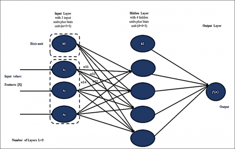
The Multi-Layer Perceptron (MLP) is an artificial neural network with a multi-layered architecture, including an input layer, hidden layers, and an output layer. It is commonly employed for various machine learning tasks, including classification and regression, due to its capability to model complex and non-linear relationships in data [32]. Figure 1 displays an MLP hidden layer with scalar output [33, 34].
The first layer of the MLP, called the input layer, receives the characteristics of the dataset, where each neuron represents an input characteristic. The total number of neurons in this layer is the total number of characteristics in the dataset [32, 35]. MLP includes one or more hidden layers located intermediate to the input and output layers, each made up of neurons. Each neuron in a hidden layer is connected to all neurons in the previous and next layers. It transforms the values of the previous layer by weighted linear summation, followed by a non-linear activation function. Within a hidden layer, neurons do not interact directly with each other, but indirectly through weighted connections, allowing the network to learn complex connections and representations in the data. The number of hidden layers and the number of neurons in each layer affects the complexity of the task [35]. The last layer, designated as the output layer, produces the model predictions using the information processed in the hidden layers. The output layer activation function depends on the type of problem to be solved, such as the sigmoid function for binary classification, the softmax function for multi-class classification, or no activation for regression.
The mathematical formulation of the MLP model is as follows:
Suppose we have an MLP with L layers, where layer 1 is composed of $n^{(l)}$ neurons. Let X be the input vector of dimension $\mathrm{d}, W^{(l)}$ the weight matrix of layer $1, b^{(l)}$ the bias vector of layer 1 , and $a^{(l)}$ the activation vector of layer 1.
Forward propagation through the network can be described as follows:
Figure 1. One hidden layer MLP
For hidden layer l:
$\begin{aligned} z^{(l)}= & W^{(l)} \cdot a^{(l-1)}+b^{(l)} \\ & a^{(l)}=\mathrm{f}\left(z^{(l)}\right)\end{aligned}$
where, $f$ is a non-linear activation function, such as the sigmoid function, the hyperbolic tangent (tanh), or the ReLU (Rectified Linear Unit) function.
For the last output layer L:
$\begin{gathered}z^{(L)}=W^{(L)} a^{(L-1)}+b^{(L)} \\ \hat{y}=\mathrm{f}\left(z^{(L)}\right)\end{gathered}$
where, $\hat{y}$ is the predicted output of the network, typically used for classification or regression, and $f$ is the activation function appropriate for the specific task.
The MLP assigns weights to each input feature, adjusted during training to optimize their value. The perceptron combines these weighted inputs through a summation function, while the neurons of the hidden layers apply activation functions to introduce nonlinearity, allowing the modeling of complex relationships. The information propagates through the network from the input layer to the output layer, generating predictions. For model learning, a loss function J is defined to measure the difference between model predictions and true labels. Examples of commonly used loss functions are mean squared error for regression and cross-entropy loss for classification. Next, backpropagation is used to adjust network weights and biases in order to minimize the loss function. Indeed, once the network output has been calculated and the loss function evaluated, error backpropagation is used to calculate the gradients of the loss function with respect to the network weights and biases. These gradients are then used to update the network weights and biases using an optimization algorithm such as stochastic gradient descent (SGD) or the gradient descent with momentum algorithm [34, 36].
MLPs are capable of capturing complex nonlinear relationships in data. They can be used to model sophisticated network activity patterns, which can be important for detecting DDoS attacks. However, MLPs have the following disadvantages: MLPs with hidden layers have a non-convex loss function where more than one local minimum exists. Consequently, different random weight initializations can lead to different validation accuracy. In addition, MLP requires the setting of a number of hyperparameters such as the number of hidden neurons, layers and iterations, and is sensitive to feature scaling.
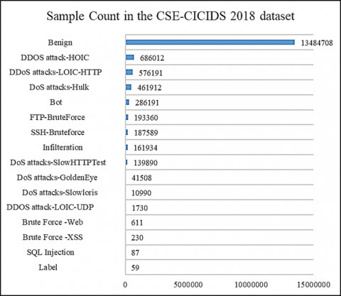
The CSE-CIC-IDS2018 (Canadian Institute for Cybersecurity Intrusion Detection System 2018) dataset is a widely used resource for intrusion detection system research and development. It was produced by the Canadian Institute for Cybersecurity (CIC) in collaboration with the Communications Security Establishment (CSE) [37]. The main objective is to create a comprehensive reference database for intrusion detection systems based on anomalies. This dataset was designed to simulate a realistic network environment by integrating normal network traffic data as well as data representing various potential attacks. The foundation of this project is built on creating user profiles that encapsulate abstracted event and behavior observed across the network, combining these profiles to create diverse datasets. The data comes from various sources, including attack simulations and real network traffic captures. This ensures a variety of representative instances of the scenarios encountered in the real world. The behaviors and patterns observed in the data are representative of real activities on today's computer networks. Collected over a 10-day period, from February 14 to March 2, 2018, the dataset captures seven distinct types of attack scenarios, including brute force, botnets, DoS/DDoS, web-based attacks, and network infiltrations. It comprises data from network traffic captures, system logs for each machine, and 80 different attributes extracted from the traffic via CICFlowMeter-V3. These features include information such as IP addresses, ports, protocols, durations, packet size, TCP flags, and other data related to network packets. Each record in the dataset is labeled as normal or malicious, facilitating the use of supervised learning techniques for attack detection. This labeling enables researchers to train models that can accurately differentiate benign from malicious traffic. The data is usually provided as CSV files, making it easy to use with various data analysis and machine learning tools. This is a large data set, with a large number of instances, providing sufficient scope for training machine learning models. The dataset, downloaded from Kaggle, has 16,233,002 examples and 80 features, with variations in the availability of certain features depending on the registration dates. The diversity of this data makes it a valuable resource for network activity analysis, especially in the detection of attacks. Figure 2 presents the breakdown of instances in the CICIDS 2018 dataset, downloaded from Kaggle.
Figure 2. The instances breakdown of the CICIDS 2018 dataset
In sum, with over 16 million examples and 80 features extracted from traffic, the CICIDS2018 dataset offers a wealth of data essential for machine learning model entrainment. Consequently, the diversity of instances representative of scenarios encountered in the real world ensures that models are exposed to a wide range of situations, contributing to their generalization and robustness. Researchers and practitioners use the CSE-CICIDS2018 dataset to evaluate the performance of their IDSs, analyze attack trends, and develop more robust intrusion detection models. As a result, the size of the dataset, comprising millions of instances, provides a solid basis for assessing intrusion detection systems, allowing thorough analysis for the test of algorithms performances.
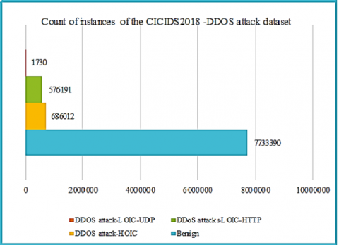
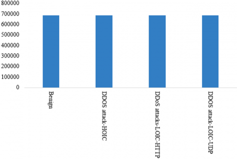
In our approach, we focused on DDoS attacks in the CSE-CIC-IDS2018 dataset, based on records from days four and five of the data acquisition phase for traffic and network behavior. The interest in this data collection in our research is due to its diverse nature and considerable size. CSE-CIC-IDS2018 DDOS attack has 8,997,323 instances, or more than 55% of the instance breakdown of the CSE-CIC-IDS2018 data compilation. It has 80 features, of which 45 features have float64 data type, 33 features have int64 type and 2 features have object type. The CICIDS2018 DDOS attack dataset features a variety of simulated DDoS attack scenarios including HOIC, LOIC-HTTP and LOIC-UDP attacks, which are representative of the types of attacks observed in the real world. The breakdown of class labels for DDoS attacks in the CSE-CIC-IDS2018 dataset is displayed in Figure 3.
The dataset shows a very unbalanced distribution of classes, with a total of 8937870 instances. The majority class "Benign" accounts for 85.86% of the total, while the minority class "DDOS attack-LOIC-UDP" accounts for only 0.02%. The classes "DDOS attack-HOIC" and "DDOS attack-LOIC-HTTP" exhibit notably smaller data proportions compared to the predominant "Benign" class, at 7.68% and 6.45% respectively. This imbalance can pose modelling problems, as the predominance of the "Benign" class can lead to biases in machine learning models. To manage the imbalance problem in this dataset, we used oversampling techniques to increase the number of minority class instances and under-sampling techniques to decrease majority class occurrences, thus equilibrating the distribution. In addition, we used stratified cross-validation to maintain the class distribution for each fold and obtain more reliable estimates of model performance. We used evaluation measures such as precision, recall and F1 score.
Figure 3. Allocation of class labels in the CSE-CICIDS 2018 DDOS attacks dataset
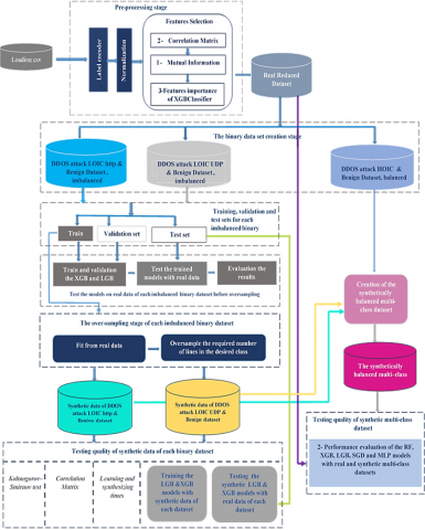
The approach we adopted in our research is depicted in Figure 4, and includes eight distinct stages. The pre-treatment constitutes the first stage which encompass label encoding, normalization and feature selection. The process of feature selection involves three techniques: correlation matrix, mutual information and feature importance based on the XGBoost classifier. The pre-processing stage ends with an evaluation of the relevance of the selected features. The second stage involves the creation of binary datasets. The third step involves the subdivision of each unbalanced binary dataset into separate training, validation, and testing subsets. Before applying oversampling, the fourth step is to test the models on real data from each unbalanced binary dataset. The fifth step is the data increase phase. The synthetic data quality tests for each binary data set are carried out in the sixth step. The seventh step involves the creation of the synthetically balanced multi-class dataset. Finally, the eighth step focuses on evaluating the effectiveness of the machine learning models across multi-class datasets, whether real or synthetic.
5.1 Pre-processing stage
After importing the csv files, we began the pre-processing stage, which includes data cleansing, label encoding, normalisation and feature selection. We began by cleaning up the data by first eliminating irrelevant columns. Next, we converted data with an inf value to a NAN value and then deleted all instances containing these values. For the encoding of class labels, we used the Label Encoder function from the sklearn.preprocessing library, which transforms categorical data into integer data. To improve the quality, performance, interpretability and explainability of the machine learning models, we opted to normalize the data using the StandardScaler function in the sklearn.preprocessing library. The aim of this approach is to eliminate problems relating to the scale of the variables, thereby facilitating a fair comparison between the different characteristics of the data. It aims to change the values of the numerical columns in the dataset using a common and uniform scale, preserving the range differences and avoiding information loss. Standard normalization, often referred to as standardization or z-score normalization, involves deducting the mean and then dividing by the standard deviation. In this way, each value represents the distance from the mean in units of standard deviation [38].
The standard normalization formula:
Transformed values $=\frac{\text { Values }- \text { Mean }}{\text { Standard Deviation }}$ (8)
5.1.1 Feature selection
For the feature selection process, we sequentially applied three specific techniques: the correlation matrix, Mutual Information and feature importance based on the XGBoost classifier.
The correlation matrix. one of the statistical techniques adapted in our study to the detection of DDoS attacks, is used to detect variables that are highly correlated with each other, which may indicate redundancies or interdependencies in the data and could introduce noise into the model. In our case study, we applied the correlation matrix to the dataset resulting from the preliminary pre-processing steps. This set comprises 80 normalized features. The matrix enabled us to identify the pairs of variables that are highly correlated, presenting correlation coefficients above the 0.95 threshold. Table 1 shows this result.
After applying the correlation matrix, only one of the two variables in each highly correlated pair is retained, while the other is removed from the data set. This process aims to eliminate information redundancy, as highly correlated features often provide similar information. So, by eliminating these highly correlated features, we have reduced dimensionality, retaining only information relevant to the machine learning model. This reduction can improve model performance and help prevent over-fitting. In addition, models are generally easier to interpret when features are independent or weakly correlated. Following the application of the correlation matrix, here are the 52 features retained in the dataset.
« 'Dst Port', 'Protocol', 'Flow Duration', 'Tot Fwd Pkts', 'Tot Bwd Pkts', 'Fwd Pkt Len Max', 'Fwd Pkt Len Min', 'Fwd Pkt Len Mean', 'Bwd Pkt Len Max', 'Bwd Pkt Len Min', 'Bwd Pkt Len Mean', 'Flow Byts/s', 'Flow Pkts/s', 'Flow IAT Mean', 'Flow IAT Std', 'Flow IAT Max', 'Fwd IAT Std', 'Bwd IAT Tot', 'Bwd IAT Mean', 'Bwd IAT Std', 'Bwd IAT Max', 'Bwd IAT Min', 'Fwd PSH Flags', 'Bwd PSH Flags', 'Fwd URG Flags', 'Bwd URG Flags', 'Bwd Pkts/s', 'Pkt Len Min', 'Pkt Len Var', 'FIN Flag Cnt', 'RST Flag Cnt', 'PSH Flag Cnt', 'ACK Flag Cnt', 'URG Flag Cnt', 'CWE Flag Count', 'Down/Up Ratio', 'Fwd Byts/b Avg', 'Fwd Pkts/b Avg', 'Fwd Blk Rate Avg', 'Bwd Byts/b Avg', 'Bwd Pkts/b Avg', 'Bwd Blk Rate Avg', 'Init Fwd Win Byts', 'Init Bwd Win Byts', 'Fwd Seg Size Min', 'Active Mean', 'Active Std', 'Active Max', 'Active Min', 'Idle Mean', 'Idle Std', 'Label'».
Figure 4. The approach followed for IDS optimization
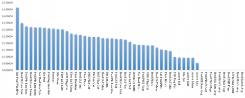
Figure 5. Visualization of features according to their importance measured by mutual information
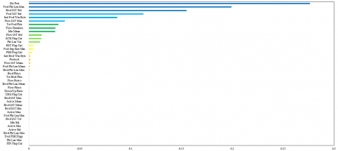
Figure 6. The importance of features, provided by the XGBoost model
Mutual information. In the second phase of our feature selection process, we used the mutual information technique on the dataset from the Correlation Matrix. This was done using the mutual_info_classif function in the sklearn.feature_selection library. Mutual information (MI) measures the dependency between two variables. We have used it to determine the impact of each feature on predicting the target variable, the class label. Regarding of DDoS attack detection, this technique is relevant because it identifies the variables that are most informative in predicting the class of DDoS attacks.
Mutual information measures the statistical dependence between two variables. In the context of machine learning, this measure assesses the dependency relationship between each feature and the class label variable, allowing us to measure how informative a particular feature is in predicting the class variable. The higher the mutual information, the more relevant the feature is considered to be for predicting the target variable. In this way, this measure helps to identify which features provide the most discriminating information on the presence or absence of a DDoS attack. Figure 5 facilitates the identification of the most informative features for the creation of predictive models in the context of our study.
In order to select the most informative features, we defined a selection threshold equal to 0.01. We retained 41 features whose mutual information with the label exceeded the defined threshold. The resulting dataset therefore includes the following 42 features: 'Dst Port', 'Protocol', 'Flow Duration', 'Tot Fwd Pkts', 'Tot Bwd Pkts', 'Fwd Pkt Len Max', 'Fwd Pkt Len Min', 'Fwd Pkt Len Mean', 'Bwd Pkt Len Max', 'Bwd Pkt Len Min', 'Bwd Pkt Len Mean', 'Flow Byts/s', 'Flow Pkts/s', 'Flow IAT Mean', 'Flow IAT Std', 'Flow IAT Max', 'Fwd IAT Std', 'Bwd IAT Tot', 'Bwd IAT Mean', 'Bwd IAT Std', 'Bwd IAT Max', 'Bwd IAT Min', 'Fwd PSH Flags', 'Bwd Pkts/s', 'Pkt Len Min', 'Pkt Len Var', 'RST Flag Cnt', 'ACK Flag Cnt', 'URG Flag Cnt', 'Down/Up Ratio', Init Fwd Win Byts', 'Init Bwd Win Byts', 'Fwd Seg Size Min', 'Active Mean', 'Active Std', 'Active Max', 'Active Min', 'Idle Mean', 'Idle Std', 'Label'.
Mutual information has proved invaluable in identifying influential features in class prediction. Its use reinforced the reduction of dimensionality and the retention of only the most informative features, contributing to the creation of a more succinct and refined dataset.
XGBoost feature importance. As part of the third feature selection method, we used the feature importance method of the XGBoost classifier. Feature importance is calculated by analyzing the contribution of each feature to the construction of the model's decision trees, thus providing indications as to which features are the most discriminating. The model assigns an importance score to each feature after training, measuring their contribution to the overall performance of the model. A major advantage of this classifier is its ability to prioritise features that increase predictive accuracy during training. In this phase, we trained the XGBoost model on the dataset resulting from the previous mutual information stage. By calculating and ranking the features according to their feature_importances, we were able to ascertain the significance of each feature for prediction. This is demonstrated in Figure 6, which identifies the most significant features for the XGBClassifier model, enabling us to establish a selection threshold at 0.001.
Applying this threshold, we selected 18 features with an importance greater than 0.001. We then checked that these selected features also had strong mutual information with the class label variable, indicating their predictive potential. This means that these features provide sufficient discriminant information to distinguish the different classes of the target variable.
Table 1. Pairs of highly correlated features following the correlation matrix
|
Feature1 |
Feature2 |
Correlation Value |
|
|
0 |
Flow Duration |
Fwd IAT Tot |
0.996960 |
|
1 |
Tot Fwd Pkts |
TotLen Fwd Pkts |
0.999216 |
|
2 |
Tot Fwd Pkts |
Fwd Header Len |
0.998923 |
|
3 |
Tot Fwd Pkts |
Subflow Fwd Pkts |
1.000000 |
|
4 |
Tot Fwd Pkts |
Subflow Fwd Byts |
0.999216 |
|
5 |
Tot Fwd Pkts |
Fwd Act Data Pkts |
0.999644 |
|
6 |
Tot Bwd Pkts |
TotLen Bwd Pkts |
0.996437 |
|
7 |
Tot Bwd Pkts |
Bwd Header Len |
0.999914 |
|
8 |
Tot Bwd Pkts |
Subflow Bwd Pkts |
1.000000 |
|
9 |
Tot Bwd Pkts |
Subflow Bwd Byts |
0.996437 |
|
10 |
TotLen Fwd Pkts |
Fwd Header Len |
0.997085 |
|
11 |
TotLen Fwd Pkts |
Subflow Fwd Pkts |
0.999216 |
|
12 |
TotLen Fwd Pkts |
Subflow Fwd Byts |
1.000000 |
|
13 |
TotLen Fwd Pkts |
Fwd Act Data Pkts |
0.999518 |
|
14 |
TotLen Bwd Pkts |
Bwd Header Len |
0.996341 |
|
15 |
TotLen Bwd Pkts |
Subflow Bwd Pkts |
0.996437 |
|
16 |
TotLen Bwd Pkts |
Subflow Bwd Byts |
1.000000 |
|
17 |
Fwd Pkt Len Max |
Fwd Pkt Len Std |
0.964655 |
|
18 |
Fwd Pkt Len Mean |
Fwd Seg Size Avg |
1.000000 |
|
19 |
Bwd Pkt Len Max |
Bwd Pkt Len Std |
0.969744 |
|
20 |
Bwd Pkt Len Max |
Pkt Len Max |
0.966422 |
|
21 |
Bwd Pkt Len Mean |
Pkt Len Mean |
0.951733 |
|
22 |
Bwd Pkt Len Mean |
Bwd Seg Size Avg |
1.000000 |
|
23 |
Bwd Pkt Len Std |
Pkt Len Max |
0.959944 |
|
24 |
Bwd Pkt Len Std |
Pkt Len Std |
0.953718 |
|
25 |
Flow Pkts/s |
Fwd Pkts/s |
0.989220 |
|
26 |
Flow IAT Mean |
Flow IAT Min |
0.988931 |
|
27 |
Flow IAT Mean |
Fwd IAT Mean |
0.989511 |
|
28 |
Flow IAT Mean |
Fwd IAT Min |
0.986116 |
|
29 |
Flow IAT Max |
Fwd IAT Max |
0.991463 |
|
30 |
Flow IAT Min |
Fwd IAT Mean |
0.965669 |
|
31 |
Flow IAT Min |
Fwd IAT Min |
0.988629 |
|
32 |
Fwd IAT Mean |
Fwd IAT Min |
0.977335 |
|
33 |
Fwd PSH Flags |
SYN Flag Cnt |
1.000000 |
|
34 |
Fwd Header Len |
Subflow Fwd Pkts |
0.998923 |
|
35 |
Fwd Header Len |
Subflow Fwd Byts |
0.997085 |
|
36 |
Fwd Header Len |
Fwd Act Data Pkts |
0.997376 |
|
37 |
Bwd Header Len |
Subflow Bwd Pkts |
0.999914 |
|
38 |
Bwd Header Len |
Subflow Bwd Byts |
0.996341 |
|
39 |
Pkt Len Max |
Pkt Len Std |
0.968040 |
|
40 |
Pkt Len Mean |
Pkt Size Avg |
0.992375 |
|
41 |
Pkt Len Mean |
Bwd Seg Size Avg |
0.951733 |
|
42 |
RST Flag Cnt |
ECE Flag Cnt |
0.999986 |
|
43 |
Subflow Fwd Pkts |
Subflow Fwd Byts |
0.999216 |
|
44 |
Subflow Fwd Pkts |
Fwd Act Data Pkts |
0.999644 |
|
45 |
Subflow Fwd Byts |
Fwd Act Data Pkts |
0.999518 |
|
46 |
Subflow Bwd Pkts |
Subflow Bwd Byts |
0.996437 |
|
47 |
Idle Mean |
Idle Max |
0.995137 |
|
48 |
Idle Mean |
Idle Min |
0.995723 |
|
49 |
Idle Max |
Idle Min |
0.982556 |
Table 2. The features in the reduced dataset after the three selection operations
|
NO. |
Position in CICIDS2018 |
Column |
Dtype |
|
1 |
1 |
Dst Port |
float64 |
|
2 |
2 |
Protocol |
float64 |
|
3 |
3 |
Flow Duration |
float64 |
|
4 |
5 |
Tot Fwd Pkts |
float64 |
|
5 |
9 |
Fwd Pkt Len Max |
float64 |
|
6 |
19 |
Flow IAT Mean |
float64 |
|
7 |
20 |
Flow IAT Std |
float64 |
|
8 |
21 |
Flow IAT Max |
float64 |
|
9 |
25 |
Fwd IAT Std |
float64 |
|
10 |
30 |
Bwd IAT Std |
float64 |
|
11 |
45 |
Pkt Len Var |
float64 |
|
12 |
48 |
RST Flag Cnt |
float64 |
|
13 |
49 |
PSH Flag Cnt |
float64 |
|
14 |
50 |
ACK Flag Cnt |
float64 |
|
15 |
68 |
Init Fwd Win Byt |
float64 |
|
16 |
69 |
Init Bwd Win Byt |
float64 |
|
17 |
71 |
Fwd Seg Size Min |
float64 |
|
18 |
76 |
Idle Mean |
float64 |
|
19 |
80 |
Label |
int64 |
Our approach was to sequentially combine these methods to obtain an optimal subset of relevant variables. First, we used the correlation matrix to remove highly correlated features, effectively reducing the data's dimensionality while retaining pertinent information. Next, we applied Mutual Information to assess the importance of the remaining features, selecting those that were most informative for predicting DDoS attacks. Finally, we used feature importance according to the XGBoost classifier to further refine the selection, focusing on the most discriminating features to improve model performance. Table 2 displays the breakdown of selected features following the implementation of the triple operation of selection. It includes the names of the features, their associated data type, as well as their position in the initial dataset of the CICIDS2018 DDOS attack.
We present below each of the characteristics of this reduced data set and how it could contribute to the detection of DDoS attacks:
Each selected characteristic from our reduced dataset offers a different perspective on network traffic, and can be used to detect anomalies or specific patterns of DDoS attacks. These features can all serve as potential indicators of an attack in progress. Combining these features in a machine learning model has the advantage of capturing complex malicious behavior and effectively detecting DDoS attacks. In this way, our feature selection methodology is based on solid principles and provides a robust framework for the proactive detection of DDoS attacks in computer networks.
Evaluation of selected features. We then investigated the reduced features to ensure that they retained sufficient information to ensure reliable detection of DDoS attacks. We also analyzed the impact of this reduction on the complexity of the model, the gain in execution time and the use of computational resources.
To verify the potential loss of information, we compared the performance of several machine learning models (RF, XGB, SGD, LGB and MLP) trained on the full dataset without feature reduction (0FS) with those trained on the reduced subset resulting from the three selection operations (3FS). Performance was evaluated using global metrics such as Accuracy, macro_accuracy, macro_recall and macro_F1-score. We also examined learning and prediction times in order to analyze the effect of the reduction on execution time.
5.2 Data balancing
The CICIDS2018 DDOS attack dataset shows a marked imbalance between classes, which can lead to a decrease in the performance of machine learning models, particularly for the minority class. ML models tend to be biased towards the majority class, which can lead to poor generalization for the minority class. With an unbalanced dataset, a model can achieve high accuracy (Accuracy) simply by consistently predicting the majority class. Furthermore, when the majority class is strongly represented, the model can overfit the data, leading to poor generalisation on the new data.
Balancing the class instances in a dataset enables a more accurate assessment of model performance and reduces the risk of overlearning. We opted for resampling techniques such as SMOTE, BorderlineSMOTE and ADASYN to resolve the class imbalance in our DDOS attack dataset. These methods generate synthetic examples based on the existing data of the minority class, preserving the underlying structure of the data while increasing the number of examples of that class. This approach helps to avoid the biases introduced by a radical modification of the data distribution. Compared with random oversampling, which can introduce duplicates and lead to overfitting, oversampling techniques such as SMOTE, BorderlineSMOTE and ADASYN generate synthetic examples in a more targeted way, improving the ability of models to generalize to real data. Indeed, these resampling techniques create synthetic examples, using methods that preserve the meaning of existing data. By way of illustration, SMOTE generates new examples by performing a linear interpolation between several existing examples of the minority class, located in a defined neighborhood. This ensures that the synthetic data remains consistent with the real characteristics of the data. Furthermore, by generating synthetic examples for minority classes, these oversampling techniques improve the diversity of the training data, essential for generalizing to new examples. They also balance the distribution of classes without introducing excessive biases, thus reducing the risk of over-fitting models to majority classes. What's more, these techniques offer control over the generation of synthetic data, allowing parameters such as the level of oversampling or the neighbor selection method to be adjusted in order to optimize results. In sum, resampling techniques offer a flexible and effective approach to managing class imbalance, preserving data distribution and improving the ability of models to detect examples of minority classes.
In our research, we used resampling techniques to balance our reduced dataset. We divided the dataset into three binary datasets, each consisting of a "Benign" class and an attack class. Using the "sample" function, we randomly subsampled instances of the majority "Benign" class to obtain 686012 instances in each binary set. This process was repeated three times to create three binary sets. We associated each attack class in the reduced dataset with a subsample of the "Benign" class to form binary datasets. The three binary datasets resulting from this division are as follows:
The first unbalanced dataset, named dfbehttp, consists of: 686012 benign instances and 576191 DDoS-LOIC-HTTP attack samples, it has an imbalance ratio = 1.190. The second unbalanced dataset, called dfbeudp, consists of 686012 benign instances and 1730 DDOS-LOIC-UDP attacks, it has an imbalance ratio=396.538. The third data set, named dfbehoic, is balanced and consists of 686012 benign observations and 686012 DDOS-HOIC attack samples.
First, we divided each unbalanced binary dataset into a training set and a test set, the latter representing 12% of instances. Then, from each training set, a validation set representing 18% of the data was extracted we extracted a validation set comprising 18% of the data. To assess the quality of the synthetic data to be generated, we first trained, validated and tested the XGB and LGB classifiers on the real data from these sets.
To tackle the class imbalance in the binary datasets dfbehttp and dfbeudp, we generated 109,821 instances for the LOIC-HTTP class in the dfbehttp dataset and 684,282 instances for the LOIC-UDP class in the dfbeudp dataset to achieve to balance these two datasets. We used the oversampling techniques of the Python "imbalanced-learn" library, including the Synthetic Minority Oversampling Technique (SMOTE) and its variants ADASYN (Adaptive Synthetic Sampling Approach) and BorderlineSMOTE. We were able to apply the SMOTE method to both datasets. However, the variants could not only be tested on the dfbehttp dataset because running each of them on the dfbeudp dataset generated an error message for ADASYN indicating that the variant was not suitable for this specific dataset and that SMOTE should be used instead. As for BorderlineSMOTE, it did not result in oversampling for the LOIC-UDP class of DDOS attack, leaving the number of observations for this class unchanged. As a result, we only used the SMOTE technique to generate instances for the dfbeudp dataset.
The underlying theory behind the SMOTE, ADASYN and BorderlineSMOTE oversampling techniques may help explain why SMOTE was able to generate synthetic data for the LOIC HTTP and LOIC UDP classes, while ADASYN and BorderlineSMOTE only generated synthetic data for the LOIC HTTP class. SMOTE works by generating synthetic examples by linearly interpolating between examples of the minority class in feature space. This technique is generally effective when the examples of the minority class are close to each other in feature space. In the case of the LOIC HTTP and LOIC UDP classes, SMOTE was able to generate synthetic data because the examples of these classes were probably close enough to each other to allow linear interpolation. ADASYN adapts the oversampling rate for each example in the minority class according to the local density of examples in that class. This means that ADASYN tries to generate more synthetic examples where there are fewer real examples of the minority class. In the case of the LOIC UDP class, where there are very few real examples, ADASYN may struggle to generate efficient synthetic data as it is difficult to estimate the local density in these sparsely populated regions of the feature space. BorderlineSMOTE generates synthetic examples only from those examples of the minority class that are close to the decision boundary between classes. In the case of the LOIC UDP class, where the imbalance is very marked, it's possible that the examples of this class are very far from the decision frontier, which would explain why BorderlineSMOTE didn't generate synthetic examples for this class.
Table 3. The techniques used for oversampling the minority classes of the dfbehttp and dfbeudp datasets
|
Test Number |
LOIC-Http Class of DDoS Attacks for the Dfbehttp |
LOIC-UDP Class of DDOS Attacks for the Dfbeudp |
|
config 1 |
SMOTE |
SMOTE |
|
config 2 |
ADASYN |
SMOTE |
|
config 3 |
BorderlineSMOTE |
SMOTE |
The different configurations tested are summarized in Table 3.
To assess the quality of the synthetic data generated, we carried out several tests on the data generated by each of the above-mentioned configurations and relating to the two imbalanced binary datasets dfbehttp and dfbeudp.
Firstly, we used the Kolmogorov-Smirnov (KS) test, which assesses the similarity between two cumulative probability distributions [39], It assesses the normality of a distribution by comparing an empirical distribution with a reference distribution (usually a theoretical distribution), in order to detect any significant deviation in the data. In our research, this method is used to assess the similarity between the distributions of real data and synthetically generated data. This evaluation is necessary because it is important to ensure that the synthetic data preserves the fundamental characteristics of the real data, this is essential for the reliability of our DDoS attack detection models. This test is also used to determine whether two independent samples come from the same population, or whether they show significant differences, which is particularly useful in comparative studies [40]. Next, we explored the correlation matrix to analyze the linear relationships between the variables. Comparing the correlation matrices of the real and synthetic data allowed us to determine whether the relationships between the variables were correctly reproduced by the synthetic data. As a third test, we evaluated the performance of the XGB and LGB models using first the real data for training and then the synthetic data. This allowed us to compare the performance of the synthetic models with that of the real models and to assess the generalizability of the synthetic models on real-world data. To evaluate these performances, we used the AUC_ROC and macro f1_score metrics. Lastly, we considered the training and synthesis times to assess the operational efficiency of synthetic generation methods.
Next, we combined the syn_dfbeudp and syn_dfbehttp synthetic datasets with the remaining dfbehoic dataset, forming a balanced, synthetic and global dataset that includes both real and synthetic data. The Figure 7 shows the synthetically balanced dataset.
Then, to evaluate this global synthetic dataset, we compared how well the models (MLP, LGB, RF, XGB, and SGD) performed. Firstly, the machine learning models were initially trained on the real data. Then, they were re-trained on the synthetic data and, finally, evaluated in both cases using the real test data. This evaluation focused on studying the behaviour of the models, analysing both the overall performance and the performance per class on the real test data before and after synthesising the data.
To carry out this evaluation, we first divided the reduced global dataset of real data into training and test sets, the second set representing 12% of the data. Next, we trained the aforementioned machine learning models on the training set of real data using the Stratified K-Folds cross-validator technique with n_splits=5. This method divides the dataset into folds to evaluate the performance of a model that ensures a balanced distribution of classes in each fold, thus guaranteeing a robust evaluation even when the classes are not uniformly distributed. After training, the models were tested with real test data. Next, the same models were re-trained on the global synthetic dataset, also using StratifiedKFold with n_splits=5. Finally, the performance of these synthetic models was evaluated with test data and real data to check their performance with real data and verify whether the synthetic data succeeded in capturing the features important for DDOS attack detection. The evaluation metrics used in this step are precision, sensitivity, F1_score and false positive rate (FPR). Execution times for learning and prediction were also taken into account.
The approach used in our study is based on a holistic strategy aimed at improving the robustness and effectiveness of anomaly-based intrusion detection systems in detecting DDOS attacks. To achieve this goal, we have combined several key techniques, including feature selection, data resampling (undersampling and oversampling) and the use of advanced classification algorithms.
Figure 7. The synthetically balanced CICIDS 2018 DDOS attack dataset
Firstly, feature selection was carried out by sequentially applying three specific techniques: correlation matrix, Mutual Information and feature importance according to the XGBoost classifier. This triple feature selection operation created an optimal subset of relevant variables, contributing to a more concise representation of the data. Then, to cope with the class imbalance in our dataset, we used oversampling techniques such as SMOTE, ADASYN and BorderlineSMOTE. These methods were applied in a targeted manner to each binary dataset, focusing on the specific characteristics of each attack class. This enabled us to generate synthetic data that faithfully captured the characteristics of each attack type, thereby increasing the diversity of the training data and improving the ability of the models to generalize to new examples. Finally, we used advanced classification algorithms such as RF, XGB, SGD, LGB and MLP to train our models. These algorithms were evaluated on the global synthetic and balanced dataset resulting from merging the binary sets after oversampling. The performance of each algorithm was analyzed based on detection rate (precision, recall and f1_score), false positive rate and execution time. By combining these different techniques, our methodology aims to make the most of the complementary nature of the feature selection, oversampling and classification approaches, in order to optimize model performance in the detection of DDoS attacks.
6.1 Setting up hardware and the operating environment
The empirical study conducted in this research work used the Google Colab Pro+ platform to perform the experiments and answer the questions we were posed. it's an online machine learning environment offering hosted Jupyter notebooks with no configuration required and high RAM capacity, including access to GPUs and TPUs. The models were developed, trained, evaluated and tested using the Scikit-Learn library, which is an open source Python library for machine learning based on NumPy, SciPy and Matplotlib. These libraries provide essential functionality for data processing, scientific calculations and visualisation, enabling Scikit-Learn to implement many machine learning algorithms and associated tools. We have used various Scikit-Learn modules for pre-processing, feature selection, model selection, as well as for the implementation of different classification methods (RF, SGD, MLP) and performance evaluation. In addition, we have integrated the open source Imbalanced-learn library (under the name imblearn) to handle unbalanced datasets using oversampling techniques such as SMOTE, BorderlineSMOTE and ADASYN. We used the LightGBM and XGBoost machine learning algorithm modules, the latter also for feature selection. For KS testing, we used the scipy.stats library. Finally, to analyse and visualise the data, we used the Python libraries NumPy, Pandas and Matplotlib.
6.2 Performance metrics
In order to evaluate the performance of the machine learning models used to test synthesizing, we used the following metrics: accuracy, precision, recall, F1-score, macro-accuracy, macro-recall, macro F1-score and area under the ROC curve (ROC AUC). These measures are based on different combinations of confusion matrix elements (TP, TN, FP, FN). TP indicates the number of correct predictions of the positive class, TN indicates the number of correct predictions of the negative class, FP refers to the count of erroneous classifications where a negative instance is identified as positive, while FN represents the number of incorrect predictions where a positive sample is mistakenly classified as negative.
Accuracy is the ratio between the number of correctly predicted normal and abnormal data (TN and TP) and the total number of predictions made. It assesses the overall accuracy of a classification model.
Accuracy $=\frac{T P+T N}{F P+F N+T P+T N}$ (9)
Precision represents the ratio of true positives to the total number of positives predicted. It assesses the reliability of positive predictions, focusing on Type I (FP) errors.
Precision $=\frac{T P}{T P+F P}$ (10)
Macro-precision is the average precision for each class in a multi-class classification problem, providing an overall assessment of prediction reliability for all classes.
Recall, also called true positive rate (TPR) or sensitivity, evaluates the model's ability to correctly detect all positive instances among all truly positive instances.
Recall $=\frac{T P}{T P+F N}$ (11)
Macro-recall is the average recall for each class in a multi-class classification problem, offering an overall assessment of the model's ability to correctly identify all positive instances of each class.
The F1 score is the harmonic mean of precision and recall. This measure provides a balance between precision and recall, offering an overall assessment of classification performance.
$f 1-$ score $=\frac{2 *(\text { Precision } * \text { Recall })}{(\text { Precision }+ \text { Recall })}$ (12)
The Macro F1-score represents the harmonic mean between macro-precision and macro-recall, giving a single measure balancing precision and recall for each class, valuable for evaluating the overall performance of multi-class classification.
The false positive rate (FPR) is calculated as the number of false positives divided by the total number of negative instances in a dataset. It assesses a model's effectiveness in correctly identifying negative instances.
$F P R=\frac{F P}{F P+T N}$ (13)
The area under the ROC curve (ROC AUC) measures a model's ability to correctly classify positive versus negative instances, giving an overall measure of binary classification model performance.
6.3 Experimentation, outcomes and discussion
During the experiment to evaluate the reduced features, we observed a significant difference in resource requirements when normalizing the data. The initial dataset required 70GB of RAM, while the reduced dataset consumed only 29.6GB of RAM. We then divided each dataset (initial and reduced) into a training set (70%) and a test set (30%). When evaluating the overall performance of the models (RF, XGB, SGD, LGB and MLP) on the test datasets, we found that most of the models using the reduced dataset performed similarly compared to those using the original dataset, or even better, as seen with the MLP classifier. Figure 8 shows the performance results of the models before and after feature selection for the chosen metrics.
Figure 8. The performance of the RF, XGB, SGD, LGB and MLP models before and after feature selection
Figure 9. Variations in ML model runtimes between Initial and Reduced datasets
As for the evaluation of execution times, we observed that the total duration, including learning and prediction times, halved for all models, with the exception of the MLP model, where it increased. This evaluation of the execution time of the models before and after feature selection is presented in Figure 9.
The inherent complexity of the MLP model, with its hidden layers and numerous parameters to adjust, can explain the extended execution time when using reduced data. This complexity requires more time to adapt the MLP to the reduced data while maintaining high performance. However, the observed increase in performance suggests that feature selection has been beneficial.
In order to assess the quality of the synthetic data obtained by applying the data increase techniques (SMOTE, BorderlineSMOTE or ADASYN) to the real data from the LOIC-HTTP and LOIC-UDP classes of DDOS attack, we carried out several tests on both the binary synthetic datasets and the multi-class synthetic dataset.
6.3.1 Evaluations on binary datasets
Kolmogorov Smirnov test. In our evaluations on synthetically balanced binary datasets, we used the Kolmogorov-Smirnov test to compare the distributions of the synthetic data with the distributions of the real data. The results are shown in Table 4 and Table 5
Regarding the LOIC-HTTP class of DDoS attacks, we observed that the SMOTE method has the lowest KS_statistics values compared to the other two methods, ADASYN and BorderLine, indicating that the synthetic data generated by SMOTE is closest to the real data for this class. In contrast, we found that the distributions of synthetic features for the LOIC-UDP class of DDoS attack are further away from the distribution of real data compared to the LOIC-HTTP class of DDoS attacks. This finding suggests a divergence in the feature distribution of this class compared to the real data.
Comparison of correlation matrices. The second test we conducted involves of comparing the correlation matrices. This analysis is essential because it enables us to assess the preservation of the relationships between the variables when synthesizing the data.
Figure 10 illustrates the correlation matrices of both the real and synthetic data for the LOIC-HTTP class of DDoS attack following the execution of the SMOTE, BorderlineSMOTE and ADASYN oversampling techniques. Visually, the correlation matrices of the synthetic data are similar to those of the real data, indicating that all three synthesis methods preserved all the linear relationships between the variables present in the real data of the DDoS attack LOIC-HTTP class.
Figure 11 shows the correlation matrices of the real and synthetic data for the LOIC-UDP class of DDoS attacks. We note that in the synthetic correlation matrix for this class of DDoS attack, the majority of linear relationships between features in the real correlation matrix are preserved. However, we also note the emergence of new relationships. This observation can be explained by the substantial increase of 684282 instances for this class.
Evaluation of model performance on synthetic binary datasets. For each synthesizing method, we evaluated the performance of the XGB and LGB models, before and after generation, for the datasets relating to each of the DDOS attack classes LOIC-http and LOIC-UDP. This evaluation was carried out using a real test dataset specific to each class, applied to the associated real and synthetic models. The assessment metrics used include Accuracy, ROC_auc and macro_f1_score. The outcomes for synthesizing the dfhttp dataset are presented in Table 6, while those for synthesizing the dfbeudp dataset appear in Table 7.
Table 4. Results of the KS test for the LOIC-HTTP class of DDOS attack
|
KS-Statistic DDOS attack LOIC-HTTP |
|||
|
Column |
SMOTE |
BorderlineSMOTE |
ADASYN |
|
Dst Port |
0.023801 |
0.023801 |
0.023794 |
|
Protocol |
0.014198 |
0.014295 |
0.012985 |
|
Flow Duration |
0.027785 |
0.046384 |
0.035082 |
|
Tot Fwd Pkts |
0.016297 |
0.032933 |
0.032832 |
|
Fwd Pkt Len Max |
0.034014 |
0.052691 |
0.051370 |
|
Flow IAT Mean |
0.029248 |
0.034208 |
0.021132 |
|
Flow IAT Std |
0.012769 |
0.036087 |
0.035985 |
|
Flow IAT Max |
0.029782 |
0.045402 |
0.035474 |
|
Fwd IAT Std |
0.016803 |
0.032920 |
0.032819 |
|
Bwd IAT Std |
0.014723 |
0.033361 |
0.033351 |
|
Pkt Len Var |
0.017811 |
0.052338 |
0.052323 |
|
RST Flag Cnt |
0.012019 |
0.028345 |
0.028337 |
|
PSH Flag Cnt |
0.003937 |
0.036428 |
0.036418 |
|
ACK Flag Cnt |
0.011229 |
0.051690 |
0.050370 |
|
Init Fwd Win Byts |
0.022441 |
0.054127 |
0.055325 |
|
Init Bwd Win Byts |
0.014228 |
0.039986 |
0.039974 |
|
Fwd Seg Size Min |
0.015016 |
0.015113 |
0.013803 |
|
Idle Mean |
0.013301 |
0.015461 |
0.016670 |
Table 5. Results of the KS test for the LOIC-UDP class of DDOS attack
|
KS-Statistic DDOS attack LOIC-UDP |
|
|
Column |
SMOTE |
|
Dst Port |
0.271756 |
|
Protocol |
0.334688 |
|
Flow Duration |
0.460121 |
|
Tot Fwd Pkts |
0.497359 |
|
Fwd Pkt Len Max |
0.352893 |
|
Flow IAT Mean |
0.274427 |
|
Flow IAT Std |
0.285545 |
|
Flow IAT Max |
0.333415 |
|
Fwd IAT Std |
0.317059 |
|
Bwd IAT Std |
0.171214 |
|
Pkt Len Var |
0.387959 |
|
RST Flag Cnt |
0.113825 |
|
PSH Flag Cnt |
0.206268 |
|
ACK Flag Cnt |
0.117379 |
|
Init Fwd Win Byts |
0.325373 |
|
Init Bwd Win Byts |
0.246794 |
|
Fwd Seg Size Min |
0.325373 |
|
Idle Mean |
0.073201 |
(a) Real data
(b) Synthetic data generated by SMOTE
(c) Synthetic data generated by BorderlineSMOTE
(d) Synthetic data generated by Adasyn
Figure 10. The correlation matrices of the real and synthetic data for the LOIC-HTTP class of DDoS attack following execution of oversampling techniques
(a) Real data
(b) Synthetic data generated by SMOTE
Figure 11. Correlation matrices of the real and synthetic binary datasets corresponding to the LOIC-UDP DDoS attack class
Table 6. Outcomes of synthesizing the dfbehttp dataset for the LGB and XGB models
|
Synthetization Method |
Model |
Accuracy |
Roc_auc |
Macro f1_Score |
|
SMOTE |
LGB_http_BS |
99.97% |
99.97% |
99.97% |
|
LGB_http_AS |
99.96% |
99.97% |
99.96% |
|
|
XGB_http_BS |
100% |
100% |
100% |
|
|
XGB_http_AS |
100.00% |
100% |
100% |
|
|
Borderline SMOTE |
LGB_http_BS |
99.97% |
99.98% |
99.97% |
|
LGB_http_AS |
99.98% |
99.98% |
99.98% |
|
|
XGB_http_BS |
100% |
100% |
100% |
|
|
XGB_http_AS |
100% |
100% |
100% |
|
|
ADASYN |
LGB_http_BS |
99.96% |
99.97% |
99.96% |
|
LGB_http_AS |
99.98% |
99.98% |
99.98% |
|
|
XGB_http_BS |
100% |
100% |
100% |
|
|
XGB_http_AS |
100% |
100% |
100% |
BS: Before synthesis-AS: After synthesis
Table 7. Results of synthesizing the dfbeudp dataset for the LGB and XGB models
|
Synthetization Method |
Model |
Accuracy |
Roc_auc |
Macro f1_Score |
|
SMOTE |
LGB_udp_BS |
100% |
99.53% |
99.88% |
|
LGB_udp_AS |
100% |
100% |
100% |
|
|
XGB_udp_BS |
100% |
100% |
100% |
|
|
XGB_udp_AS |
100% |
100% |
100% |
Table 8. The results for learning times and synthetic data generation for the dfbehttp and dfbeudp datasets
|
Dataset |
Synthetization Method |
Learning and Synthetic Data Generation Times in Seconds |
|
dfbehttp |
SMOTE |
271.475 |
|
BorderlineSMOTE |
644.242 |
|
|
ADASYN |
1042.087 |
|
|
dfbeudp |
SMOTE |
0.513 |
|
SMOTE |
0.527 |
|
|
SMOTE |
0.755 |
Table 9. Global performance results of models before and after synthesizing
|
Model and Ssynthesizing Combinations |
Accuracy |
Macro Precision |
Macro Recall |
Macro f1_Score |
|
RF_Real_data |
1 |
0.96 |
0.98 |
0.97 |
|
RF_SMOTE SMOTE |
1 |
0.97 |
1 |
0.98 |
|
RF_BorderlineSmote SMOTE |
1 |
0.97 |
1 |
0.98 |
|
RF_Adasyn SMOTE |
1 |
0.97 |
1 |
0.98 |
|
XGB_Real _data |
1 |
0.96 |
0,98 |
0.97 |
|
XGB_SMOTE SMOTE |
1 |
0.95 |
1 |
0.97 |
|
XGB_BorderlineSmote SMOTE |
1 |
0.95 |
1 |
0.97 |
|
XGB_Adasyn SMOTE |
1 |
0.95 |
1 |
0.97 |
|
SGD_Real _data |
0.99 |
0.89 |
0.88 |
0.88 |
|
SGD_SMOTE SMOTE |
0.95 |
0.82 |
0.99 |
0.89 |
|
SGD_BorderlineSmote SMOTE |
0.95 |
0.82 |
0.99 |
0.88 |
|
SGD_Adasyn SMOTE |
0.95 |
0.82 |
0.99 |
0.88 |
|
LGB_Real _data |
1 |
0.74 |
0.74 |
0.74 |
|
LGB_SMOTE SMOTE |
0.9 |
0.64 |
0.97 |
0.71 |
|
LGB_BorderlineSmote SMOTE |
0.99 |
0.76 |
1 |
0.76 |
|
LGB_Adasyn SMOTE |
1 |
0.87 |
1 |
0.91 |
|
MLP_Real _data |
1 |
0.94 |
0.99 |
0.96 |
|
MLP_SMOTE SMOTE |
1 |
0.93 |
1 |
0.96 |
|
MLP_BorderlineSmote SMOTE |
0.96 |
0.84 |
0.99 |
0.9 |
|
MLP_Adasyn SMOTE |
1 |
0.93 |
1 |
0.96 |
The results show a similarity in the performance of the LGB and XGB models before and after synthesizing, whether for the three methods applied to dfbehttp or for the SMOTE method applied to dfbeudp, with a slight improvement for LGB. This similarity suggests that the synthetically generated data effectively retains the characteristics of the real data.
Evaluation of learning and synthesis times. In our evaluation, we have taken into account the time required to learn from real data and to generate synthetic data. The aim of this evaluation is to measure the operational efficiency of synthetic data generation methods by analyzing the time required to train models on real data and to produce synthetic data. This analysis makes it possible to understand the differences in performance between the methods, which is important for choosing the optimum approach according to the time constraints specific to each project. Significant differences in learning times between methods can impact on the practicality and overall efficiency of models, underlining the importance of these aspects when choosing the synthetic generation method.
Table 8 shows the results for learning times and synthetic data generation for the two datasets, dfbehttp and dfbeudp, using different synthesis methods.
For dfbehttp, we observe that ADASYN requires significantly more learning time (1042.087seconds) compared to SMOTE (271.475seconds) and BorderlineSMOTE (644.242seconds). However, all the methods produce balanced synthetic data after sampling, maintaining an equal number of instances for each class. For dfbeudp, the learning times with SMOTE vary slightly (0.513, 0.527, and 0.755 seconds). A significant difference is also noted in the training and synthetic data generation times between the two datasets dfbehttp and dfbeudp, which could be attributed in part to the imbalance in the number of initial instances for class "1". The fact that dfbehttp has a minority class with 506979 instances, while dfbeudp has only 1517, may influence the time taken for the synthesis methods to balance the classes. A high initial number of instances can potentially require more time to generate synthetic data while maintaining balance.
Figure 12. Synthesizing results on the benign class
Figure 13. Results of synthesizing on the HOIC class of DDOS attack
6.3.2 Model evaluation on synthetically balanced multi-class datasets
To form the synthetically balanced multi-class datasets of CICIDS2018 DDOS attacks, we used the oversampling techniques SMOTE, Borderline SMOTE and ADASYN. Each multi-class dataset was created by merging the synthetically balanced binary datasets (dfbehttp_syn and dfbeudp_syn) with the real, balanced dataset (dfbehoic). These synthetic multi-class datasets comprise the classes generated by different combinations of synthesis methods, namely (SMOTE; SMOTE), (ADASYN; SMOTE) and (BorderlineSMOTE; SMOTE), applied respectively to the DDOS attack classes, namely the LOIC-http class of the dfbehttp dataset and the LOIC-UDP class of the dfbeudp dataset. Each multi-class synthetic dataset corresponds to one of the aforementioned combinations.
To select the most optimal combination of synthesis methods that we used to increase the representation of minority classes and improve the balance between classes, we evaluated the performance of the RF, XGB, SGD, LGB and MLP models. This evaluation was carried out both on the reduced global real dataset and on the synthetic multi-class datasets produced by the different synthesizing combinations such as (SMOTE_SMOTE), (ADASYN_SMOTE) and (BorderlineSMOTE_SMOTE). Performance was evaluated using real test data, a crucial approach for ensuring that models trained on synthetic data generalize effectively in real-life situations. This method avoids any biases or artificial relationships introduced by synthetic data. Testing on real data allows the robustness and effectiveness of the model to be validated under a wider range of conditions, ensuring a more reliable assessment of its performance and applicability under a variety of practical conditions.
Regarding the evaluation of overall model effectiveness, Table 9 presents the global outcomes of the RF, XGB, SGD, LGB and MLP models on real test data before and after data synthesis. The evaluation was conducted using the global indicators Accuracy, macro_precision, macro_recall and macro_f1 score. These indicators provide an overall view of the behavior of these models.
For the RF and XGB classifiers, the effectiveness of the synthesized data is similar to that of the real data. However, for the SGD model, the performance of the synthetic data is generally inferior or equal to that of the real data, with the exception of recall. As for the LGB model, the "ADASYN, SMOTE" combination shows synthetic data performance superior to real data, while performance for the "BorderlineSMOTE, SMOTE" combination is equivalent, and for the "SMOTE, SMOTE" combination it is inferior to real data, with the exception of recall. As for the MLP model, the performance of the synthetic data for the "BorderlineSMOTE, SMOTE" combination is inferior to that of the real data, while for the other two synthesizing combinations, it is equivalent.
In general, the metrics appear stable or show slight variation after synthesizing, suggesting that overall model performance is not significantly affected by the introduction of synthetic data. This indicates that the synthetically generated data succeeded in maintaining the generalization capability of the models, producing results consistent with those obtained on real data.
Evaluation of model performance by class. Looking more closely at the performance evaluation of the models by class, we observed different trends according to the combinations of synthesis methods. For the "Benign" class, whose results are presented in Figure 12, the SGD and LGB models showed inferior performance for the "SMOTE_SMOTE" combination, while the other models achieved similar performance between real and synthetic data. With the "BorderlineSMOTE, SMOTE" combination, RF, XGB and LGB showed stable performance, but SGD and MLP showed weaker performance for synthetic data. For the "ADASYN, SMOTE" combination, performance was comparable between real and synthetic data for RF, XGB, LGB and MLP, but slightly lower for SGD.
In summary, synthetic data performance is stable for RF and XGB, variable for LGB and MLP depending on the combination, while SGD consistently shows lower performance with all combinations. The "ADASYN, SMOTE" combination stands out as presenting the most models with stable performance between real and synthetic data, suggesting good prediction quality while balancing the data.
Models performances results for the HOIC class of DDOS attacks after the data synthesis corresponding to combinations of SMOTE, BorderlineSMOTE and ADASYN techniques, are presented in Figure 13.
The "ADASYN, SMOTE" and "BorderlineSMOTE, SMOTE" combinations showed identical performance between synthetic and real data, with even an improvement for the synthetic LGB model. The "SMOTE, SMOTE" combination also performed similarly, but with a decrease in performance for the synthetic LGB model. For the SGD classifier, all combinations resulted in a reduction in precision after synthesizing.
The LOIC-UDP minority class of DDoS attacks benefited from an increase in data thanks to data synthesis. The performance of models with the SMOTE, BorderlineSMOTE and ADASYN synthesis combinations on this class is displayed in Figure 14.
Figure 14. Synthesized results on the LOIC-UDP class of DDOS attack
For RF, the performance of the synthetic data is better for all three combinations. The XGB model shows superior recall and F1-score results with synthetic data for all three combinations. SGD performance increases for all metrics and combinations. The LGB model shows zero performance with real data, but synthesizing improves this performance.
The "ADASYN, SMOTE" combination proved to be the most efficient, followed by "SMOTE, SMOTE". For the MLP model, performance is identical between real and synthetic data for all combinations. Overall, the increase in data led to an improvement in performance for this minority class, and the "ADASYN, SMOTE" combination stood out as the most efficient compared with the other two combinations.
The DDOS attack LOIC-HTTP class also benefited from an increase in data. Figure 15 displays the performance results of the models before and after the synthesis on the LOIC-HTTP class. The efficiency of the synthetic data for the RF and XGB models is found to be identical to that of the real data for the three synthesizing combinations.
Figure 15. Synthesized results on the LOIC-HTTP class of DDOS attack
Concerning the SGD model, all three variants showed a decrease in precision and F1 score, but an improvement in recall. LGB slightly improved its performance with the "ADASYN, SMOTE" and "BorderlineSMOTE, SMOTE" combinations, while "SMOTE, SMOTE" led to a deterioration. MLP achieved similar performance between real and synthetic data for "SMOTE, SMOTE" and "ADASYN, SMOTE", but a decrease in precision and f1_score for "BorderlineSMOTE, SMOTE".
In summary, the "ADASYN, SMOTE" combination presented the most synthetic models with performance equivalent to real data for the DDOS attack LOIC-HTTP class, with an additional performance improvement for the LGB model.
Evaluation of false positive rates. Still with a view to evaluating the performance of the models, we also tested the false positive rates obtained by the five models before and after synthesizing. Table 10 below provides information on the results of these tests.
The results show an overall trend towards a decrease in the false positive rate (FPR) for the "Benign" class after applying different synthesizing methods, suggesting an improvement in the models' ability to correctly classify the majority class. The LGB model showed significant decreases in FPR, especially for the "ADASYN; SMOTE" and "BorderlineSMOTE; SMOTE" synthesizing combinations, highlighting the effectiveness of these methods in enhancing the accuracy of the LGB model in classifying the Benign class and DDoS attack classes HOIC and LOIC-HTTP. However, the "SMOTE; SMOTE" combination led to a substantial rise in the FPR for the LGB model, indicating a particular sensitivity to this synthesizing method. On the other hand, the SGD model stood out, showing an increase in FPR for all synthesizing combinations, which is consistent with previous results indicating a decrease in performance for this model in the synthetic context. These observations underline the importance of choosing the right synthesizing method for specific models. Finally, synthesizing the data using the "SMOTE; SMOTE", "ADASYN; SMOTE" and "BorderlineSMOTE; SMOTE" combinations improved model performance by reducing false positives for the "Benign" negative class.
Evaluation of runtimes. As part of our evaluation of the overall performance of the RF, XGB, SGD, LGB and MLP models on real test data before and after synthesizing the data, we also tested the runtimes of the real and synthetic models (taking into account the training, validation and test runtimes) for each synthesizing combination. Figure 16 shows the results of these runtime tests. Firstly, we note that the MLP model followed by the RF model take the longest time to execute, and that the synthetic models have a significantly shorter execution time than the real models.
Faster convergence of synthetic models during training can lead to faster optimized performance, as synthetic data, often balanced and homogeneous, reduces noise and outliers, enabling the model to identify relevant relationships in the data and fit more efficiently. This homogeneity stabilizes gradients, speeding up the optimization process and reducing the number of iterations needed to achieve optimal performance. As a result, models converge faster, require fewer computing resources and deliver better performance in less time.
This significant reduction in execution times can be interpreted as a major practical advantage, suggesting that models based on synthetic data can be more efficient in regard of time resources, which can be particularly decisive in operational contexts where time is a constraint.
Table 10. Results of the false-positive rates obtained by the models before and after synthesizing
|
FPR Results-Before Synthesizing |
FPR Results-After Synthesizing |
||||||||
|
Synthetization Combinaison |
Model |
Benign |
DDOS Attack-HOIC |
DDOS Attack-LOIC-UDP |
DDoS Attacks-LOIC-HTTP |
Benign |
DDOS Attack-HOIC |
DDOS Attack-LOIC-UDP |
DDoS Attacks-LOIC-HTTP |
|
SMOTE, SMOTE |
RF |
2,62E-05 |
0,00E+00 |
4,01E-05 |
1,69E-05 |
0,00E+00 |
0,00E+00 |
2,80E-05 |
2,39E-05 |
|
XGB |
1,31E-05 |
0,00E+00 |
3,92E-05 |
1,79E-05 |
0,00E+00 |
3,03E-06 |
4,66E-05 |
0,00E+00 |
|
|
SGD |
5,18E-02 |
4,72E-03 |
6,34E-05 |
1,82E-03 |
7,87E-05 |
5,10E-03 |
7,65E-05 |
4,30E-02 |
|
|
LGB |
1,20E-02 |
4,12E-04 |
9,14E-05 |
2,23E-03 |
3,48E-04 |
4,51E-03 |
7,08E-04 |
1,00E-01 |
|
|
MLP |
2,44E-03 |
4,04E-06 |
6,43E-05 |
1,37E-04 |
8,66E-04 |
4,04E-06 |
7,37E-05 |
9,00E-04 |
|
|
BorderlineSMOTE, SMOTE |
RF |
1,97E-05 |
0,00E+00 |
4,01E-05 |
1,99E-05 |
0,00E+00 |
0,00E+00 |
3,26E-05 |
1,59E-05 |
|
XGB |
1,31E-05 |
0,00E+00 |
3,92E-05 |
1,79E-05 |
0,00E+00 |
3,03E-06 |
4,48E-05 |
9,97E-07 |
|
|
SGD |
5,17E-02 |
4,71E-03 |
6,34E-05 |
1,85E-03 |
7,87E-05 |
5,03E-03 |
7,65E-05 |
4,45E-02 |
|
|
LGB |
1,20E-02 |
4,12E-04 |
9,14E-05 |
2,23E-03 |
2,56E-04 |
1,11E-05 |
6,23E-03 |
1,52E-04 |
|
|
MLP |
4,81E-03 |
4,04E-06 |
6,34E-05 |
2,44E-04 |
0,00E+00 |
5,05E-06 |
7,37E-05 |
4,06E-02 |
|
|
ADASYN, SMOTE |
RF |
2,62E-05 |
0,00E+00 |
4,10E-05 |
2,09E-05 |
0,00E+00 |
0,00E+00 |
2,70E-05 |
3,19E-05 |
|
XGB |
1,31E-05 |
0,00E+00 |
3,92E-05 |
1,79E-05 |
0,00E+00 |
3,03E-06 |
4,48E-05 |
9,97E-07 |
|
|
SGD |
5,21E-02 |
4,72E-03 |
6,25E-05 |
1,82E-03 |
7,87E-05 |
5,04E-03 |
7,65E-05 |
4,45E-02 |
|
|
LGB |
1,20E-02 |
4,12E-04 |
9,14E-05 |
2,23E-03 |
0,00E+00 |
5,05E-06 |
2,24E-04 |
6,46E-04 |
|
|
MLP |
2,44E-03 |
4,04E-06 |
6,43E-05 |
1,37E-04 |
7,41E-04 |
3,03E-06 |
7,46E-05 |
1,76E-03 |
|
Notes: 1. Green color: FPR Reduction; 2. Orange color: FPR Increase
Figure 16. Runtimes of real and synthetic models for each synthesizing combination
6.3.3 Discussion
The triple feature selection operation on the CICIDS2018 DDOS attack dataset led to an optimal subset of relevant variables, thus providing a more concise representation of the data. This approach reduced information redundancy by eliminating highly correlated features, improved the interpretation of results by simplifying the relationship between features and target, and focusing on the most insightful features. Additionally, it bolstered the model's stability by lowering its sensitivity to data variations, and ultimately reduced the dataset's complexity. This triple selection improved the models' ability to generalize to new examples and capture complex relationships in the data. By eliminating less important features, the dataset's dimensionality was decreased, as was complexity of the models. leading to a decrease in model execution time and a saving in computational resources, thus improving the efficiency of the learning and prediction process. Thus, by combining the three feature selection techniques, we were able to achieve more efficient models, less sensitive to over-fitting, and able to process a large dataset more economically in terms of computational resources and faster in terms of execution time. In conclusion, feature selection is a crucial step in building effective and efficient machine learning models, and the results observed in our study confirm the importance of this approach for improving model quality and efficiency.
Regarding the evaluations on binary datasets, the KS test showed that the SMOTE method reacted differently for the LOIC-UDP and LOIC-HTTP classes of DDoS attacks, which can be attributed to the specific characteristics of each class. In addition, the count of instances, in the reduced real dataset, of the LOIC-HTTP class of DDoS attack is 576191, while that of the LOIC-UDP class is 1730. The KS test results suggest that larger classes, such as LOIC-HTTP, may be better represented by the synthesis methods, while smaller classes, such as LOIC-UDP, may show larger discrepancies. In other words, SMOTE was better able to capture the feature distribution for the class with a large number of instances, but had more difficulty doing so for the small class with a much smaller number of instances.
The result of the correlation matrices tells us that a significant expansion of the data can introduce artificial relationships between features, resulting from synthetic resampling, which do not necessarily reflect the reality of the original data and must therefore be interpreted with caution when analyzing the results by comparing them with other evidence or contextual information to confirm or refute their validity.
The similarity in the performance of the LGB and XGB models before and after synthesizing indicates that the synthetic generation methods are robust, preserving the structures and patterns crucial for machine learning. The consistency of model results on synthetic data reinforces confidence in the use of such data as a credible surrogate for real data in the context of our research work.
The evaluation of learning and synthesis times showed significant differences in learning times between the different methods, highlighting their impact on the operational efficiency of the models. Furthermore, the evaluation on binary datasets underlined the importance of considering the initial distribution of classes when choosing synthesis methods, particularly in the presence of significant imbalances, in order to optimize model performance and processing times.
Concerning the evaluation of overall model performance, the RF and XGB models perform consistently between real and synthetic data. The performance of these models remains stable between real and synthetic data, suggesting that they are robust and can generalize effectively to synthetic data. These models are known for their ability to capture complex relationships in the data, making them less sensitive to variations introduced by synthetic data. For the SGD model, the increase in macro_Recall associated with a decrease in Accuracy and macro_precision could indicate a particular adaptation to the nature of synthetic data, with increased priority given to the detection of positive examples. This may be attributed to the way the SGD algorithm adjusts its weights to minimize the cost of classification errors, which may lead to increased sensitivity to positive examples when exposed to synthetic data. The relative stability of macro_f1_score with the actual results informs that the model can still generalize effectively despite these variations. The synthetic LGB model shows poorer performance for the "SMOTE; SMOTE" combination and an increase in performance for the "ADASYN; SMOTE" combination. This suggests that the data synthesis method has a differentiated impact on the results of the LGB model, depending on the techniques used. LGB uses decision trees and boosting techniques, which can make the model sensitive to the way data is distributed and synthesized. Finally, the MLP model shows poorer performance for the "Borderline; SMOTE" combination, while it maintains equivalent performance between real and synthetic data for the other combinations indicating a particular sensitivity of this model to the specific synthesizing method. This sensitivity may be due to its complex structure and its capacity to grasp non-linear relationships between features. The synthetic data generated can influence the way the neural network weights are adjusted during training, which can lead to variations in model performance.
The choice of synthesis method has a significant impact on model performance, particularly for the SGD, LGB and MLP models in our case. The effectiveness of synthesis depends on how these methods interact to enrich the training data. It is therefore crucial to consider the differentiated responses of models to different synthesis methods when selecting the optimal method for a specific problem. Furthermore, variations in model performance depending on the synthesis methods used reflect differences in the way these models interact with the data and adjust their internal parameters. Choosing the optimum synthesizing method therefore depends on the specific nature of the problem and the models employed, and requires a thorough analysis of the performance and metrics specific to each model.
Based on the above, the "ADASYN, SMOTE" combination stands out as presenting the best performance for these global tests. This combination generated synthetic data that better captured the variability and complexity of real data, suggesting that combining ADASYN, designed to handle low-density areas, with SMOTE, which generates examples in already dense areas, can provide greater diversity and improve the ability of models to handle different data characteristics.
The results of the class performance evaluation of the RF, XGB, SGD, LGB and MLP models, before and after synthesizing the data, are in line with the results of the global evaluation of these models, and reveal distinct dynamics between the models. Figure 17 shows a mapping of model performance by class according to the combination of synthesis techniques.
They highlight the robust performance of the RF and XGB models, which remain stable for all three synthesizing combinations and for all classes. This constancy suggests a lesser sensitivity of these models to variations introduced by data synthetization. On the other hand, the variable performance of the LGB and MLP models indicates a more marked dependence on the synthesizing method used, as well as on the nature of the class data. It should be pointed out that the findings for the LGB model showed that the "ADASYN_SMOTE" combination is the most optimal, whereas the "SMOTE, SMOTE" configuration is not appropriate for this model, nor is the "BorderlineSMOTE, SMOTE" combination ideal for the MLP model. It's important to underline that the LGB model recorded improved performance for both minority classes in all synthesizing combinations, with the exception of the SMOTE_SMOTE combination for the LOIC HTTP class of DDOS attack. Despite lower accuracy in the synthetic context, the SGD model shows a specific adaptation to synthetic data, with increased priority given to the detection of positive examples. It shows an overall performance improvement in minority class detection, and remains a practical option.
Figure 17. Mapping of model performance by class
This study highlights the importance of carefully considering the specific behavior of each model when choosing synthesis methods. Model performance varies significantly according to the synthesizing methods used and the classes examined. Thus, a judicious selection of these methods according to the specific characteristics of each class is essential to improve the generalizability of models over the whole dataset.
False positive rate (FPR) results show a general downward trend for the "Benign" class after synthesis, indicating an improvement in the models' ability to correctly discriminate the negative class. Furthermore, the FPR results for the other classes are in line with previous results, underlining the need for judicious choice of synthesis methods.
In addition, the synthetic models showed significantly shorter runtimes than the real models, indicating faster convergence during training.
Finally, the Adasyn+Smote configuration demonstrates stable performance for RF, XGB, and MLP models, with a notable improvement for LGB. However, despite this improvement, LGB's performance remains below that of RF, XGB and MLP. It should be noted that the RF, XGB, MLP, LGB and SGD models respectively obtained the following results for the F1_score metric: 0.98, 0.97, 0.96, 0.91 and 0.88. However, the execution times of the RF and MLP models are relatively long. RF takes 7 times longer in the real case and 13 times longer in the synthetic case than XGB. MLP takes 40 times longer in the real case and 82 times longer in the synthetic case than XGB. Although RF performs slightly better, if we take the time criterion into account, the Adasyn+Smote+XGBoost combination seems to be the most optimal in the context of our study.
In our quest to improve the effectiveness of intrusion detection systems, we have concentrated our efforts on two main areas: data preparation through careful selection of features to ensure high-quality data, and improving model performance via resampling to ensure more effective attack detection. Our experimental approach was based on the CICIDS2018 DDOS attacks dataset. Our tests covered various machine learning models, including RF, XGB, SGD, LGB and MLP, while exploring the effectiveness of oversampling methods such as SMOTE, BorderlineSMOTE and ADASYN to improve model robustness and mitigate the problem of class imbalance in intrusion datasets.
To optimize data quality in machine learning processes, we adopted a strategic approach to feature selection. Our aim was to pinpoint and retain the most pertinent features for predicting classes, using techniques such as the correlation matrix, Mutual Information and feature importance by the XGBoost classifier. This approach allowed us to decrease the data's dimensionality, simplifying its structure, and cut down on the model's execution time, while alleviating the load on computational resources. By combining these techniques, we obtained more efficient models, guaranteeing reliable detection of DDoS attacks, capable of processing a large dataset more economically in terms of computational resources and execution time.
Our second objective was to balance our reduced dataset, CICIDS2018 DDOS attacks, to solve the class imbalance problem. To do this, we divided the dataset into three binary sets, each with a "Benign" class and an attack class. In-depth analysis of the binary data synthesis results revealed the significant impact of the initial class distribution of the real data on the quality of the synthetic data. Indeed, the greater the number of instances, the more examples the synthetic generators have to train themselves to faithfully reproduce the structures and patterns present in the original data. Conversely, the smaller the number of instances of a class, the greater the divergence from the real data, and to ensure equilibrium in this case, the increase in instances produces new artificial relationships between features. The unbalanced distribution of initial classes can also influence learning and synthetic data generation times. The greater the number of initial instances, the longer the learning time. The SMOTE, BorderlineSMOTE and ADASYN oversampling methods have shown exemplary robustness in maintaining the essential structures and patterns of real data.
Tests carried out on the synthetically balanced multi-class dataset evaluated the performance of the RF, XGB, SGD, LGB and MLP models before and after data synthesization, taking into account both overall and class-specific performance. The results show stable performance for RF and XGB, but greater dependence on the synthesizing method for LGB and MLP. The SGD model adapted well to the synthetic data, despite its lower accuracy. The study underscores the importance of choosing synthesizing methods wisely, as they have a differentiated impact on model performance, depending on the class. The majority class showed an overall reduction in the false-positive rate after synthesizing, indicating a better discrimination capacity. In addition, the synthetic models showed shorter execution times than the real models, suggesting faster convergence during training.
By under-sampling the majority class ("Benign" class) and over-sampling the minority classes by synthesizing the examples, we corrected the initial imbalance between the classes and thus improved the ability of the models to generalize and detect intrusions into the minority classes. The results show similar or better performance of the synthetic models, coupled with reduced execution times, underlining the effectiveness of data synthesis in generating high-quality data that can reliably represent real data in the context of our research work. In addition, increasing the data with synthetic examples introduces greater diversity into the dataset, exposing the models to a wider variety of potential intrusion scenarios, enhancing their ability to detect new threats. The results show that the "ADASYN, SMOTE" combination stood out as the best performer, successfully balancing the data while preserving the quality of predictions. It demonstrated its effectiveness in maintaining stability and even improved model performance in a context of synthetic data, while reducing false positives and offering advantages in terms of execution time. The ADASYN+SMOTE+XGB configuration stands out as the most optimal for DDOS attack detection in terms of performance, false positives and execution time.
The results of our research offer promising prospects for enhancing network security in operational environments. The sequential approach adopted in feature selection significantly reduced data complexity while preserving its relevance for intrusion detection, which could be applied in IDS design to improve threat detection efficiency. Furthermore, our data oversampling method, using techniques such as SMOTE and ADASYN to balance classes, is relevant to better identify and counter attacks, even those from minority classes. These approaches could be integrated into the deployment and configuration of IDSs in real network infrastructures, enabling fine-tuning to specific environments and improving the responsiveness of security systems, while optimizing the use of computational resources and reducing execution times, essential in environments where speed of response to threats is paramount.
While our research into improving anomaly-based network IDS for detecting DDOS attacks has shown its potential, certain limitations can be identified. Our approach relies heavily on the quality and representativeness of the data used, which can be a challenge in constantly changing real network environments. Indeed, as the experiments were conducted on the CICIDS2018 DDOS attack dataset, generalizing the results to other datasets may be a challenge. It would be useful to explore the robustness of our approach on various datasets such as CIC-DDoS2019 or CICIDS 2017 DDOS attack. In addition, there is also the complexity of some models which may pose problems in terms of interpretability and deployment in real environments. Concerning future work we plan to first explore other data synthesis techniques or combinations of techniques in order to better manage class imbalances and further improve model performance. Secondly, to adapt our methods to enable real-time detection of attacks, which is necessary for the security of constantly evolving networks.
[1] Berbiche, N., El Alami, J. (2023). Enhancing anomaly-based intrusion detection systems: A hybrid approach integrating feature selection and bayesian hyperparameter optimization. Ingénierie des Systèmes d'Information, 28(5): 1177-1195. https://doi.org/10.18280/isi.280506
[2] Hassan, A.A., Hussein, M.S., AboMoustafa, A.S., Elmowafy, S.H. (2022). Synthesis of adversarial DDOS attacks using tabular generative adversarial networks. arXiv Preprint arXiv: 2212.14109. https://doi.org/10.48550/arXiv.2212.14109
[3] Liu, J., Gao, Y., Hu, F. (2021). A fast network intrusion detection system using adaptive synthetic oversampling and LightGBM. Computers & Security, 106: 102289. https://doi.org/10.1016/j.cose.2021.102289
[4] Latif, S., Faria, F.D., Afsar, M.M., Esha, I.J., Nandi, D. (2022). Investigation of machine learning algorithms for network intrusion detection. International Journal of Information Engineering and Electronic Business, 15(2): 1. https://doi.org/10.5815/ijieeb.2022.02.01
[5] Chen, Z., Zhou, L., Yu, W. (2021). ADASYN-Random forest based intrusion detection model. In Proceedings of the 2021 4th International Conference on Signal Processing and Machine Learning, pp. 152-159. https://doi.org/10.1145/3483207.3483232
[6] Pan, L., Xie, X. (2020). Network intrusion detection model based on PCA+ADASYN and XGBoost. In Proceedings of the 2020 3rd International Conference on E-Business, Information Management and Computer Science, pp. 44-48. https://doi.org/10.1145/3453187.3453311
[7] Li, Y., Xu, W., Li, W., Li, A., Liu, Z. (2022). Research on hybrid intrusion detection method based on the ADASYN and ID3 algorithms. Mathematical Biosciences and Engineering, 19(2): 2030-2042. https://doi.org/10.3934/mbe.2022095
[8] Sun, Y., Que, H., Cai, Q., Zhao, J., Li, J., Kong, Z., Wang, S. (2022). Borderline smote algorithm and feature selection-based network anomalies detection strategy. Energies, 15(13): 4751. https://doi.org/10.3390/en15134751
[9] Wu, T., Fan, H., Zhu, H., You, C., Zhou, H., Huang, X. (2022). Intrusion detection system combined enhanced random forest with SMOTE algorithm. EURASIP Journal on Advances in Signal Processing, 2022(1): 39. https://doi.org/10.1186/s13634-022-00871-6
[10] Talukder, M.A., Hasan, K.F., Islam, M.M., Uddin, M.A., Akhter, A., Yousuf, M.A., Alharbi, F., Moni, M.A. (2023). A dependable hybrid machine learning model for network intrusion detection. Journal of Information Security and Applications, 72: 103405. https://doi.org/10.1016/j.jisa.2022.103405
[11] Alshamy, R., Ghurab, M., Othman, S., Alshami, F. (2021). Intrusion detection model for imbalanced dataset using SMOTE and random forest algorithm. In Advances in Cyber Security: Third International Conference, ACeS 2021, Penang, Malaysia, Revised Selected Papers. Springer Singapore, 3: 361-378. https://doi.org/10.1007/978-981-16-8059-5_22
[12] Correlation matrix. https://www.questionpro.com/blog/fr/matrice-de-correlation/, accessed on Dec. 12, 2023.
[13] Microsoftml.mutualinformation_select: Sélection de caractéristiques en fonction de l'information mutuelle. https://learn.microsoft.com/fr-fr/sql/machine-learning/python/reference/microsoftml/mutualinformation-select?view=sql-server-ver16, accessed on Dec. 12, 2023.
[14] Information mutuelle: quantifier les connaissances pour une prise de décision optimale. https://fastercapital.com/fr/contenu/Information-mutuelle---quantifier-les-connaissances-pour-une-prise-de-decision-optimale.html, accessed on Dec. 12, 2023.
[15] Gonzalez-Cuautle, D., Hernandez-Suarez, A., Sanchez-Perez, G., Toscano-Medina, L.K., Portillo-Portillo, J., Olivares-Mercado, J., Perez-Meana, H.M., Sandoval-Orozco, A.L. (2020). Synthetic minority oversampling technique for optimizing classification tasks in botnet and intrusion-detection-system datasets. Applied Sciences, 10(3): 794. https://doi.org/10.3390/app10030794
[16] Fernández, A., Garcia, S., Herrera, F., Chawla, N.V. (2018). SMOTE for learning from imbalanced data: Progress and challenges, marking the 15-year anniversary. Journal of Artificial Intelligence Research, 61: 863-905. https://doi.org/10.1613/jair.1.11192
[17] Comprendre le SMOTE et éviter ses pièges. https://kobia.fr/imbalanced-data-smote/, accessed on Dec. 26, 2023.
[18] Bernard, S., Heutte, L., Adam, S. (2009). On the selection of decision trees in random forests. In 2009 International Joint Conference on Neural Networks, Atlanta, GA, USA, pp. 302-307. https://doi.org/10.1109/IJCNN.2009.5178693
[19] Random Forests. https://www.math.mcgill.ca/yyang/resources/doc/randomforest.pdf, accessed on Aug. 10, 2023.
[20] Saini, A. (2021). An introduction to random forest algorithm for beginners. Analytics Vidhya, 19. https://www.analyticsvidhya.com/blog/2021/10/an-introduction-to-random-forest-algorithm-for-beginners/, accessed on Aug. 10, 2023.
[21] Ronaghan, S. (2018). The mathematics of decision trees, random forest and feature importance in scikit-learn and spark. https://towardsdatascience.com/the-mathematics-of-decision-trees-random-forest-and-feature-importance-in-scikit-learn-and-spark-f2861df67e3, accessed on Aug. 10, 2023.
[22] Zhang, J., Zulkernine, M., Haque, A. (2008). Random-forests-based network intrusion detection systems. IEEE Transactions on Systems, Man, and Cybernetics, Part C (Applications and Reviews), 38(5): 649-659. https://doi.org/10.1109/TSMCC.2008.923876
[23] Gupta, S., Goel, L., Singh, A., Agarwal, A.K., Singh, R.K. (2022). TOXGB: Teamwork optimization based XGBoost model for early identification of post-traumatic stress disorder. Cognitive Neurodynamics, 16(4): 833-846. https://doi.org/10.1007/s11571-021-09771-1
[24] Chen, Z., Jiang, F., Cheng, Y., Gu, X., Liu, W., Peng, J. (2018). XGBoost classifier for DDoS attack detection and analysis in SDN-based cloud. In 2018 IEEE International Conference on Big Data and Smart Computing (Bigcomp), Shanghai, China, pp. 251-256. https://doi.org/10.1109/BigComp.2018.00044
[25] Qin, C., Zhang, Y., Bao, F., Zhang, C., Liu, P., Liu, P. (2021). XGBoost optimized by adaptive particle swarm optimization for credit scoring. Mathematical Problems in Engineering, 2021(1): 6655510. https://doi.org/10.1155/2021/6655510
[26] Feature Importance and Feature Selection with XGBoost. https://notebook.community/minesh1291/MachineLearning/xgboost/feature_importance_v1, accessed on Dec. 10, 2023.
[27] Stochastic Gradient Descent-Scikit-Learn 1.3.0 Documentation. https://scikit-learn.org/stable/modules/sgd.html, accessed on Apr. 15, 2023.
[28] Barani, F., Savadi, A., Yazdi, H.S. (2021). Convergence behavior of diffusion stochastic gradient descent algorithm. Signal Processing, 183: 108014. https://doi.org/10.1016/j.sigpro.2021.108014
[29] LightGBM Gradient-Based Strategy. https://www.geeksforgeeks.org/lightgbm-gradient-based-strategy/, accessed on Jan. 15, 2024.
[30] LightGBM Boosting Algorithms. https://www.geeksforgeeks.org/lightgbm-boosting-algorithms/?ref=ml_lbp, accessed on Jan. 15, 2024.
[31] Ke, G., Meng, Q., Finley, T., Wang, T., Chen, W., Ma, W., Ye, Q., Liu, T.Y. (2017). Lightgbm: A highly efficient gradient boosting decision tree. Advances in Neural Information Processing Systems, 30.
[32] Multi-Layer Perceptron a Supervised Neural Network Model Using Sklearn. https://www.geeksforgeeks.org/multi-layer-perceptron-a-supervised-neural-network-model-using-sklearn/?ref=header_search, accessed on Jan. 20, 2024.
[33] Neural Network Models (Supervised). https://scikit-learn.org/stable/modules/neural_networks_supervised.html, accessed on Apr. 12, 2024.
[34] Mayank Banoula (2023). An Overview on Multilayer Perceptron (MLP). https://www.simplilearn.com/tutorials/deep-learning-tutorial/multilayer-perceptron, accessed on Apr. 12, 2024.
[35] Classification using Sklearn Multi-Layer Perceptron. https://www.geeksforgeeks.org/classification-using-sklearn-multi-layer-perceptron/?ref=header_search, accessed on Jan. 20, 2024.
[36] What is Perceptron. The Simplest Artificial neural network. https://www.geeksforgeeks.org/what-is-perceptron-the-simplest-artificial-neural-network/?ref=header_search, accessed on Jan. 22, 2024.
[37] Sharafaldin, I., Lashkari, A.H., Ghorbani, A.A.A realistic cyber defense dataset (CSE-CIC-IDS2018). .http://www.unb.ca/cic/datasets/ids-2018.html, accessed on Dec. 15, 2022.
[38] Comment Normaliser Et Standardiser Les Données Dans R Pour Une Visualisation En Heatmap Magnifique. https://www.datanovia.com/en/fr/blog/comment-normaliser-et-standardiser-les-donnees-dans-r-pour-une-visualisation-en-heatmap-magnifique/#:~:text=La%20normalisation%20standard%2C%20%C3%A9galement%20appel%C3%A9e,unit%C3%A9s%20d'%C3%A9cart%2Dtype, accessed on Jan. 20, 2024.
[39] Aslam, M. (2019). Introducing Kolmogorov-Smirnov tests under uncertainty: An application to radioactive data. ACS Omega, 5(1): 914-917. https://doi.org/10.1021/acsomega.9b03940
[40] Calixto, E. (2016). Gas and Oil Reliability Engineering: Modeling and Analysis, Gulf Professional Publishing. Second Edition, Elsevier.