Naoual Berbiche*![]() | Jamila El Alami
| Jamila El Alami![]()
© 2023 IIETA. This article is published by IIETA and is licensed under the CC BY 4.0 license (http://creativecommons.org/licenses/by/4.0/).
OPEN ACCESS
In the dynamically evolving landscape of cybersecurity, safeguarding IT infrastructures has emerged as an imperative to thwart the escalation of cyber-attacks. Anomaly-based Intrusion Detection Systems (IDS) play a pivotal role in identifying aberrant behaviours that elude conventional detection mechanisms. Nonetheless, these systems are not without their shortcomings, manifesting as elevated false alarm rates and a diminished efficacy in detecting sophisticated attacks. In response to these challenges, a hybrid approach, entailing Machine Learning (ML) techniques, was employed to augment the performance of anomaly-based IDS in terms of detection accuracy, False Positive (FP) Rate, and detection time. The approach encompassed a two-fold optimization strategy: initial feature selection predicated on feature importance derived from the XGBoost classifier, followed by Bayesian optimization (BO) for hyperparameter tuning. The optimization was conducted with respect to two objective functions, namely the ROC-AUC score and the Average Precision score, each serving to identify the optimal hyperparameters for their respective maximization. Classifiers, including Extreme Gradient Boosting (XGBoost), Random Forest (RF), and Stochastic Gradient Descent (SGD), were subjected to training under configurations encompassing both the hyperparameters resultant from BO and the default hyperparameters, the latter serving as reference models. Evaluation, conducted through a multifaceted metric analysis, substantiated the superiority of the optimized models over their reference counterparts, with the optimized XGBoost models demonstrating the most commendable performance. This paradigm offers a promising avenue for enhancing detection precision and mitigating false alarms, thereby fortifying the security of computer systems.
Anomaly-Based Intrusion Detection System (IDS), feature selection, feature importance, Hyperparameter Optimization (HPO), Bayesian Optimization (BO), Machine Learning (ML), Extreme Gradient Boosting (XGBoost), Stochastic Gradient Descent (SGD)
The unprecedented growth of Internet usage in contemporary society has significantly permeated various domains, encompassing communication, financial transactions, and remote employment, among others. Despite its immense potential, the Internet concurrently presents substantial risks to the security of both communications and data. In the wake of escalating advanced cyber-attacks, a constant vigilance in information security has been necessitated globally, culminating in a formidable challenge. IDS, developed as pivotal IT security tools, are employed to monitor network traffic, identifying any suspicious or malicious activity, and subsequently either alerting system administrators or initiating preventive actions. Implemented as either hardware or software solutions, these systems are integral to safeguarding networks and IT systems against potential threats and attacks. In practical terms, IDS are classified into two categories: Network IDS (NIDS) and Host IDS (HIDS) [1, 2]. HIDS are concerned with the security of individual hosts, whereas NIDS analyze network traffic, searching for suspicious activities.
IDS can be categorized into three distinct groups, each defined by its respective detection methodology: signature-based IDS, anomaly-based IDS, and hybrid IDS [3, 4]. Operational methods are unique to each type, and their applicability extends across various network levels. Signature-based IDS have been developed to identify intrusions by juxtaposing network traffic with a predefined database of signatures, each associated with known attacks. Alerts are triggered in instances of activity conformance to any database signature. While these systems demonstrate efficacy in the detection of attacks with pre-established signatures, they are substantially limited in their capacity to address novel or zero-day attacks, as well as diverse and sophisticated attacks. Challenges are also present in the management of FP and encrypted traffic. Contrastingly, anomaly-based IDS, also referred to as behavior-based IDS, are engaged in the monitoring of network and user activity patterns, seeking anomalies. Profiles of standard behavior are established, with deviations of significance prompting alert generation [3, 4]. The initial learning phase, essential for comprehending typical network and user behavior, necessitates considerable time and resource investment. The principal strength of anomaly-based detection methods lies in their ability to detect attack incidents that have not been previously identified [5]. However, this approach is not without its drawbacks; a general trend of higher FP rates is observed in comparison to signature-based methods, and false negatives (FN) are also produced. The adaptability of anomaly-based detection systems to constantly evolving network environments, which are inherently complex, is limited. This complexity impedes the creation of comprehensive and accurate models capable of accounting for all potential traffic variations, resulting in detection gaps. Hybrid IDS, on the other hand, amalgamate the strengths of both signature-based and anomaly-based systems, striving to mitigate the individual limitations of each IDS type and enhance overall threat detection efficacy. The performance of NIDS is gauged through multiple criteria, including detection rate, FP rate, response time, scalability, network impact, and the ease of configuration and maintenance [6]. It is imperative that the design and implementation of any IDS are undertaken with these effectiveness criteria in mind. Recent years have witnessed a shift in intrusion detection research towards ML-based IDS, now recognized as the field's most efficacious systems. This recognition is attributed to the systems' ability to learn and enhance performance based on historical data analysis.
Effective learning within ML contexts necessitates the utilization of extensive datasets, potentially encompassing a vast feature space and requiring substantial processing durations. Challenges are encountered in the form of superfluous information, contributing to dimensional complexity and potentially detrimentally impacting system performance. Consequently, the implementation of feature engineering processes is imperative to diminish the prevalence of irrelevant features, ensuring consideration is afforded solely to those pertinent to training and testing phases. In the conducted study, feature importance measures, ascertained through the XGBoost algorithm, were employed for feature selection, culminating in the elimination of superfluous features, thereby mitigating complexity and data size.
Conversely, ML algorithms are configured via a myriad of hyperparameters, dictating model architecture. These hyperparameters, required to be predefined prior to model training, cannot be extrapolated directly from training data [7]. To tailor a ML model to diverse problems, adjustments to its hyperparameters are essential. The selection of an optimal configuration for ML models holds significant implications for model performance, specifically concerning complexity, behavior, and processing speed [8].
The definition of hyperparameters constitutes a critical component in the construction of proficient ML models. Individual algorithms in ML each necessitate distinct procedures for hyperparameter configuration. Manual tuning is rendered inefficient, attributed to the extensive number of hyperparameters, the complexity of models, the laborious nature of model evaluations, and the non-linear interactions amongst hyperparameters [7]. Hence, the imperative for automation in hyperparameter adjustment is evident. Techniques designated for the automated adjustment of hyperparameters are encompassed under the term “hyperparameter optimization (HPO)”. The primary advantages of this optimization encompass the diminution of human labor in the tuning process, enhancement in the performance of ML models, and the facilitation of reproducibility in both models and search processes. Subsequent to the HPO process, the anticipation is the attainment of an optimal ML model architecture [7]. In the research at hand, BO was employed as the technique for HPO.
Within the experimental procedures undertaken, data cleansing and scaling were initially performed, followed by the application of the XGBoost algorithm to the CSE_CICIDS2018-DDOS dataset. The purpose of this application was to assess feature importance and to select features of paramount relevance. Subsequent to this reduction in dataset size, ML algorithms known for their high performance-specifically XGBoost, RF, and SGD-were employed. This procedure was executed twice, utilizing the "Roc_auc_score" and "Average_precision (AP)_score" objective functions to ascertain the optimal hyperparameters that would maximize the outcomes of these functions. These metrics are frequently utilized in the evaluation of model performance. The area under the ROC curve (ROC-AUC) serves as an invaluable metric for the evaluation of a model's proficiency in distinguishing between positive and negative instances. In the context of an unbalanced dataset, AP proves crucial for assessing a model's precision with respect to positive classes. Upon completion of BO, the optimal values achieved by each metric were obtained, along with the corresponding hyperparameters. Each of the aforementioned ML algorithms was subsequently trained with both the hyperparameters resultant from the BO and the default hyperparameters inherent to each algorithm. In total, three models were trained for each algorithm category. The inclusion of default hyperparameters served as a baseline, facilitating the evaluation of performance enhancements attributable to the hyperparameters derived from BO. A three-tiered performance evaluation was subsequently conducted. The first tier entailed a comprehensive evaluation of each model, utilizing metrics such as Accuracy, Balanced Accuracy (BA), MCC (Matthews Correlation Coefficient), and macro_F1_score. The second tier focused on the evaluation of individual class performance, employing metrics including Precision, Recall, F1-score, FP rate, and the Precision_recall_curve with Average_precision_score. The final tier encompassed an assessment of the runtime achieved by each model, with the aim of identifying the most expedient IDS.
The structure of the remainder of the manuscript is delineated as follows: A review of pertinent literature is elucidated in Section 2. IDS classifiers and the HPO technique employed in this study are detailed in Section 3. Section 4 provides an overview of the CSE-CICIDS2018 and CSE-CICIDS2018 DDOS attacks datasets. The methodology adopted in this research is expounded upon in Section 5. Section 6 presents the evaluation metrics utilized for gauging the efficacy of the classifiers under scrutiny, along with an exposition of the implementation of the proposed approach, the results garnered, and a critical analysis of the approach's effectiveness. The manuscript culminates in Section 7, offering a conclusion and delineating avenues for future research endeavors.
In light of the escalating threats compromising the security of information systems, substantial efforts and creativity have been channeled by researchers toward ensuring optimal protection. A plethora of studies addressing intrusion detection and prevention have been conducted, yielding numerous innovative solutions aimed at enhancing efficiency. For the scope of this research, a comprehensive review was undertaken of existing literature in the realm of cyber-attack mitigation, with a particular emphasis on IDS. Attention was duly given to models pertinent to this manuscript, whilst also considering methodologies proposed by other scholars across various domains, with the intention of deriving insights and facilitating subsequent comparative analyses.
The preliminary Investigations primarily centered on literature related to feature selection, HPO, and the evaluation of learning classifiers. Numerous studies were scrutinized, culminating in the selection of works deemed most pertinent to the current research endeavors.
In the study of Kasongo and Sun [2], a filter-based feature reduction technique was employed, utilizing the XGBoost algorithm, followed by the implementation of diverse ML algorithms including Support Vector Machine (SVM), k-Nearest-Neighbour (kNN), Logistic Regression (LR), Artificial Neural Network (ANN), and Decision Tree (DT). The UNSW-NB15 intrusion detection dataset served as the basis for model training and testing. The authors reported an enhancement in the test accuracy of the Decision Tree model, from 88.13% to 90.85%, under a binary classification scheme. Furthermore, the reported overall accuracies for the DT, ANN, LR, KNN, and SVM models were 90.85%, 84.39%, 77.64%, 84.46%, and 60.89% respectively for binary classification, and 67.57%, 77.51%, 65.29%, 72.30%, and 53.95% respectively for multiclass classification.
A hybrid approach to network Intrusion detection was implemented in the study conducted in the study of Talukder et al. [9], wherein SMOTE was employed for data balancing, and XGBoost was utilized for the selection of pertinent features. Various ML and deep learning (DL) algorithms, inclusive of RF, DT, KNN, Multi-Layer Perceptron (MLP), Convolutional Neural Network (CNN), and ANN, were scrutinized to identify the optimal model. Subsequent evaluation on KDDCUP99 and CIC-MalMem-2022 datasets yielded accuracy rates of 99.99% and 100%, respectively.
In the research presented by Bhati et al. [10], a scheme elucidating the integration of XGBoost with ensemble-based IDS) was proposed. This model was applied for the reduction of features, employing the KDDCup99 dataset for training and testing of both Adaboost and XGBoost. An accuracy of 99.95% was achieved, with the study highlighting the superior performance of the XGBoost model, attributed to its foundation on tree boosting ML algorithms which effectively navigate the “bias-variance” trade-off.
Li et al. [11] introduced a methodology aimed at augmenting the capabilities of Deep Neural Networks (DNNs) through the pre-processing selection of viable features for networking data. This method combined feature correlation (CR) with a DNN classifier, culminating in an IDS model designed to fortify network security. The application of the KDDCUP99 dataset in this study led to the observation that the judicious selection of features significantly enhances IDS performance. This was quantitatively substantiated by the following metrics: 99.4% accuracy, 99.7% precision, 97.9% recall, and a F1 score of 98.8.
In the study presented in the study of Wu et al. [12], a hyperparameter tuning algorithm, grounded in BO, was introduced and assessed through a series of experiments utilizing established datasets such as the MNIST database and the CIFAR-10 Dataset. Through this approach, the optimization of hyperparameters for diverse ML models, including RFs, various ANN (encompassing CNN and recurrent neural networks), and deep forest algorithms, was facilitated. The findings of the study indicated that the application of a Gaussian process-based BO algorithm can yield high accuracy even with a limited number of samples, simultaneously achieving a substantial reduction in runtime when contrasted with manual search methodologies.
Zhang et al. [13] entailed an exploration of BO, specifically employing the Hyperopt library, applied across a spectrum of ML algorithms such as Bernoulli Naïve Bayes, logistic linear regression, AdaBoost, DT, RF, SVM, and DNN. This exploration was conducted with the aid of six datasets, facilitating a comparative analysis of the various ML algorithms in conjunction with ECFP6 fingerprints. A comprehensive set of evaluation metrics, including precision, recall, F1 score, accuracy, Cohen’s kappa, Matthews correlation, and AUC, were employed. The results posited by the authors suggest that, based on a normalized score approach, models optimized via Hyperopt either surpassed or exhibited comparability to 33 out of 36 models across different datasets.
The investigation by Cho et al. [14] was centered on four cardinal strategies intended to enhance BO, specifically: diversification, early termination, parallelization, and cost function transformation. The focus was primarily on applications involving DNN, necessitating the optimization of a substantial number of hyperparameters. To facilitate swift empirical evaluation, six reference datasets, encompassing pre-evaluated performance across a spectrum of hyperparameter configurations, were generated. Additionally, six reference DNN – MNIST-LeNet1, MNIST-LeNet2, PTB-LSTM, CIFAR-10-CNN, CIFAR-10-ResNet, and CIFAR-100-CNN – were constructed using prevalent deep learning datasets and widely adopted DNN architectures. The Deep-BO algorithm, crafted by the authors, demonstrated robust and superior performance across all benchmark tests, particularly excelling in tasks deemed challenging and significantly benefiting from the deployment of multiple processors.
In the research articulated by Arifin et al. [15], grid search (GS) was employed as a technique for HPO, aiming to enhance the predictions pertaining to student academic performance. Various algorithms, including Generalized Linear Models (GLM), DL, DT, Support Vector Regression (SVR), RF, and Gradient Boosting Regression Trees (GBRT) were subjected to assessment through a regression model. The algorithm manifesting the minimal error in predictions was subsequently selected for hyperparameter tuning. A five-fold cross-validation was utilized for validation purposes, with the GBRT algorithm being identified as yielding the most favorable results.
In the study presented in the study of Hagar and Gawali [16], a novel approach was developed, leveraging CNN in conjunction with Long Short-Term Memory networks (LSTM). The CSE-CICIDS2018 dataset served as the foundation for both training and testing phases. Techniques of oversampling and undersampling were implemented to derive a semi-balanced dataset, enhancing the efficacy of network attack detection. The results indicated that the CNN model outperformed the RNN-LSTM models in terms of accuracy, achieving 98.31%, albeit with the LSTM model demonstrating superior performance in terms of lower loss, despite necessitating a longer training duration.
In the study of Kshirsagar and Kumar [17], a feature reduction algorithm was proposed, integrating filter-based feature reduction techniques such as Information Gain Ratio (IGR), Correlation (CR), and ReliefF (ReF). This approach entailed generating subsets of features for each classifier based on average weight, followed by the application of a Subset Combination Strategy (SCS). Consequently, the number of features in the CICIDS 2017 Dos dataset and the KDDCup99 datasets were reduced from 77 to 24 and from 41 to 12, respectively. With the application of the rule-based classifier Projective Adaptive Resonance Theory (PART), an accuracy rate of 99.96% was achieved in 133.66 seconds for the CIC-IDS2017 dataset, while for the KDDCUP99 dataset, an accuracy rate of 99.32% was achieved in 11.22 seconds.
In the study of Indrasiri et al. [18], an innovative model was introduced, integrating the Extra Boosting Forest (EBF) with a stacked ensemble approach, amalgamating tree-based models such as the Extra Tree Classifier, Gradient Boosting Classifier, and RF. The datasets employed, UNSW-NB15 and IoTID20, encompass IoT-based and local network traffic data respectively, and were amalgamated to augment the capability of the proposed model in accurately detecting malicious traffic within both local and IoT networks. Dimensionality reduction was performed on each dataset using Principal Component Analysis (PCA), truncating the feature set to 30. The outcomes revealed that the EBF model markedly outperformed its counterparts, achieving maximum accuracy scores of 0.985 and 0.984 for the multilabel classification of four classes in the UNSW-NB15 and IoTID20 datasets, respectively.
In the study of Waskle et al. [19], a solution was proposed wherein PCA was utilized for the purpose of dataset dimensionality reduction, and the RF classification algorithm was applied for data analysis. The method demonstrated superior performance compared to other techniques such as SVM, Naïve Bayes, and DT, particularly in terms of accuracy, which was recorded at 96.78%. Additionally, the performance time and error rate were noted to be 3.24 minutes and 0.21% respectively, with the KDDCUP99 dataset serving as the basis for these evaluations.
A review of extant literatures, particularly in the domain of IDS, reveals a predominant reliance on the KDDCUP99 dataset, a resource dating back to the late 1990s. Given the significant evolution in attack techniques since that time, the current research has opted for the more contemporaneous CSE-CICIDS2018 dataset, aiming to provide a more authentic evaluation of IDS. The XGBoost Classifier was selected for feature selection, owing to its demonstrated high accuracy in previous applications. For the optimization of hyperparameters, BO was preferred over grid search, as the former has been shown to yield robust and high-performing models in various studies. The focus of this work encompasses a spectrum of ML and DL algorithms, each characterized by its unique strengths and limitations.
In this section, the classifiers selected for training and evaluation are elucidated, inclusive of the SGD classifier, underpinned by SGD; the XGBoost, a boosting model; and the RF, an ensemble model. Additionally, the BO, employed for HPO, is described.
3.1 SGD
SGD is elucidated as an iterative optimization methodology, applicable to unconstrained optimization problems [20]. Its utility extends to identifying optimal parameter configurations for ML algorithms and optimizing objective functions with requisite smoothing properties [21]. Recognized for its simplicity and efficacy, SGD is particularly well-suited for fitting linear classifiers and regressors under convex loss functions [20]. Distinguished from classical Gradient Descent by its parameter update mechanism, SGD performs updates more frequently and on a smaller scale, typically a single example or a mini-batch randomly selected from the dataset. This characteristic often facilitates more rapid convergence, particularly in instances involving large datasets.
In studies [20-22], the mathematical formulation of SGD is presented as follows:
Let $\left(\mathrm{x}_1, \mathrm{y}_1\right), \ldots,\left(\mathrm{x}_{\mathrm{n}}, \mathrm{y}_{\mathrm{n}}\right)$ be the dataset composed of training examples $\mathrm{x}_{\mathrm{i}}$ and target labels $\mathrm{y}_{\mathrm{i}}$ with $x_i \in \mathbf{R}^m, y_i \in \mathcal{R}$. The objective is to learn the linear score function $f(x)=w^T x+b$, with model parameters $w \in \mathbf{R}^m$ and intercept $b \in \mathbf{R}$. To find the model parameters, we need to minimize the regularized learning error provided by:
$E(w,b)=\frac{1}{n}\sum\limits_{i=1}^{n}{L}\left( {{y}_{i}},f\left( {{x}_{i}} \right) \right)+\alpha R(w)$ (1)
where, $L$ is a loss function that measures model adjustment and $R$ a regularization term that penalizes model complexity; $\alpha>0$ is a non-negative hyperparameter that controls the intensity of regularization.
The algorithm iterates over the training examples and, for each example, updates the model parameters according to the following update rule:
$w\leftarrow w-\eta \left[ \alpha \frac{\partial R(w)}{\partial w}+\frac{\partial L\left( {{w}^{T}}{{x}_{i}}+b,{{y}_{i}} \right)}{\partial w} \right]$ (2)
where, $\eta$ is the learning rate that controls the step size of updates in parameter space. The intercept $b$ is updated in the same way, but without regularization.
While the SGD may exhibit expedited convergence, it is important to acknowledge that the stochasticity introduced through the random selection of examples can potentially compromise the stability of the algorithm, rendering it less consistent than its classical Gradient Descent counterpart. Nonetheless, it is imperative to highlight that a plethora of techniques and variations have been meticulously developed and refined to address and ameliorate these challenges. Consequently, SGD has firmly established itself as an indispensable instrument in the contemporary ML toolkit.
3.2 Xgboost
XGBoost has been recognized as a potent methodology, extensively employed across various domains for regression and classification tasks. The algorithm has garnered significant attention in recent years, attributed to its exceptional predictive accuracy and outstanding efficiency, as documented in the study of Gupta et al. [23]. A substantial enhancement over the traditional GBDT algorithm is manifested in XGBoost, with notable improvements observed in computational speed, generalization performance, and scalability [24].
In the realm of ensemble learning algorithms, XGBoost distinguishes itself by amalgamating multiple DTs, with the aim of optimizing the regularized loss function to augment predictive performance. The boosting technique employed by XGBoost entails the sequential training of numerous DTs. At each iterative stage, a new tree is incorporated with the specific objective of rectifying the residual errors manifested in the preceding trees. The predictions emanating from individual trees are assigned weights proportional to their performance, culminating in the formulation of the final prediction.
Suppose a training dataset $\left\{\left(x_i, y_i\right)\right\}_{i=1}^n$, where xi represents the features of example i and yi is the corresponding true class label.
The main objective of XGBoost is to build a mode $F(x)$ that predicts the $y_i$ labels by minimizing a regularized loss function $L\left(y_i, F\left(x_i\right)\right)$. The optimization objective o XGBoost can be expressed as follows:
$\text{L}(\theta )=\sum\limits_{i=1}^{n}{\text{L}}\left( {{\text{y}}_{\text{i}}},\text{F}\left( {{\text{x}}_{\text{i}}} \right) \right)+\sum\limits_{j=1}^{T}{\Omega }\left( {{f}_{j}} \right)$ (3)
where $L\left(y_i, F\left(x_i\right)\right)$ is the loss function that measures the discrepancy between the prediction $F\left(x_i\right)$ and the true label $y_i$. Commonly used convex loss functions include the logarithmic loss function, square loss function, and exponential loss function. $T$ is the total number of trees in the ensemble. $f_j(x)$ represents the $\mathrm{j}$-th tree. $\Omega\left(f_j\right)$ is a regularization term that penalizes the complexity of the trees to prevent overfitting. It is defined as:
$\Omega \left( {{f}_{j}} \right)=\gamma {{T}_{j}}+\frac{1}{2}\lambda \sum\limits_{k=1}^{L}{w_{jk}^{2}}$ (4)
where $\gamma$ and $\lambda$ are regularization hyperparameters. that control the strength of regularization, $T_j$ is the total number of leaves in the tree, $L$ is the number of nodes in tree $f_j$ and $w_{j k}$ is the weight value of node $k$ in tree $f_j$. The first term $\gamma T_j$ in the regularization function penalizes the complexity of the tree based on the total number of leaves. The larger $T_j$ is the higher this penalty. The second term $\frac{1}{2} \lambda \sum_{k=1}^L w_{j k}^2$ of the XGBoost objective function, $\lambda$ controls how much the model is penalized for having larger leaf weights. When $\lambda$ is higher, the algorithm encourages smaller leaf weights, which in turn leads to simpler trees. This regularization helps prevent overfitting by avoiding excessively complex trees that may capture noise in the training data. $\lambda$ and $\omega$ are usually given empirically [25].
The update of predictions $F(x)$ is performed by adding the predictions of individual trees weighted by learning coefficients $\eta$ with the aim to minimize the loss function:
${{F}_{t}}(x)={{F}_{t-1}}(x)+\eta \sum\limits_{j=1}^{J}{{{f}_{j}}}(x)$ (5)
The learning coefficients $\eta$ control the step size of the update and are another important hyperparameter. XGBoost also employs a boosting technique, where each tree is built to correct the residual errors of the previous model. This allows XGBoost to adapt to the remaining errors as trees are constructed.
3.3 RF
Categorized under the umbrella of supervised classification algorithms, the RF method stands out as a formidable approach in ML, as substantiated by Bernard et al. [26]. This method, employing the bagging technique, operates by generating predictions based on subsets drawn from the original dataset. During the training phase, numerous DTs are constructed, each based on a distinct set of observations. The predictions emanating from all individual trees are then aggregated, culminating in the final prediction [27]. The majority ranking principle underpins the final output, serving as a mechanism to mitigate the risk of overfitting [28]. Owing to its reliance on a collective of results to render a final decision, the RF method is classified as an Ensemble technique.
A pivotal strategy in RF involves the reduction of correlation amongst trees, a move that contributes to a decrease in the model's variance, thereby fostering diversity between trees. The overarching goal is to establish a set of training trees characterized by the highest possible level of independence. Each tree is crafted using a randomly selected subset of the training data, and the division of the tree’s nodes is guided by random subsets of features [29]. This process yields a variety of trees, each unique in its predictions and potential errors, owing to their training on diverse data samples. The model, through the forced introduction of diversity, is thereby safeguarded against overfitting. By either averaging the predictions or adopting a majority vote strategy (in classification scenarios), the ensemble of trees collectively results in a reduction of the overall variance. The errors of one tree are effectively counterbalanced by the accurate predictions of others [30]. However, it is noteworthy that when predictions across trees exhibit high correlation, the utility of averaging or voting diminishes, as the trees tend to replicate similar errors. The RF method, by promoting diversity and minimizing correlation, enhances the stability of predictions, leading to a reduction in variance and an improved capacity to generalize to unknown data. This fortification of predictive performance and delivery of reliable results underscores the widespread adoption of RF in ML for both classification and regression tasks.
The application of RF spans both classification and regression scenarios. In classification tasks, the method derives a class vote from each individual tree, proceeding to classify based on the majority vote. Conversely, in regression tasks, the predictions for a target point $x$ from each tree are simply averaged. For optimal performance in classification tasks, it is recommended to set the default value of $m$ (the number of variables randomly sampled as candidates at each split) to $(\sqrt{p})$, and the minimum node size to one. For regression tasks, a default value of $m$ set to $p / 3$, and a minimum node size of five is suggested. It is imperative to note, however, that these parameter values are problemdependent and should be treated as tuning parameters, necessitating careful optimization [29].
The Pseudocode of RF for Regression or Classification is defined as follow [29] :
1. For each tree in the forest (b=1 to B):
2. Output the ensemble of trees $\left\{T_b\right\}_1^B$
To make a prediction at a new point x:
For Regression, the predicted value is calculated as follows: $\hat{f}_{r f}^B(x)=\frac{1}{B} \sum_{b=1}^B T_b(x)$
For classification: Let $\hat{C}_b(x)$ be the class prediction of the $b$-th RF tree, the predicted value is calculated as follows: $\hat{C}_{r f}^B(x)=majority vote$$\left\{\hat{C}_b(x)\right\}_1^B$.
The utility of the RF algorithm extends beyond its predictive capacities; it also serves as an instrumental tool for feature selection, enabling the identification of feature importance [28]. Within the RF framework, the measure of a feature’s significance is derived from the improvement in the split-criterion at each division in every tree. This measure is then cumulatively aggregated across all trees in the forest, yielding a separate importance value for each variable [29]. Feature importance is computed based on the reduction in node impurity, weighted by the likelihood of reaching the respective node. This probability is determined by the ratio of samples reaching the node to the total number of samples. A higher value of this metric signifies greater feature importance [27].
In the process of bagging, a portion of the data is deliberately excluded from the training phase for each tree, resulting in what is termed as out-of-bag (oob) data. For any given observation i within the training dataset, the error is calculated by aggregating the predictions from all trees that were not trained with this particular observation. The oob error is subsequently computed as the cumulative sum of these individual errors across the entire training dataset. This error serves as an approximate indicator of the forest's generalization error, relying exclusively on predictions derived from aggregations of trees within the forest, as opposed to predictions from the forest itself [31].
3.4 BO
The objective of HPO, also referred to as tuning within the domain of ML, encompasses the identification and selection of an optimal set of hyperparameters for a specified ML algorithm. This optimal set is determined based on its ability to yield the highest performance, as evaluated on a validation dataset. The representation of HPO in scholarly literatures [32-34] is encapsulated in the following equation:
${{x}^{*}}=\arg \min f(x),x\in X$ (6)
where, f(x) represents an objective score to be minimized and that will be evaluated on the validation set; x* is the set of hyperparameters that produces the lowest value of the score, and x can take any value in the X domain.
The challenge inherent in HPO arises from the computational intensity and time-consuming nature of evaluating the objective function to ascertain the performance score. This complexity is exacerbated when a multitude of hyperparameters and intricate models are involved, rendering manual execution of the process unfeasible. Techniques such as GS and random search, which establish a hyperparameter grid and automate the cycle of training, predicting, and evaluating, are employed. However, these methods are deemed relatively inefficient, as they do not base the selection of subsequent hyperparameters on the insights gleaned from previous results, as evidenced in the study of Koehrsen [32].
BO, on the other hand, seeks to identify the minimum of a function f(x) within a bounded set X, presumed to be a subset of $\mathbb{R}^D$. This approach involves constructing a probabilistic model of f(x), leveraging this model to make informed decisions about the next evaluation point in X, while accounting for the inherent uncertainty. The principal advantage of BO lies in its ability to utilize all available information from prior evaluations of f(x), culminating in a process capable of locating the minimum of challenging non-convex functions with a limited number of evaluations [34].
In contrast to methods such as random search or GS, BO methodologies uniquely maintain a record of previous results from evaluations, utilizing these results to inform a probabilistic model that correlates hyperparameters with their corresponding likelihoods of achieving a particular score on the objective function. Through this approach, a surrogate function is formulated [20], encapsulating the relationship between hyperparameters and performance metrics, as derived from prior evaluations. The surrogate function, inherently probabilistic, serves to quantify the uncertainty entwined with this hyperparameter-performance relationship. Commonly, a Gaussian Process model is employed to estimate this function, thereby providing a probabilistic distribution across potential values of the objective function. Concurrently, an acquisition function operates to navigate the search space, selecting subsequent values for evaluation. This function takes into consideration both the uncertainty inherent in the surrogate model and the balance between exploration and exploitation. The dual objectives of this acquisition function are to probe uncharted regions of the function, where uncertainty prevails, and to optimize regions where the function is deemed potentially optimal. By synthesizing the surrogate and acquisition functions, BO iteratively refines its search, balancing exploration and exploitation to converge upon the global optimum of the objective function. This process is achieved while concurrently minimizing the number of evaluations required of the actual function, thereby optimizing computational efficiency.
This process is described in the study of Koehrsen et al. [32, 35] as follows:
(1) Build a substitution probability model of the objective function
(2) Find the best-performing hyperparameters on the substitution function.
(3) Apply these hyperparameters to the actual objective function.
(4) Update the substitution model with the new results.
Repeat steps 2 to 4 until the maximum number of iterations or time has been reached.
This iterative cycle, encompassing steps two to four, is repeated until a predefined maximum number of iterations or time limit is reached. During each iteration, the surrogate probability model is continually refined with new data obtained from evaluations of the objective function. This process of updating, based on the actual value of the objective function, leads to an adjustment in the model's parameters, consequently improving its predictive accuracy and diminishing uncertainty in areas that have been explored. As more data is assimilated, the selection of hyperparameters becomes increasingly precise.
In the context of this study, the Scikit-Optimize Python library from Scikit-learn was employed, offering a suite of optimization methods grounded in Gaussian processes. Specifically, the “gp_minimize” function was utilized, a central component of Scikit-Optimize that facilitates efficient BO. This function leverages Gaussian processes and probabilistic models to navigate the search space for optimal parameters systematically. Within a Gaussian process, the values of the objective function are presumed to conform to a multivariate Gaussian distribution. The covariance of these function values is determined by a Gaussian Process kernel applied to the parameters. Following this, the acquisition function, predicated on the Gaussian prior, is employed to intelligently select the subsequent parameters for evaluation. This process is notably more expedient than direct evaluations of the objective function [36].
The CSE-CIC-IDS2018 dataset, a collaborative endeavor between the Communications Security Establishment (CSE) and the Canadian Cybersecurity Institute (CIC), has been implemented on the Amazon Web Services AWS computing platform [37]. The primary aim of this project has been to devise a systematic methodology for the generation of a diverse and comprehensive reference dataset, serving the domain of anomaly-based IDS. This dataset is designed to reflect the traffic compositions and intrusions prevalent in real-world networks, thereby furnishing researchers with a robust tool for testing, evaluation, and necessary modifications prior to deployment.
The foundational basis of this approach resides in the construction of user profiles, encompassing abstract representations of events and behaviors manifesting within the network domain. The amalgamation of these profiles has resulted in the generation of a diverse array of datasets, each characterized by a unique set of attributes, encapsulating a segment of the evaluation domain. Organization of the dataset has been meticulously conducted on a daily basis, spanning a capturing period of 10 days, commencing on Wednesday, February 14, 2018, and concluding on Friday, March 2, 2018. The resultant dataset encompasses seven distinct attack scenarios, namely Brute-force, Heartbleed, Botnet, DoS, DDoS, Web attacks, and Infiltration from within the network.
Comprehensive data within this dataset includes network traffic captures and system logs on a per-machine basis, augmented by 80 features extracted from the captured traffic utilizing CICFlowMeter-V3. The dataset encompasses an array of network-related data, including but not limited to, source and destination IP addresses, network protocols, and TCP flags. Additionally, network flow characteristics such as the duration of a flow and the total size of data exchanged are also encapsulated within the dataset. A notable inclusion is the labeling of data, indicating the nature of the activity as either normal or specifying the type of attack.
Upon analysis of the CSE-CIC-IDS2018 dataset, as retrieved from Kaggle, it has been observed to comprise 16,233,002 examples, each described by 80 features. Noteworthy is the absence of certain features (Flow ID, Src IP, Src Port, Dst IP) in all recording files, with the exception of the file recorded on February 20, 2018. Furthermore, it has been discerned that all features in the files recorded on February 16, 28, 2018, and March 02, 2018, are categorical in nature. Contrastingly, the dataset for the remaining capture files predominantly consists of numeric features, with a minority of categorical features. A distribution of classes within the CSE-CIC-IDS2018 dataset is presented in Table 1.
Instances of labeling errors have been identified, exemplified by the 59 instances in the dataset erroneously labeled as “Label”. It is recommended that such inconsistencies be addressed during the data cleansing phase of data pre-processing, where deletion of inconsistent rows is commonly employed. Furthermore, attention should be directed towards the elimination of redundant data and the rectification of any missing values, ensuring the integrity and cleanliness of the dataset.
The focus of the present study is directed towards the DDOS attacks dataset from CSE-CIC-IDS2018, corresponding to the data recorded on the fourth and fifth days of the traffic and network behavior capture period. This subset of the dataset comprises 8,997,323 instances, each described by 80 features. These features encompass various data types, including 45 of float64 type, 33 of int64 type, and 2 of object type. The distribution of class labels within this specific dataset is delineated in Table 2.
Table 1. The instances distribution of the CSE-CICIDS 2018 dataset
|
Class Label |
Number of Samples in CSE-CIC-IDS2018 |
|
Benign |
13484708 |
|
DDOS attack-HOIC |
686012 |
|
DDoS attacks-LOIC-HTTP |
576191 |
|
DoS attacks-Hulk |
461912 |
|
Bot |
286191 |
|
FTP-BruteForce |
193360 |
|
SSH-Bruteforce |
187589 |
|
Infilteration |
161934 |
|
DoS attacks-SlowHTTPTest |
139890 |
|
DoS attacks-GoldenEye |
41508 |
|
DoS attacks-Slowloris |
10990 |
|
DDOS attack-LOIC-UDP |
1730 |
|
Brute Force -Web |
611 |
|
Brute Force -XSS |
230 |
|
SQL Injection |
87 |
|
Label |
59 |
|
Total |
16,233,002 |
Table 2. Class label distribution of the CSE-CIC-IDS2018 DDOS attack dataset
|
Labels of Classes |
Count of Instances |
Representativeness of Instances as a Percentage |
|
Benign |
7733390 |
85.95% |
|
DDOS attack-HOIC |
686012 |
7.62% |
|
DDoS attacks-LOIC-HTTP |
576191 |
6.40% |
|
DDOS attack-LOIC-UDP |
1730 |
0.02% |
|
Total |
8,997,323 |
100.00% |
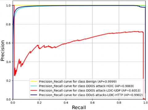
The dataset under investigation is acknowledged for its significant imbalance, characterized by a predominant "Benign" class, representing 85.95% of the examples, and a notably minuscule "DDOS attack-LOIC-UDP" class, constituting a mere 0.02%. Classes such as "DDOS attack-HOIC" and "DDoS attacks-LOIC-HTTP" are also observed to have substantially lower representation in comparison to the majority class. In response to this imbalance, performance metrics that are adept at handling skewed datasets have been employed. These include the area under the Receiver Operating Characteristic (ROC) curve, the average precision derived from the precision-recall curve with the parameter “average” set to “macro” for both curves, BA, the macro_F1-score, and the MCC. Each of these metrics has been carefully selected for their capacity to provide a more nuanced and balanced evaluation of the model’s performance, taking into consideration the inherent imbalance of the dataset.
Figure 1 delineates the architectural framework propounded in the present research endeavor. This framework encompasses four sequential stages, meticulously designed to ensure the integrity and effectiveness of the investigative process. In the first stage, dataset preprocessing is conducted, an integral component of which comprises the data cleansing phase. This is followed by normalization and scaling procedures, label encoding, and the meticulous selection of pertinent features. The dataset subsequently undergoes partitioning in the second stage, resulting in distinct subsets designated for training, validation, and testing purposes. The third stage is characterized by the implementation of BO, a sophisticated approach employed to refine and optimize the model’s hyperparameters. The culminating stage encompasses model training, utilizing the hyperparameters derived from the preceding BO. Model validation and evaluation are subsequently conducted, utilizing the test data and a comprehensive suite of performance metrics.
Figure 1. The architecture of the proposed approach
5.1 Dataset preprocessing
Upon the amalgamation of csv files constituting the CICIDS2018 DDOS attack dataset, the dataset was subjected to a pre-processing phase, a pivotal step in the preparation of data for application of ML and DL algorithms. This phase holds paramount importance, as it facilitates efficient learning from the available data, culminating in precise classifications.
Inconsistencies within columns of the dataset were addressed through deletion, ensuring the elimination of potential biases or adverse effects stemming from data of suboptimal quality. Values that were missing or infinite were managed with precision, the option was used to handle infinite values as nan "pd.set_option('mode.use_inf_as_na', True)", and then all rows containing nan (null value) were removed from our dataset.
Moreover, the dataset presented challenges due to disparate units of measurement and varying value ranges across different features. To counteract these challenges and ensure comparability across features, normalization and scaling were employed. The StandardScaler transformation from Scikit-learn was utilized, transforming the data such that each feature possessed a mean of zero and a variance of one [9]. The formula for this transformation, applied to each feature x, is expressed as:
${{x}_{St}}=\frac{(x-mean(x))}{std(x)}$ (7)
where $x_{S t}$ is the standardized value of feature x, mean(x) is the mean of the feature and std(x) is the standard deviation of the feature.
Regarding the treatment of categorical features, notably class labels, a transformation into numerical format is requisite for their assimilation by ML algorithms. The pre-processing phase commonly encompasses the deployment of encoding techniques to aptly represent these features. In the context of this study, classes from Scikit-learn, namely LabelEncoder and OneHotEncoder, were employed. The former was utilized for the XGBoost algorithm, while the latter served the RF and SGD algorithms.
5.1.1 Features selection
The pivotal role of feature selection in the ML pipeline is acknowledged, its primary aim being the discernment of the most pertinent features for a specified problem, whilst concurrently eliminating those deemed superfluous or redundant. A judicious execution of feature selection not only enhances the accuracy of model predictions but also mitigates model complexity and expedites the training procedure. The overarching goal of this process is the reduction of data dimensionality, a reduction achieved without compromising, and potentially even augmenting, the performance of the model.
In this study, the "feature importance" methodology of XGBoost was employed as the principal mechanism for feature selection, guiding the inclusion or exclusion of features in the training of models. This approach computes the importance of each feature based on its contribution to the amelioration of model error in the construction of DTs, subsequently assigning an importance score to each feature.
An XGBoost model was trained utilizing the CIC-IDS2018 DDOS attack dataset, and the resultant feature importance scores were visualized and arranged in descending order. Figure 2 delineates the salient features of the CIC-IDS2018 DDOS attack dataset as discerned by the deployed XGBoost algorithm, presented in the form of a horizontal bar chart.
The selection of the most pertinent features was conducted with a focus on retaining only those with an importance surpassing a specified threshold k, while disregarding features of lesser significance. To achieve this objective, an experimental procedure was undertaken, entailing the following steps:
Initially, the threshold was set to $k_1>0.0001$, resulting in 29 features meeting the established criterion. Subsequently, the threshold was adjusted to $k_2>0.001$, yielding 20 features in accordance with the stipulated requirement. Post the removal of features deemed irrelevant based on each threshold, the modified datasets were subjected to evaluation employing the RF, XGBoost, and SGD algorithms. The performance of each algorithm was assessed in terms of accuracy and the macro-average F1-score.
Figure 2. Feature importance graph by XGBoost algorithm
The macro-average F1-score was selected as the evaluation metric, acknowledging the imbalanced nature of the CICIDS2018 DDOS attack dataset. Within the multi-class context, this metric is computed by first determining the F1-score for each individual class, followed by calculating the average of these scores. This approach ensures a balanced evaluation of model performance, attributing equal weight to each class irrespective of their prevalence or disparity.
Table 3. Thresholds for selecting the most relevant features
|
Threshold |
Models |
Accuracy |
Macro Avg F1 Score |
|
K1>0.0001 |
RF |
1 |
0.98 |
|
K1>0.0001 |
XGBoost |
1 |
0.98 |
|
K1>0.0001 |
SGD |
0.88 |
0.55 |
|
K2>0.001 |
RF |
1 |
0.98 |
|
K2>0.001 |
XGBoost |
1 |
0.98 |
|
K2>0.001 |
SGD |
0.95 |
0.83 |
Upon analysis of the results, it was observed that both the RF and XGBoost algorithms exhibited consistent performance across the two threshold settings, achieving an accuracy of 1 and a macro-average F1-score of 0.98. In contrast, the SGD algorithm demonstrated variation in performance between the two thresholds. Specifically, the evaluation metrics associated with threshold $k_1>0.0001$ were notably lower in comparison to those recorded for threshold $k_2>0.001$. These findings are comprehensively presented in Table 3 .
Based on aforementioned results, the decision was made to retain features surpassing the threshold of $k_2>0.001$, resulting in a shortlist of the top 20 most pertinent features. These selected features are meticulously detailed in Table 4, wherein each entry delineates the sequential position of the feature within the initial dataset, alongside its respective nomenclature, data typology, and corresponding importance score.
Table 4. Features selected by the XGBoost method from the CIC-IDS2018 DDOS attacks dataset
|
Feature Number |
Feature |
Data Type |
Feature Importance Score |
|
16 |
Bwd Pkt Len Std |
float64 |
0.436436 |
|
7 |
TotLen Fwd Pkts |
float64 |
0.187275 |
|
1 |
Dst Port |
int64 |
0.157668 |
|
68 |
Init Fwd Win Byt |
int64 |
0.057977 |
|
22 |
Flow IAT Min |
float64 |
0.034996 |
|
23 |
Fwd IAT Tot |
float64 |
0.033091 |
|
49 |
PSH Flag Cnt |
int64 |
0.016368 |
|
50 |
ACK Flag Cnt |
int64 |
0.014257 |
|
18 |
Flow Pkts/s |
float64 |
0.012913 |
|
5 |
Tot Fwd Pkts |
int64 |
0.009571 |
|
4 |
Flow Duration |
int64 |
0.006550 |
|
21 |
Flow IAT Max |
float64 |
0.006274 |
|
25 |
Fwd IAT Std |
float64 |
0.004876 |
|
32 |
Bwd IAT Min |
float64 |
0.004392 |
|
76 |
Idle Mean |
float64 |
0.003806 |
|
11 |
Fwd Pkt Len Mean |
float64 |
0.003112 |
|
70 |
Fwd Act Data Pkt |
int64 |
0.002539 |
|
12 |
Fwd Pkt Len Std |
float64 |
0.001815 |
|
78 |
Idle Max |
float64 |
0.001683 |
|
51 |
URG Flag Cnt |
int64 |
0.001462 |
Utilizing the XGBoost algorithm, a selection of features has been meticulously identified, demonstrating substantial relevance in augmenting the performance of the anomaly-based intrusion detection model. This is achieved through the discernment of atypical patterns and behaviors within network traffic.
The feature 'Bwd Pkt Len Std' is particularly noteworthy, as it encapsulates the variability in the size of backward direction packets. This is crucial in the context of Denial of Service (DDoS) attacks, which are known to precipitate pronounced alterations in the distribution of packet sizes, thereby serving as a potential hallmark of malicious activity.
'TotLen Fwd Pkts' emerges as another significant feature, providing utility in the identification of DDoS attacks characterized by the transmission of substantial forward packets aimed at overwhelming the target. Concurrently, 'Dst Port', the feature denoting the destination port, plays a vital role in pinpointing attacks meticulously crafted to compromise specific services.
The feature 'Init Fwd Win Byt', representing the initiation of sending windows, is deemed pertinent for the detection of incipient attacks attempting to forge malicious connections through the manipulation of sending windows. Furthermore, 'Flow IAT Min' quantifies the minimum inter-arrival time between consecutive data flows, with DDoS attacks having the potential to disrupt standard traffic patterns, manifesting in anomalously low values.
'Fwd IAT Tot' offers insights into the temporal intervals between forward packets, where abrupt variations may be indicative of traffic anomalies. 'PSH Flag Cnt' and 'ACK Flag Cnt' are instrumental in identifying urgent packet transmissions and tracking the prevalence of ACK packets, respectively, both of which are tactics frequently exploited in amplified reflection attacks.
Additional features such as 'Flow Pkts/s', 'Tot Fwd Pkts', 'Flow Duration', 'Flow IAT Max', 'Fwd IAT Std', 'Bwd IAT Min', 'Idle Mean', 'Idle Max', 'Fwd Pkt Len Mean', 'Fwd Act Data Pkt', 'Fwd Pkt Len Std', and 'URG Flag Cnt' are elaborated upon, underscoring their integral roles in the holistic detection of network irregularities and potential security breaches.
In essence, through vigilant monitoring of these pivotal aspects of network traffic, the model is adeptly equipped to not only identify but also counteract malicious activities, thereby substantially fortifying the integrity of network security.
The next step is to divide the processed data set into a training data set comprising 70% of the data, a validation data set with 18% and a test data set with 12%.
5.2 BO
In the pursuit of advancing the capabilities of IDS, particularly in relation to DDoS attacks, this research endeavors to enhance the efficacy of three preeminent algorithms extensively applied in the realm of ML: XGBoost, RF, and SGD.
Acknowledging the prevalence of numerous hyperparameters within ML algorithms, necessitating meticulous tuning to attain optimal results, BO has been employed in this study. This method facilitates the identification of superior hyperparameter values, with the objective of maximizing a designated performance metric. Consequently, this approach endeavors to yield enhanced model performance while concurrently economizing on time, presenting a preferable alternative to exhaustive search methodologies such as GS and random search.
Within the framework of this study, a specific search space has been delineated for each algorithm, encapsulating a spectrum of potential values for the hyperparameters subject to optimization. The hyperparameters subjected to examination encompass: for XGBoost, max_depth, learning_rate, min_child_weight, gamma, reg_alpha, reg_lambda, and n_estimators; for RF, n_estimators, criterion, max_depth, and max_features; and for SGD, loss, alpha, penalty, and max_iter. Table 5 elucidates the defined search spaces and explicates the significance of each hyperparameter.
For the purpose of the objective function, two distinct performance metrics were evaluated: average_precision_score and Roc_auc_score, both employing the Average='macro' parameter. The rationale behind optimizing these particular metrics stems from their relevance in IDS, where it is imperative to accurately identify attacks while minimizing the rate of FP. This necessitates a balanced trade-off between precision and recall, as well as between the rates of FP and FN. The metric average_precision quantitatively assesses the model’s precision, evaluating its capacity to accurately classify positive instances (intrusions) among those predicted as positive. Conversely, the metric Roc_auc_score serves as a comprehensive indicator of the model’s overall performance. The selection of these metrics is strategically aimed at identifying the optimal hyperparameters for each algorithm under investigation, with the objective of maximizing the values of these objective functions.
The precision-recall curve is delineated, representing precision P(r) as a function of recall r. The Average Precision (AP) computes the mean value of P(r) over the interval r=0 to r=1 [38]. Derived from the prediction scores, AP encapsulates the precision-recall curve, presenting it as a weighted average of the precisions computed at each respective threshold. The increment in recall from the preceding threshold serves as the weight in this calculation [39]:
$\text{AP}=\sum\limits_{n}{\left( {{R}_{n}}-{{R}_{n-1}} \right)}{{P}_{n}}$ (8)
where $P_n$ and $R_n$ are precision and recall at the $\mathrm{n}$-th threshold.
The metric average_precision_score has been selected, with the specification "average='macro'" implemented for this evaluation. Within a multi-class context, the AP is computed as the arithmetic mean of the average precision scores allocated to each distinct class [40]. It is important to highlight that this approach does not account for any potential imbalance in label distribution [39].
Consequently, the average_precision_score serves as a metric that determines the weighted average of precisions attained at various thresholds for each class individually, while also considering the actual distribution of classes present within the data. This metric comprehensively incorporates both precision and recall for every individual class, thereby offering a holistic insight into the model's performance capabilities.
In relation to the second objective function scrutinized in this research, the Roc_auc_score function, also recognized as ROC (Receiver Operating Characteristic) AUC (Area Under Curve) or AUROC (Area Under the Receiver Operating Characteristic Curve), is employed to calculate the area beneath the ROC curve, based on the prediction scores [41].
The ROC curve itself is a graphical representation, delineating the performance of a binary classification system across all possible classification thresholds [42]. This curve plots the True Positive Rate (TPR) against the False Positive Rate (FPR), spanning various threshold values. The TPR is represented along the Y-axis, while the FPR is plotted on the X-axis. The optimal point on this curve would correspond to a FPR of zero coupled with a TPR of one. The overarching objective is to simultaneously maximize the TPR and minimize the FPR. Generally, a larger AUC is indicative of superior model performance [43].
ROC curves are predominantly utilized in the realm of binary classification, facilitating the distinct definition of the TPR and FPR. When venturing into the domain of multi-class classification, a clear delineation of TPR or FPR necessitates the binarization of the output, a process executable through two predominant schemes: the Un-vs-Un scheme, which engages in a pairwise comparison of each unique class combination, and the Un-vs-Rest scheme, which entails comparing each individual class against all remaining classes [43].
In the context of this research endeavor, the multi-class One-vs-Rest (OvR) strategy, alternatively known as One-vs-All, was employed. This strategy necessitates the computation of an ROC curve for each class within the n_classes. In each iteration, a specific class is designated as the positive class, while the aggregate of other classes is treated as a singular negative class [43].
To address and mitigate the issue of class imbalance and ensure equitable treatment across all classes, the 'macro' option was selected for the Average parameter of the Roc_auc_score metric. This entails the computation of the arithmetic mean of the metric independently for each class.
In the iterative optimization process, a maximum number of iterations was established for each algorithm under study, pertaining to both Roc_auc_score and Average_precision_score objective functions. Upon completion of this iterative loop, the optimal value and corresponding hyperparameters, yielding the most proficient performance, were ascertained for each objective function. Specifically, the maximum iterations were set at 15 for the RF algorithm, 18 for the XGBoost algorithm, and three distinct values—15, 20, and 30—were evaluated for the SGD algorithm. The subsequent section, Table 6, delineates the optimal hyperparameters derived from each objective function for each algorithm, while Table 7 enumerates the associated processing times.
Subsequent to the BO, the algorithms under investigation - RF, XGBoost, and SGD—were subjected to both the optimized hyperparameters and their default settings. The rationale for this dual approach was to establish a baseline for performance comparison, particularly in the context of DDOS attack detection systems.
The selection of classifiers - XGBoost, RF, and SGD Classifiers - was predicated on their distinctive attributes, which aligned with the research objectives pertaining to precision, speed, robustness, and capacity to manage extensive data sets. XGBoost, a boosting model, was chosen for its prowess in delivering high accuracy, execution speed, and resilience against overfitting, rendering it an exemplary choice for anomaly-based intrusion detection. RF, an ensemble model, is lauded for its precision, resistance to overfitting, and aptitude for handling diverse data types, which are imperative in intrusion detection scenarios. Lastly, the SGD classifier, grounded in SGD, was selected for its efficiency in processing large volumes of data and its expedited computational capabilities, both of which are quintessential in IT security contexts.
Table 5. Defined search space for the 3 algorithms studied
|
Models |
Defined Search Space |
|
|
space = [Categorical([3,5,6], name="max_depth"), |
|
|
Categorical([0.01, 0.05, 0.1, 0.15, 0.20, 0.25, 0.3], name="learning_rate"), |
|
|
Categorical([1,5,7,10], name="min_child_weight"), |
|
XGBoost |
Categorical([0, 0.1, 0.2, 0.3, 0.5, 1], name= "gamma"), |
|
|
Categorical([0, 0.0001, 0.01, 0.1, 0.5, 1], name="reg_alpha"), |
|
|
Categorical([0, 0.0001, 0.01, 0.1, 0.5, 1], name="reg_lambda"), |
|
|
Categorical([50,80], name="n_estimators")] |
|
|
space = [Categorical([50,80,100,110], name="n_estimators"), |
|
|
Categorical(["gini", "entropy", "log_loss"], name="criterion"), |
|
RF |
Categorical([3,5,6, None], name="max_depth"), |
|
|
Categorical(["sqrt", "log2", None], name="max_features")] |
|
|
space = [Categorical(["hinge", "log_loss", "modified_huber", "perceptron"], name="loss"), |
|
SGD |
Categorical([0.0001, 0.001, 0.01, 0.1], name="alpha"), |
|
|
Categorical(['l2', 'l1', 'elasticnet', None], name= "penalty"), |
|
|
Categorical([1000,3000, 5000, 10000], name="max_iter")] |
Table 6. BO result
|
Models |
Nb_Calls |
Best HyperParameters (AP) |
Best (AP) |
Best HyperParameters (AUC) |
Best (AUC) |
|
SGD |
15 |
{'loss': 'perceptron', 'alpha': 0.001, 'penalty': 'l2', 'max_iter': 10000} |
0.8943 |
{'loss': 'perceptron', 'alpha': 0.0001, 'penalty': 'elasticnet', 'max_iter': 1000} |
0.9993 |
|
SGD |
20 |
{'loss': 'perceptron', 'alpha': 0.0001, 'penalty': 'l2', 'max_iter': 10000} |
0.8954 |
{'loss': 'perceptron', 'alpha': 0.001, 'penalty': 'l2', 'max_iter': 5000} |
0.9994 |
|
SGD |
30 |
{'loss': 'hinge', 'alpha': 0.0001, 'penalty': 'l1', 'max_iter': 5000} |
0.8908 |
{'loss': 'perceptron', 'alpha': 0.0001, 'penalty': 'l2', 'max_iter': 3000} |
0.9995 |
|
RF |
15 |
{ n_estimators=100; criterion= entropy; max_depth= None; max_features= None} |
0.9948 |
{ n_estimators= 110; criterion= entropy; max_depth= None; max_features= log2 } |
1.0000 |
|
XGBoost |
18 |
{ max_depth =3; learning_rate= 0,3; min_child_weight = 5; gamma= 0; reg_alpha= 0,1; reg_lambda= 0,01; n_estimators= 80 } |
0.9967 |
{max_depth=6; learning_rate= 0,2; min_child_weight= 5; gamma= 0,2; reg_alpha= 0; reg_lambda= 0,1; n_estimators= 80 } |
1.0000 |
Table 7. BO runtime
|
Model |
Nb_Calls |
Learning_Period(s) |
Predictive_Period (s) |
Total Learning and Predictive Period (s) |
|
SGD_AP |
30 |
2445.785 |
16.723 |
2462.507 |
|
SGD_AUC |
30 |
1939.482 |
16.875 |
1956.356 |
|
RF_AP |
15 |
29965.195 |
452.254 |
30417.449 |
|
RF_AUC |
15 |
64317.759 |
417.664 |
64735.423 |
|
XGB_AP |
18 |
41472.845 |
62.795 |
41535.640 |
|
XGB_AUC |
18 |
43787.210 |
65.340 |
43852.550 |
In scenarios involving imbalanced datasets, the evaluation methodology for the performance of multi-class classification models encompassed a twofold approach. Initially, a holistic assessment was conducted using global metrics - Accuracy, BA, MCC, and macro_F1_score - to provide a comprehensive view of the algorithms' efficacy. Subsequently, a more granular analysis was undertaken, examining individual class performances based on Precision, Recall, F1-score, FPR, and the Precision-Recall Curve, complemented by the AP Score. The final facet of evaluation pertained to the execution times of each model, ensuring a thorough appraisal of their performance.
6.1 Hardware and environment setting
The experiments delineated in this manuscript were executed on the Google Colab Pro+ platform, a derivative of Google Research. This platform provides a hosted Jupyter notebook service, obviating the necessity for configuration, and is endowed with 54.8 gigabytes of high RAM for computational tasks. The construction, training, evaluation, and testing of the ML models were carried out within the Scikit-Learn framework, an open-source Python library renowned for its simplicity and efficacy, drawing upon the capabilities of the NumPy, SciPy, and matplotlib libraries. For the implementation of XGBoost, the xgboost Python module was integrated into the Scikit-Learn framework, serving dual functions as a data selection tool and ML algorithm. Sequential model-based optimization, requisite for BO, was facilitated through the employment of the scikit-optimize module, an open-source tool built upon NumPy, SciPy, and Scikit-Learn. The construction of the models was undertaken using Jupyter Notebook, with Python as the programming language of choice. Data cleaning and feature selection were conducted utilizing the Pandas and NumPy frameworks, while data visualization was achieved through Matplotlib and the Seaborn framework. BO was conducted via Scikit-optimize, and Scikit-learn was employed for comprehensive data analysis.
6.2 Performance metrics
The evaluation of classification model performance within this study hinges on the mathematical computation of various metrics, each rooted in the distinct permutations of elements within the confusion matrix: True Positives (TP), True Negatives (TN), False Positives (FP), and False Negatives (FN). Herein, TP denote instances wherein the model accurately identifies the positive class, whereas TN pertain to cases of correct negative class prediction. Conversely, FP-categorized as Type I errors-occur when the model erroneously predicts the positive class in lieu of the negative class. FN, or Type II errors, arise when the model inaccurately predicts the negative class, despite the true classification being positive.
Accuracy serves as a pivotal metric within this framework, quantifying the overall precision of the classification model. It is calculated as the proportion of accurately predicted instances (encompassing both TPs and TNs) relative to the aggregate number of instances present in the dataset.
$Accuracy =\frac{T P+T N}{F P+F N+T P+T N}$ (9)
BA is a metric judiciously employed in the context of imbalanced datasets, accommodating for disparities in class distribution. By computing the average recall, or TP rate, across each individual class, BA offers a nuanced and more precise portrayal of a model’s performance, particularly in scenarios characterized by imbalanced classes.
$BA=\frac{(\text{ }Sensitivity\text{ }+\text{ }Specificity\text{ })}{2}$ (10)
where,
$\begin{align} & Sensitivity\text{ }(Recall\text{ })=\frac{TP}{TP+FN} \\ & Specificity\text{ }=\frac{TN}{TN+FP} \\\end{align}$
MCC serves as a comprehensive metric for evaluating the performance of binary classification models, encapsulating all four components of the confusion matrix: TPs, TNs, FPs, and FNs. It effectively quantifies the correlation between the observed and predicted classifications, with its values spanning from -1, indicative of completely discordant predictions, to +1, denoting flawless prediction accuracy. A score of 0 from MCC implies that the model's predictions are no better than random chance.
$MCC=\frac{(TP*TN-FP*FN)}{\sqrt{\left( \begin{align} & (TP+FP)*(TP+FN) \\ & *(TN+FP)*(TN+FN) \\\end{align} \right)}}$ (11)
Recall measures the model's ability to correctly identify all positive instances (TPs) out of all actual positives. It is also known as the TP rate or sensitivity.
$Recall=\frac{TP}{TP+FN}$ (12)
Precision measures the model's ability to correctly predict positive instances (TPs) out of all instances predicted as positive. It assesses the reliability of positive predictions.
$Precision=\frac{TP}{TP+FP}$ (13)
The F1-score is the harmonic mean of precision and recall. It provides a single metric that balances both precision and recall, making it useful for assessing overall classification performance.
$f1-score=\frac{2*(Precision*Recall)}{(Precision+Recall)}$ (14)
The macro F1-score is the average F1-score calculated separately for each class and then averaged. It measures the balance between precision and recall across multiple classes in a classification problem.
$MacroF1-score=\frac{\sum\limits_{i=1}^{N}{F}1-\text{ }score{{\text{ }}_{i}}}{N}$ (15)
The FPR is the ratio of FP predictions to all actual negatives. It measures the model's ability to correctly classify negative instances.
$FPR=\frac{FP}{FP+TN}$ (16)
6.3 Implements, results and discussion
Subsequent to the completion of the data pre-processing phase, the derived dataset was partitioned into distinct subsets, with 70% allocated for training (training set), 18% for validation (validation set), and 12% for testing (test set). The application of BO yielded the results delineated in Table 6, encompassing the outcomes for all three investigated algorithms across the two objective functions: Average_precision_score and Roc_auc_score.
Regarding the SGD model, the decision was made to adopt the hyperparameters corresponding to the most elevated value attained between AP and AUC. In this instance, a notable AP of 0.8954 was achieved at the testing phase, corresponding to a BO iteration count (nb_calls) of 20. In contrast, the AUC value peaked at 0.995, associated with an nb_calls value of 30. It is imperative to underscore that the nb_calls parameter serves as the termination criterion for the iterative loop within the BO process. A meticulous examination of the results for the SGD model divulged a recurring presence of the hyperparameter “loss='perceptron'”, featured in five out of the six documented outcomes. Furthermore, the hyperparameters "alpha=0.0001" and "penalty=l2" manifested in four out of the six cases.
Turning attention to the RF and XGBoost algorithms, it was observed that the BO computational duration for both objective functions was considerably extensive, as elucidated in Table 7. The Colab Pro+ platform, serving as the computational environment for the experiments, enforces a continuous execution limit of 24 hours, beyond which all processing activities are curtailed. This operational constraint necessitated the selection of specific iteration numbers for these two models. Despite this limitation, both algorithms demonstrated exemplary performance, achieving an AUC of 1 and exhibiting remarkably high PA values, with XGBoost marginally outperforming RF in terms of the PA metric.
Following the application of BO, we proceeded to train, validate, and test the three algorithms under study. The aggregated results from the evaluation of the SGD, RF, and XGB models, utilizing both the optimal hyperparameters derived from BO and the default settings of the models, are displayed in Table 8.
Table 8. Result of the global evaluation of the SGD, RF and XGB algorithm
|
Algorithm |
Hyperparameter Basis |
Model |
Accuracy |
Balanced_Accuracy |
MCC |
Macro_F1_Score |
|
SGD |
macro_ap |
M1_Model= SGDClassifier (loss='perceptron'; alpha=0,0001; penalty=l2; max_iter=10000) |
0.997851 |
0.866470 |
0.991598 |
0.879416 |
|
SGD |
macro_roc_auc |
M2_Model= SGDClassifier (loss='perceptron'; alpha=0,0001; penalty=l2; max_iter=3000) |
0.997850 |
0.844379 |
0.991594 |
0.861148 |
|
SGD |
default hyperparameters |
M3_Model =SGDClassifier (loss='hinge'; alpha=0,0001; penalty=l2; max_iter=1000) |
0.989745 |
0.871967 |
0.959750 |
0.880472 |
|
RF |
macro_ap |
M4_Model= RandomForestClassifier (n_estimators= 100; criterion= ' entropy';max_depth =None; max_features= None) |
0.999959 |
0.966789 |
0.999838 |
0.972300 |
|
RF |
macro_roc_auc |
M5_Model= RandomForestClassifier (n_estimators= 110; criterion= ' entropy';max_depth =None; max_features= ' log2 ') |
0.999956 |
0.973656 |
0.999827 |
0.968834 |
|
RF |
default hyperparameters |
M6_Model= RandomForestClassifier (n_estimators= 100; criterion= ' gini';max_depth =None; max_features= ' sqrt ') |
0.999944 |
0.969503 |
0.999779 |
0.965338 |
|
XGB |
macro_ap |
M7_Model=XGBClassifier (max_depth=3; learning_rate= 0,3; min_child_weight= 5; gamma = 0; reg_alpha= 0,1; reg_lambda = 0,01; n_estimators = 80) |
0.999963 |
0.990906 |
0.999853 |
0.976434 |
|
XGB |
macro_roc_auc |
M8_Model=XGBClassifier( max_depth=6; learning_rate= 0,2; min_child_weight= 5; gamma = 0,2; reg_alpha= 0; reg_lambda = 0,1; n_estimators = 80) |
0.999969 |
0.992210 |
0.999878 |
0.980428 |
|
XGB |
Default Hyperparameters |
M9_Model=XGBClassifier( max_depth=3; learning_rate= 0,1; min_child_weight= 1; gamma = 0; reg_alpha= 0; reg_lambda = 1; n_estimators = 100) |
0.999924 |
0.989490 |
0.999698 |
0.971938 |
Table 9. Precision, recall and f1_score results for SGD, RF and XGB models for individual classes
|
Precision_test |
M1_SGD |
M2_SGD |
M3_SGD |
M4_RF |
M5_RF |
M6_RF |
M7_XGB |
M8_XGB |
M9_XGB |
|
Benign |
99.99% |
99.99% |
99.48% |
100.00% |
100.00% |
100.00% |
100.00% |
100.00% |
100.00% |
|
DDOS attack-HOIC |
99.35% |
99.38% |
94.53% |
100.00% |
100.00% |
100.00% |
100.00% |
100.00% |
100.00% |
|
DDOS attack-LOIC-UDP |
62.04% |
58.47% |
64.56% |
91.28% |
85.71% |
84.57% |
85.45% |
87.91% |
82.74% |
|
DDoS attacks-LOIC-HTTP |
97.67% |
97.64% |
97.85% |
99.96% |
99.97% |
99.96% |
99.99% |
99.99% |
99,98% |
|
Recall_test |
M1_SGD |
M2_SGD |
M3_SGD |
M4_RF |
M5_RF |
M6_RF |
M7_XGB |
M8_XGB |
M9_XGB |
|
Benign |
99.77% |
99.77% |
99.34% |
100.00% |
100.00% |
100.00% |
100.00% |
100.00% |
100.00% |
|
DDOS attack-HOIC |
99.95% |
99.94% |
99.98% |
100.00% |
100.00% |
100.00% |
100.00% |
100.00% |
100.00% |
|
DDOS attack-LOIC-UDP |
46.96% |
38.12% |
56.35% |
86.74% |
89.50% |
87.85% |
96.41% |
96.92% |
95.90% |
|
DDoS attacks-LOIC-HTTP |
99.90% |
99.91% |
93.12% |
99.98% |
99.96% |
99.96% |
99.95% |
99.96% |
99.90% |
|
f1_score_test |
M1_SGD |
M2_SGD |
M3_SGD |
M4_RF |
M5_RF |
M6_RF |
M7_XGB |
M8_XGB |
M9_XGB |
|
Benign |
99.88% |
99.88% |
99.41% |
100.00% |
100.00% |
100.00% |
100.00% |
100.00% |
100.00% |
|
DDOS attack-HOIC |
99.65% |
99.66% |
97.18% |
100.00% |
100.00% |
100.00% |
100.00% |
100.00% |
100.00% |
|
DDOS attack-LOIC-UDP |
53.46% |
46.15% |
60.18% |
88.95% |
87.57% |
86.18% |
90.60% |
92.20% |
88.84% |
|
DDoS attacks-LOIC-HTTP |
98.78% |
98.76% |
95.42% |
99.97% |
99.97% |
99.96% |
99.97% |
99.98% |
99.94% |
These results offer a comprehensive insight into the performance of the three algorithms in identifying DDOS attack intrusions within the CICIDS2018 dataset, showcasing an overall commendable performance.
Focusing on Accuracy, a metric that reflects a model's proficiency in accurately predicting the predominant class, we arranged the results yielded by the various models in a descending order based on this metric. This exercise resulted in the following hierarchy: M8_XGB>M7_XGB>M4_RF> M5_RF>M6_RF>M9_XGB>M1_SGD>M2_SGD>M3_SGD, with corresponding accuracy values of 0.999969, 0.999963, 0.999959, 0.999956, 0.999944, 0.999924, 0.997851, 0.997850, and 0.989745, respectively.
In the conducted study, three classifier models, namely SGD, RF, and XGBoost (XGB), were scrutinized through the lens of BO, with their performances meticulously evaluated and ranked based on various metrics. Observations were made regarding the superior performance exhibited by the XGBoost classifier models M8_XGB and M7_XGB, both outcomes of BO. These models demonstrated exceptional efficacy, surpassing their counterparts in the RF and SGD classifier domains. Notably, the default classifier values of RF and XGBoost, as represented by models M6_RF and M9_XGB, showcased commendable performance, outstripping all SGD classifier models.
Focusing on BA, a critical metric for gauging a model's discriminative capabilities across diverse classes whilst accounting for potential class imbalances, the XGBoost optimized models were identified as the front runners. The ensuing ranking, delineated as M8_XGB>M7_XGB> M9_XGB>M5_RF>M6_RF>M4_RF>M3_SGD>M1_SGD> M2_SGD, with corresponding values 0.992210>0.990906> 0.989490>0.973656>0.969503>0.966789>0.871967>0.866470>0.844379, highlighted the lower positioning of SGD models. Intriguingly, the M3_SGD model, adhering to the classifier's default hyperparameters, outperformed the algorithm's optimized counterparts.
In terms of the MCC, a robust metric providing a holistic assessment of model performance, particularly in scenarios characterized by class imbalances, the optimized XGBoost models once again asserted their dominance. They were closely followed by the optimized models from the RF ensemble. The rankings, as deduced, were as follows: M8_XGB>M7_XGB>M4_RF>M5_RF>M6_RF>M9_XGB>M1_SGD>M2_SGD>M3_SGD, with corresponding MCC values of 0.999878>0.999853>0.999838>0.999827>0.999779>0.999698>0.991598>0.991594>0.959750. It was discerned that models operating under default parameter settings (M9_XGB, M6_RF, and M3_SGD) were outpaced by their optimized counterparts across each algorithm.
The Macro F1-score, serving as a critical indicator of the harmonic balance between precision and recall across various classes, was meticulously examined for different models. The ensuing analysis yielded a hierarchical ranking as follows: M8_XGB>M7_XGB>M4_RF>M9_XGB>M5_RF>M6_RF> M3_SGD>M1_SGD>M2_SGD, with corresponding values being 0.980428, 0.976434, 0.972300, 0.971938, 0.968834, 0.965338, 0.880472, 0.879416, and 0.861148, respectively. Notably, the models affiliated with the SGD classifier were positioned at the lower end of the spectrum.
In an exhaustive evaluation across all four metrics, the XGBoost model M8_XGB, parameterized as XGBClassifier (max_depth=6; learning_rate=0.2; min_child_weight=5; gamma=0.2; reg_alpha=0; reg_lambda=0.1; n_estimators=80), consistently emerged as the top performer. When delving into a comparative analysis of the optimized models versus those operating under default values for each algorithm, discerning observations were made. Within the XGBoost realm, models M8_XGB and M7_XGB exhibited superior performance across all metrics in comparison to M9_XGB. In the context of the RF ensemble, models M4_RF and M5_RF outperformed M6_RF in a majority of metrics, with the exception of BA where M4_RF lagged slightly behind M6_RF. On the SGD front, models M1_SGD and M2_SGD demonstrated prowess in Accuracy and MCC, surpassing M3_SGD. However, they fell short in BA and Macro F1-score when juxtaposed with M3_SGD.
Table 9 offers a granular view, encapsulating the precision, recall, and F1-score metrics, as garnered by the models in relation to the individual classes encompassed within the CICIDS2018 DDOS attack dataset.
At this stage, it is observed that all models pertaining to the RF and XGBoost algorithms exhibit impeccable performance, achieving a 100% detection and prediction rate for the "Benign" and "DDOS-attack-HOIC" classes. In contrast, the SGD classifier models present a more nuanced performance landscape.
Specifically, for the "Benign" class, the M3_SGD model is outperformed by both M1_SGD and M2_SGD across all three evaluation metrics. In the case of the "DDOS-attack-HOIC" class, the M3_SGD model once again lags behind, particularly in terms of accuracy and F1 score, rendering M1_SGD and M2_SGD as more proficient for this specific class.
When attention is shifted to the "DDOS-attack-LOIC-UDP" class, the F1 score reveals that the M8_XGB model excels with a commendable score of 92.20%, while M2_SGD is situated at the lower end of the spectrum with a score of 46.15%. In terms of the "DDOS-attack-LOIC-HTTP" class, the M8_XGB model maintains its superior stance, achieving an impressive score of 99.98%, whereas M3_XGB is identified as the underperformer with a score of 95.42%.
These findings facilitate a comprehensive ranking of the RF and XGBoost models based on their precision, recall, and F1 score metrics, from the highest to the lowest performing. However, the classification of models within the SGD algorithm remains ambiguous. It is, nonetheless, definitively established that M1_SGD and M2_SGD outshine M3_SGD in the "Benign," "DDOS-attack-HOIC," and "DDOS-attack-LOIC-HTTP" classes. Conversely, M3_SGD demonstrates superiority over M1_SGD and M2_SGD in the "DDOS-attack-LOIC-UDP" class, culminating in the conclusion that M1_SGD is the overall superior model within the SGD family.
Comparatively, models under the SGD algorithm are observed to perform suboptimally relative to their XGBoost and RF counterparts. Consequently, the performance hierarchy from the most to least effective is established as follows: M8_XGB > M7_XGB > M4_RF > M9_XGB > M5_RF > M6_RF > SGD models.
Figure 3. Precision_recall curves for SGD models
Table 10. The results of the FPR
|
|
M1_SGD |
M2_SGD |
M3_SGD |
M4_RF |
M5_RF |
M6_RF |
M7_XGB |
M8_XGB |
M9_XGB |
|
Benign |
3,81E-04 |
4,01E-04 |
3,12E-02 |
1,31E-05 |
6,57E-06 |
6,57E-06 |
6,59E-06 |
6,59E-06 |
2,04E-04 |
|
DDOS attack-HOIC |
5,46E-04 |
5,22E-04 |
4,82E-03 |
0,00E+00 |
0,00E+00 |
0,00E+00 |
0,00E+00 |
0,00E+00 |
1,01E-06 |
|
DDOS attack-LOIC-UDP |
4,85E-05 |
4,57E-05 |
5,22E-05 |
1,40E-05 |
2,52E-05 |
2,70E-05 |
2,98E-05 |
2,42E-05 |
3,64E-05 |
|
DDoS attacks-LOIC-HTTP |
1,65E-03 |
1,67E-03 |
1,42E-03 |
2,69E-05 |
1,89E-05 |
2,99E-05 |
6,98E-06 |
5,98E-06 |
1,10E-05 |
Table 11. Runtimes undertaken by the SGD, RF and XGBoost algorithms
|
Model |
Learning_Period (Seconds) |
Validation_Predictive_Period (Seconds) |
Test_Predictive_Period (Seconds) |
Total Execution Time (Seconds) |
|
M1_SGD= SGDClassifier( loss='perceptron'; alpha=0,0001; penalty=l2; max_iter=10000) |
45.884 |
0.336 |
0.168 |
46.387 |
|
M2_SGD= SGDClassifier( loss='perceptron'; alpha=0,0001; penalty=l2; max_iter=3000) |
47.989 |
0.389 |
0.176 |
48.554 |
|
M3_SGD =SGDClassifier( loss='hinge'; alpha=0,0001; penalty=l2; max_iter=1000) |
44.423 |
0.250 |
0.172 |
44.845 |
|
M4_RF= RandomForestClassifier( n_estimators= 100; criterion= ' entropy';max_depth =None; max_features= None) |
4282.952 |
11.113 |
7.404 |
4301.468 |
|
M5_RF= RandomForestClassifier( n_estimators= 110; criterion= ' entropy';max_depth =None; max_features= ' log2 ') |
1641.709 |
14.140 |
9.280 |
1665.129 |
|
M6_RF= RandomForestClassifier( n_estimators= 100; criterion= ' gini';max_depth =None; max_features= ' sqrt ') |
1231.130 |
12.946 |
8.642 |
1252.718 |
|
M7_XGB=XGBClassifier( max_depth=3; learning_rate= 0,3; min_child_weight= 5; gamma = 0; reg_alpha= 0,1; reg_lambda = 0,01; n_estimators = 80) |
538.529 |
0.660 |
0.450 |
539.638 |
|
M8_XGB=XGBClassifier( max_depth=6; learning_rate= 0,2; min_child_weight= 5; gamma = 0,2; reg_alpha= 0; reg_lambda = 0,1; n_estimators = 80) |
541.611 |
0.808 |
0.542 |
542.962 |
|
M9_XGB=XGBClassifier( max_depth=3; learning_rate= 0,1; min_child_weight= 1; gamma = 0; reg_alpha= 0; reg_lambda = 1; n_estimators = 100) |
681.492 |
0.792 |
0.526 |
682.810 |
To discern the relative performance of models within the SGD algorithm, the precision-recall curve, illustrating the trade-off between precision and recall across varying classification thresholds, was employed alongside the average precision metric for each class. The insights gleaned from the analysis of the precision-recall curves for SGD models are meticulously presented in Figure 3.
The graphical representations elucidated in these precision-recall curves corroborate the earlier findings, underscoring the inability of the three SGD models to accurately classify instances of the "DDOS-attack-LOIC-UDP" class. This observation is consistent with the previously delineated results derived from the class-specific recall and precision metrics.
In particular, the precision-recall curve for the M3_SGD model, when assessed in the context of the "DDOS-attack-HOIC" class, fails to ascend to the apex of precision, a feat achieved by its two counterparts. Additionally, the curve pertinent to the "DDOS-attack-LOIC-HTTP" class for the M3_SGD model reveals a decrement in precision concomitant with an increment in recall, further solidifying the model's position as the least efficacious among the SGD classifiers.
Conversely, the M1_SGD model distinguishes itself through superior performance, evidenced by the higher AP values across various classes when juxtaposed with the AP values of the other two SGD models. Consequently, the performance of these models can be hierarchically arranged as follows: M1_SGD > M2_SGD > M3_SGD, solidifying M1_SGD's standing as the most proficient model within the SGD algorithmic framework.
An examination of the FPR outcomes presented in Table 10 elucidates the comparative performance of various models, revealing discernible trends. The SGDClassifier models exhibit a markedly higher FPR across all classes when juxtaposed with their RF and XGBClassifier counterparts. Specifically, the M3_SGD model manifests exceedingly elevated FPR rates for both the Benign and DDOS-attack-HOIC classes. Conversely, the models M6_RF, M5_RF, M8_XGB, and M7_XGB are distinguished by their minimized FPR rates.
In the context of the DDOS-attack-HOIC class, it is noteworthy that the models M6_RF, M5_RF, M8_XGB, M7_XGB, and M4_RF achieved a perfect classification with zero FPs. As for the "DDOS-attack-LOIC-UDP" class, a low FPR was consistently maintained across all classifiers. With respect to the "DDoS-attacks-LOIC-HTTP" class, the models M8_XGB and M7_XGB outperformed their counterparts, achieving the lowest FPR rates, followed by M9_XGB, M5_RF, M4_RF, and M6_RF. In stark contrast, the SGD models M3_SGD, M1_SGD, and M2_SGD exhibited significantly higher FPR rates.
A consolidated ranking of the models based on their FPR performance across all classes yields the following order, from lowest to highest FPR: M8_XGB < M7_XGB < M5_RF < M4_RF < M6_RF < M9_XGB < M1_SGD < M2_SGD < M3_SGD.
These empirical results corroborate the theoretical expectations associated with the deployed algorithms.
Subsequent analyses focusing on runtime for the processes of learning, validation, and testing, as delineated in Table 11 and Figure 4, reveal that the RF models necessitate longer execution times relative to the other classifiers. This is particularly evident in the M4_RF model during the learning phase, which required a substantial 4282.952s. In stark contrast, the SGD models epitomized efficiency, with the M3_SGD model necessitating a mere 48.554s, the highest within its category. On average, the runtime of RF models was approximately 52 times greater than that of the SGD models. XGBoost models also exhibited longer runtimes than SGD models, albeit to a lesser extent, averaging around 13 times longer.
Figure 4. Execution times achieved by different models
XGBoost emerges as the most proficient model in minimizing FPs, attributed to its capacity for loss function optimization through regularization and gradient enhancement techniques. This optimization facilitates enhanced class discrimination and a consequent reduction in classification errors. While RF also demonstrates effectiveness, its performance is somewhat constrained by the inherent variability associated with aggregating a multitude of trees. SGDClassifier, despite its computational efficiency, is more susceptible to noisy data, which can culminate in a higher incidence of FPs due to its reliance on a stochastic optimization process, susceptible to data variability.
6.3.1 Discussions
In this study, the efficacy of anomaly-based NIDS has been evaluated with a focus on enhancing the detection of malicious activities within computer networks, predominantly pertaining to DDOS attacks. Emphasis has been placed on ensuring the accurate identification of real intrusions, the precise prediction of positive instances, the minimization of erroneous alerts for benign activities, and the expedited detection of intrusions by NIDS.
Experiments were conducted across three distinct families of ML algorithms: XGBoost, RF, and SGD. BO was employed with the dual objectives of identifying the optimal hyperparameters for these algorithmic families to enhance NIDS effectiveness against DDOS attacks, and determining the most proficient model from the nine under consideration. Table 12 provides a comprehensive ranking of the models, arranged in ascending order based on performance metrics, ranging from the most to least proficient.
The results elucidate that the optimized M8_XGB model, configured with the hyperparameters (max_depth=6; learning_rate=0.2; min_child_weight=5; gamma=0.2; reg_alpha=0; reg_lambda=0.1; n_estimators=80), demonstrated superior performance, nearing a value of 1 across all classes. This model was observed to outperform its counterparts significantly.
Table 12. Performance ranking of XGB, RF and SGD models with respect to evaluation metrics
|
Metrics |
M1_SGD |
M2_SGD |
M3_SGD |
M4_RF |
M5_RF |
M6_RF |
M7_XGB |
M8_XGB |
M9_XGB |
|
Accuracy |
7 |
8 |
9 |
3 |
4 |
5 |
2 |
1 |
6 |
|
Balanced_accuracy |
8 |
9 |
7 |
6 |
4 |
5 |
2 |
1 |
3 |
|
MCC |
7 |
8 |
9 |
3 |
4 |
5 |
2 |
1 |
6 |
|
Macri_f1_score |
8 |
9 |
7 |
3 |
5 |
6 |
2 |
1 |
4 |
|
Precision, Recall, f1_score and PR_curve_AP |
7 |
8 |
9 |
3 |
5 |
6 |
2 |
1 |
4 |
|
FPR |
7 |
8 |
9 |
4 |
3 |
5 |
2 |
1 |
6 |
|
Final ranking |
7 |
8 |
9 |
3 |
4 |
6 |
2 |
1 |
5 |
In terms of performance evaluation metrics, a hierarchy of model proficiency was established. The optimized XGBoost models, M8_XGB and M7_XGB, were identified as the front-runners, followed closely by the optimized RF models M4_RF and M5_RF. Subsequent positions were occupied by the models employing default parameters: M9_XGB and M6_RF. The optimized models M1_SGD and M2_SGD were positioned next, with the M3_SGD model concluding the ranking.
This evaluation has facilitated the verification of the superior performance of models utilizing hyperparameters derived from BO, in comparison to their default parameter counterparts, within their respective algorithmic families.
In terms of the temporal efficiency of the intrusion detection processes (encompassing learning, validation, and testing phases), it has been observed that the SGD models boast the shortest execution times, with durations not exceeding 50 seconds. Conversely, the RF models require substantially more time, with average execution times exceeding 40 minutes. Through the evaluative processes undertaken in this study, the SGDClassifier has emerged as the most rapid model, albeit with diminished efficacy in identifying the DDOS attack-LOIC-UDP class in comparison to the XGBoost and RF models. XGBoost, on the other hand, has demonstrated exceptional performance across all categories. It is noteworthy that both XGBoost and RF achieve near-perfect performance across all classes, albeit at the expense of significantly extended execution times. A critical observation is that the performance advantage of XGBoost over RF is not as pronounced as the disparity in execution times between the SGDClassifier and the other two models. Consequently, a balanced decision between performance and execution time necessitates careful consideration, contingent upon the specific priorities of the application in question. Should optimum performance be of paramount importance, with execution time being a secondary consideration, XGBoost unequivocally stands out as the preferable choice. Conversely, if rapid response times are imperative, and a slight compromise in performance, particularly in detecting the DDOS attack-LOIC-UDP class, is acceptable, the SGDClassifier emerges as the optimal solution. In real-time scenarios where promptness is of the essence, the SGDClassifier provides an immediate and efficient response. Consequently, a hybrid strategic approach, meticulously balancing performance and response time, may be warranted, contingent upon the contextual requirements. In such a scenario, the SGDClassifier could serve as the preliminary line of defense, ensuring swift initial responses, followed by more comprehensive analyses conducted by slower models such as XGBoost or RF when time permits.
In the context of this study, where precision in intrusion detection is prioritized without compromising on detection times, the XGBoost M8_XGB model stands out, delivering outstanding performance and maintaining a low FP rate. Moreover, with an execution time of 9 minutes, this model demonstrates efficiency, especially considering the substantial size (8,997,323 instances) and the imbalanced nature of the dataset.
In the presented research endeavor, the amalgamation of the XGBoost algorithm for the selection of pivotal features and BO for hyperparameter tuning has been employed, with the ultimate objective of augmenting the efficacy of ML classifiers such as XGBoost, RF, and SGD. The intention behind this hybrid approach is to instantiate an IDS that is both precise and expedient.
The CSE-CICIDS2018 DDOS attacks dataset has been utilized as the evaluation benchmark for these methodologies. The process of feature selection culminated in the identification of 20 salient features, while BO, guided by the "Roc_auc_score" and "Average_precision_score" objective functions, facilitated the determination of the most optimal hyperparameters for the algorithms in question, in accordance with these metrics.
This study aimed to assess whether the aforementioned algorithms, when endowed with optimized hyperparameters, could surpass the performance benchmarks set by reference models, defined herein as models operating under the algorithms’ default hyperparameters. The evaluation metrics encompassed a comprehensive suite, including Accuracy, BA, MCC, macro_F1_score, Precision, Recall, F1-score, FPR, Precision-Recall Curve with AP Score, and the execution times of each model. The results unequivocally indicated that the optimized models outperformed the reference models across all algorithm types. Furthermore, the optimized XGBoost models consistently emerged as the top performers in the comparative analysis of all models.
In terms of computational efficiency, the SGD algorithms were found to be the most rapid. The experimental findings underscored the benefits of employing a reduced feature vector, particularly in terms of diminished model complexity and enhanced accuracy and F1 score. Moreover, the application of BO was found to contribute substantially to performance enhancement.
It is acknowledged that the scope of BO in this study was confined to two objective functions. Future research endeavors could potentially explore additional metrics to ascertain the optimal hyperparameter configuration for this specific dataset. Although evaluation metrics that accorded equal importance to all classes in the dataset were employed, the issue of class imbalance was not addressed. Future investigations could incorporate oversampling and downsampling techniques to mitigate class imbalance and assess the performance of the proposed approach on a balanced dataset. Oversampling, by increasing the prevalence of minority class examples, can enhance the model's ability to detect these instances, thereby reducing class bias and bolstering generalization. Conversely, undersampling, by diminishing the majority class size, can facilitate a more focused model approach to the minority class, thereby balancing precision and recall.
Further research avenues could also explore additional feature selection methodologies and extend the range of algorithms under consideration to include a broader spectrum of machine and deep learning approaches.
[1] Maseer, Z.K., Yusof, R., Bahaman, N., Mostafa, S.A., Foozy, C.F.M. (2021). Benchmarking of machine learning for anomaly based intrusion detection systems in the CICIDS2017 dataset. IEEE Access, 9: 22351-22370. https://doi.org/10.1109/ACCESS.2021.3056614
[2] Kasongo, S.M., Sun, Y. (2020). Performance analysis of intrusion detection systems using a feature selection method on the UNSW-NB15 dataset. Journal of Big Data, 7: 1-20. https://doi.org/10.1186/s40537-020-00379-6
[3] Torabi, M., Udzir, N.I., Abdullah, M.T., Yaakob, R. (2021). A review on feature selection and ensemble techniques for intrusion detection system. International Journal of Advanced Computer Science and Applications, 12(5): 236317529. https://doi.org/10.14569/IJACSA.2021.0120566
[4] Agbedanu, P.R., Musabe, R., Rwigema, J., Gatare, I. (2022). Using incremental ensemble learning techniques to design portable intrusion detection for computationally constraint systems. International Journal of Advanced Computer Science and Applications, 13. https://doi.org/10.14569/IJACSA.2022.0131104
[5] Ahmad, Z., Shahid Khan, A., Wai Shiang, C., Abdullah, J., Ahmad, F. (2021). Network intrusion detection system: A systematic study of machine learning and deep learning approaches. Transactions on Emerging Telecommunications Technologies, 32(1): e4150. https://doi.org/10.1002/ett.4150
[6] Diamond Connect-La détection d'intrusion: une approche globale- https://connect.ed-diamond.com/MISC/misc-072/la-detection-d-intrusion-une-approche-globale, accessed on Jul. 20, 2023.
[7] Yang, L., Shami, A. (2020). On hyperparameter optimization of machine learning algorithms: Theory and practice. Neurocomputing, 415: 295-316. https://doi.org/10.1016/j.neucom.2020.07.061
[8] Bischl, B., Binder, M., Lang, M., Pielok, T., Richter, J., Coors, S., Lindauer, M. (2023). Hyperparameter optimization: Foundations, algorithms, best practices, and open challenges. Wiley Interdisciplinary Reviews: Data Mining and Knowledge Discovery, 13(2): e1484. https://doi.org/10.1002/widm.1484
[9] Talukder, M.A., Hasan, K.F., Islam, M.M., Uddin, M.A., Akhter, A., Yousuf, M.A., Moni, M.A. (2023). A dependable hybrid machine learning model for network intrusion detection. Journal of Information Security and Applications, 72: 103405. https://doi.org/10.1016/j.jisa.2022.103405
[10] Bhati, B.S., Chugh, G., Al-Turjman, F., Bhati, N.S. (2021). An improved ensemble based intrusion detection technique using XGBoost. Transactions on Emerging Telecommunications Technologies, 32(6): e4076. https://doi.org/10.1002/ett.4076
[11] Li, L.H., Ahmad, R., Tsai, W.C., Sharma, A.K. (2021). A feature selection based DNN for intrusion detection system. In 2021 15th International Conference on Ubiquitous Information Management and Communication (IMCOM), Seoul, Korea (South), pp. 1-8. https://doi.org/10.1109/IMCOM51814.2021.9377405
[12] Wu, J., Chen, X.Y., Zhang, H., Xiong, L.D., Lei, H., Deng, S.H. (2019). Hyperparameter optimization for machine learning models based on Bayesian optimization. Journal of Electronic Science and Technology, 17(1): 26-40. https://doi.org/10.11989/JEST.1674-862X.80904120
[13] Zhang, J., Wang, Q., Shen, W. (2022). Hyper-parameter optimization of multiple machine learning algorithms for molecular property prediction using hyperopt library. Chinese Journal of Chemical Engineering, 52: 115-125. https://doi.org/10.1016/j.cjche.2022.04.004
[14] Cho, H., Kim, Y., Lee, E., Choi, D., Lee, Y., Rhee, W. (2020). Basic enhancement strategies when using Bayesian optimization for hyperparameter tuning of deep neural networks. IEEE Access, 8: 52588-52608. https://doi.org/10.1109/ACCESS.2020.2981072
[15] Arifin, M., Widowati, W., Farikhin, F. (2023). Optimization of hyperparameters in machine learning for enhancing predictions of student academic performance. Ingénierie des Systèmes d'Information, 28(3): 575-582. https://doi.org/10.18280/isi.280305
[16] Hagar, A.A., Gawali, B.W. (2022). Deep learning for improving attack detection system using CSE-CICIDS-2018. NeuroQuantology, 20(7): 3064-6074. https://doi.org/10.14704/nq.2022.20.7.NQ33385
[17] Kshirsagar, D., Kumar, S. (2021). An efficient feature reduction method for the detection of DoS attack. ICT Express, 7(3): 371-375. https://doi.org/10.1016/j.icte.2020.12.006
[18] Indrasiri, P.L., Lee, E., Rupapara, V., Rustam, F., Ashraf, I. (2022). Malicious traffic detection in IOT and local networks using stacked ensemble classifier. Computers, Materials and Continua, 71(1): 489-515. https://doi.org/10.32604/cmc.2022.019636
[19] Waskle, S., Parashar, L., Singh, U. (2020). Intrusion detection system using PCA with random forest approach. In 2020 International Conference on Electronics and Sustainable Communication Systems (ICESC), Coimbatore, India, pp. 803-808. https://doi.org/10.1109/ICESC48915.2020.9155656
[20] Stochastic Gradient Descent-scikit-learn 1.3.0 documentation. https://scikit-learn.org/stable/modules/sgd.html. accessed on April 15, 2023.
[21] Barani, F., Savadi, A., Yazdi, H.S. (2021). Convergence behavior of diffusion stochastic gradient descent algorithm. Signal Processing, 183: 108014. https://doi.org/10.1016/j.sigpro.2021.108014
[22] Sharma, A. (2018). Guided stochastic gradient descent algorithm for inconsistent datasets. Applied Soft Computing, 73: 1068-1080. https://doi.org/10.1016/j.asoc.2018.09.038
[23] Gupta, S., Goel, L., Singh, A., Agarwal, A.K., Singh, R.K. (2022). TOXGB: Teamwork Optimization based XGBoost model for early identification of post-traumatic stress disorder. Cognitive Neurodynamics, 16(4): 833-846. https://doi.org/10.1007/s11571-021-09771-1
[24] Chen, Z., Jiang, F., Cheng, Y., Gu, X., Liu, W., Peng, J. (2018). XGBoost classifier for DDoS attack detection and analysis in SDN-based cloud. In 2018 IEEE international conference on big data and smart computing (BigComp), Shanghai, China, pp. 251-256. https://doi.org/10.1109/BigComp.2018.00044
[25] Qin, C., Zhang, Y., Bao, F., Zhang, C., Liu, P., Liu, P. (2021). XGBoost optimized by adaptive particle swarm optimization for credit scoring. Mathematical Problems in Engineering, 2021: Article ID 6655510. https://doi.org/10.1155/2021/6655510
[26] Bernard, S., Heutte, L., Adam, S. (2009). On the selection of decision trees in random forests. In 2009 International Joint Conference on Neural Networks, Atlanta, GA, USA, pp. 302-307. https://doi.org/10.1109/IJCNN.2009.5178693
[27] Random Forests. https://www.math.mcgill.ca/yyang/resources/doc/randomforest.pdf, accessed on August 10, 2023.
[28] Saini, A. (2021). An Introduction to Random Forest Algorithm for beginners. https://www. analyticsvidhya. com/blog/2021/10/an-introductionto-random-forest-algorithm-for-beginners/, accessed on April 28, 2022.
[29] Ronaghan, S. (2018). The mathematics of decision trees, random forest and feature importance in scikit-learn and spark. https://towardsdatascience.com/the-mathematics-of-decision-trees-random-forest-and-feature-importance-in-scikit-learn-and-spark-f2861df67e3, accessed on August 10, 2023.
[30] Zhang, J., Zulkernine, M., Haque, A. (2008). Random-forests-based network intrusion detection systems. IEEE Transactions on Systems, Man, and Cybernetics, Part C (Applications and Reviews), 38(5): 649-659. https://doi.org/10.1109/TSMCC.2008.923876
[31] Yannig Goude. Methodes d’ensemble et forets aleatoires. https://www.imo.universite-paris-saclay.fr/~yannig.goude/Materials/ProjetMLF/rf_beamer.pdf, accessed on August 12, 2023.
[32] Koehrsen, W. (2018). A conceptual explanation of Bayesian hyperparameter optimization for machine learning. https://towardsdatascience.com/a-conceptual-explanation-of-bayesian-model-based-hyperparameter-optimization-for-machine-learning-b8172278050f, accessed on August 12, 2023.
[33] Dewancker, I., McCourt, M., Clark, S. (2016). Bayesian optimization for machine learning: A practical guidebook. arXiv preprint arXiv:1612.04858. https://doi.org/10.48550/arXiv.1612.04858
[34] Snoek, J., Larochelle, H., Adams, R.P. (2012). Practical bayesian optimization of machine learning algorithms. Advances in Neural Information Processing Systems, 25. https://doi.org/10.48550/arXiv.1206.2944
[35] Bergstra, J., Bardenet, R., Bengio, Y., Kégl, B. (2011). Algorithms for hyper-parameter optimization. Advances in Neural Information Processing Systems, 24.
[36] Frazier, P.I. (2018). A tutorial on Bayesian optimization. arXiv preprint arXiv:1807.02811. https://doi.org/10.48550/arXiv.1807.02811
[37] A Realistic Cyber Defense Dataset (CSE-CIC-IDS2018). http://www.unb.ca/cic/datasets/ids-2018.html, accessed in December, 2022.
[38] Information retrieval. https://en.wikipedia.org/w/index.php?title=Information_retrieval&oldid=793358396#Average_precision, accessed on August 9, 2023.
[39] sklearn.metrics.average_precision_score. https://scikit-learn.org/stable/modules/generated/sklearn.metrics.average_precision_score.html, accessed on August 9, 2023.
[40] Evaluate automated machine learning experiment results published at January 08, 2023. https://learn.microsoft.com/en-us/azure/machine-learning/how-to-understand-automated-ml?view=azureml-api-2#classification-metrics, accessed on August 9, 2023.
[41] sklearn.metrics.roc_auc_score https://scikit-learn.org/stable/modules/generated/sklearn.metrics.roc_auc_score.html, accessed on August 12, 2023.
[42] Classification: courbe ROC et AUC, https://developers.google.com/machine-learning/crash-course/classification/roc-and-auc?hl=fr, accessed on September 5, 2023.
[43] Metrics and scoring: quantifying the quality of predictions, 3.3. Metrics and scoring: quantifying the quality of predictions-scikit-learn 1.3.0 documentation, accessed on August 12, 2023.