Omar Soufi*![]() | Fatima Zahra Belouadha
| Fatima Zahra Belouadha![]()
© 2023 IIETA. This article is published by IIETA and is licensed under the CC BY 4.0 license (http://creativecommons.org/licenses/by/4.0/).
OPEN ACCESS
Open access in space remote sensing has allowed easy access to satellite imagery; however, access to high-resolution imagery is not given to everyone, but only to those who master space technology. Thus, this paper presents a new approach for improving the quality of Sentinel-2 satellite images by super-resolution exploiting deep learning techniques. In this context, this work proposes a generic solution that improves the spatial resolution from 10m to 2.5m (scaling factor 4) taking into account the constraints of volumetry and dependence between spectral bands imposed by the specificities of satellite images. This study proposes the FSRSI model which exploits the potential of deep convolutional networks (CNN) and integrates new state-of-the-art concepts including Network in Network, end-to-end learning, multi-scale fusion, neural network optimization, acceleration, and filter transfer. This model has also been improved by an efficient mosaicking technique for the Super-Resolution of satellite images in addition to the consideration of inter-spectral dependence combined with the efficient choice of training data. This approach shows better performance than what has been proven in the field of spatial imagery. The experimental results showed that the adopted algorithm restores the details of satellite images quickly and efficiently; outperforming several state-of-the-art methods. These performances were observed following a benchmark with several neural networks and experimentation of applications to a carefully constructed dataset. The proposed solution showed promising results in terms of visual and perceptual quality with a better inference speed.
remote sensing, multispectral satellite images, super-resolution, deep-learning, Network in Network, SISR, sentinel-2, multi-scale fusion
The exploitation of satellite images by object recognition and change detection models requires a sufficient resolution to be reliable. To get a higher resolution, the acquisition sensor must be changed, which is not always possible when the sensor is airborne in orbit in space. Moreover, the finest resolutions are expensive in most cases [1], which requires an improvement of the quality of satellite images by Super-Resolution.
The Super-Resolution of satellite images must be done most reliably, especially when dealing with sensitive images such as object detection for military response (the target must be identified with precision, and the error is heavily paid).
Thus, the particularities of satellite images are summarized in:
Image depth: Indeed, depending on the characteristics of the sensor used, the information on the colors of the pixels of satellite images can be represented by several values associated with several or even hundreds of spectral bands. The satellite images can be 3 bands RGB, multispectral, or hyper-spectral. This particularity determines an adapted coding.
Spectrum breadth: In a satellite image, the values that encode the information of a pixel (reflectance value) are associated with different bands of the electromagnetic spectrum that can belong to large different intervals and relative to wavelengths ranging from visible to infrared for optical remote sensing. Note that these intervals may overlap, thus evoking a dependence between the bands and thus an inter-spectral correlation.
Definition and size of the image: Depending on the characteristics of the sensor and the altitude of the satellite, a satellite image is composed of pixels covering a more or less large area of the ground. The surface area of the captured areas gives rise to high-definition images (a large number of pixels) resulting in large images (can reach a gigabyte for a single scene). Their size cannot be compared to those of ordinary images.
The potential format in mosaic: Satellite images can be constituted of mosaic format, otherwise for a specific image, a mosaic format can be created. They are composed of tiles (constituent tiles of the image) juxtaposed. The composition in tiles offers several features including a set of mosaic rules and a set of properties.
To promote the exploitation of the potential of remote sensing, satellite images must be of better quality in terms of spatial resolution. These images must allow zooming without loss of image quality and therefore have a better spatial resolution and a better representation of the information on earth. However, the multispectral satellite image is essentially characterized by a low pixel resolution [2, 3]; thus, some main constraints form problems that prevent the achievement of this objective. They are summarized in the following:
Technological limitations: space imagery providers are constrained by the satellites they have. Only, the technologies used at the level of all these satellites, notably, the fixed spatial resolution of the acquisition sensors (spaceborne sensors), do not allow to get images of better quality (fine or high resolution).
The high cost of acquiring very high-resolution images: Thanks to technology that is improving day by day, the most recent satellites have technological capabilities that allow them to provide images comparable to aerial photos. However, their acquisition cost remains very high given the finesse of the technology used.
The compromise of access to low altitudes: The resolution of satellite images can also be improved with the altitude of the satellite. However, the lowest altitudes are unfortunately sometimes reserved for military use (they are inaccessible for civilian use [1]) and if it exceeds the Safe altitude band, it risks atmospheric friction, which reduces the lifespan of the satellite.
Satellite images are mainly characterized by the great depth, definition, and size of the images as well as the heterogeneity of the magnitude of the spectrum. These characteristics pose problems of processing complexity and normalization to be solved during their super-resolution.
Processing complexity: This complexity is translated in terms of storage constraints and computing power. It is linked to the volume and number of spectra used. Indeed, the depth of the input image and its size due to its definition increases the processing applied by the CNN filter [3] and the amount of information transmitted on the processing pipeline, which can influence the weights and the convergence rate of the network. In addition, they also pose a storage problem given that learning processes are designed for data that can be stored in internal memory throughout the processing. Thus, it requires a powerful infrastructure to run it.
Normalization problem: It is related to the heterogeneity of the spectra magnitude. Processing images whose pixels are represented by values belonging to intervals of different lengths and very divergent (depending on the wavelength of each spectrum) requires a normalization to reduce the scale factor on the images and thus reduce the dimension of the problem. If this is the case, the convergence may not be optimal on the output. However, normalization may not make sense in such a case and may not lead to good results.
In the literature, there are several approaches to the application of super-resolution of satellite images, it is noted that most studies have taken into account only the RGB bands and only a few studies have taken into consideration multispectral images. But, the most used techniques that have shown their effectiveness in this field are, for example, Liebel and Körner [4, 5] applied SRCNN with its basic architecture by direct application to bands without conversion. This method showed minimal improvement over bicubic interpolation. This approach used only three bands but it indicates the application of CNNs to satellite images.
Youm et al. [6] worked on MC-SRCNN and based on SRCNN but this time added support for multispectral (multichannel) images. This approach adds an upstream step to the network, but it has the advantage of being an efficient solution for this type of processing. However, the observed improvement is marginal in terms of performance.
Other works using 3 bands are also applied to Pleiades and Spot satellite images including Lanaras et al. [7], Tuna et al. (2018) [8], Tuna et al. [9], and Pouliot et al. [10] using SRCNN and VDSR [11]. These studies use only 8 bits, on the other hand Lim et al. [12] used a depth of 12/16 bits on the DSen2 network. The same approach was used by Pouliot et al. [10] using different datasets between the ground truth and the super-resolved image, but this approach creates spectral and spatial distortions.
Müller et al. [13] use the panchromatic band to increase the resolution of other bands by merging (pan-sharpening); this method is effective but is only valid for images that contain a panchromatic band of higher resolution than the other bands.
Gudžius et al. [14] have worked on object segmentation on satellite images, so they use pixel frame sequencing, but this approach has the disadvantage of having a consequent noise on the edges which alters the learning. They suggest working with pixel frame selection, which is an improvement of the method of Chen et al. [15].
Several approaches have been applied to satellite images to allow their super-resolution. Generally, only minimal improvements are obtained and most of the approaches eliminate bands containing important information in terms of remote sensing or use an 8-bitS encoding which alters the integrity of the information. This problem is mainly due to a misunderstanding of the specificities of satellite images as well as the resolution degradation method as indicated in the work of Kawulok et al. [16]. This study showed that bicubic interpolation is not an efficient method to apply subsampling to satellite images and that the quality of LR images influences the performance of the networks. The use of GANs for SR produces images with structural distortions, studies overcome this problem with the introduction of image metadata which generates a very important computation time, especially for multispectral images, thus [17] proposed a parallel structure-texture integration (SPE) method for super-resolution, which produces sufficient results without consideration of computational performance. Moreover, Liu and Liu [18] have taken up the consideration of spatial and spectral dependence combined with spatial similarity features to extend the receptive field which allows having more features with a reduction of the number of trainable parameters. On the other hand, Cornebise et al. [19] have worked on high-resolution spot images at 1.5 and corresponding low-resolution images for the Sentinel-2 satellite at 10m. This process of Super-Resolution multi-image is not always available and the matching methods are always complex and can be sometimes insufficient. Finally, Palsson et al. [20] proposed an LR-HSI and HR-MSI fusion algorithm that had better performance but requires having co-registered images of the same scene.
This paper aims to improve the quality of satellite images by exploiting the potential of new deep-learning techniques to be a reference for the public. This work is motivated by the lack of a method to process low-resolution imagery by producing high-resolution images at a lower cost. This method solves the problem of the limited physical capabilities of the multispectral sensor [18] by maintaining both spectral resolutions combined with high spatial resolution.
In this context, this study investigated innovative solutions in image processing through a systemic study of possible solutions based on neural networks (which have recently demonstrated a high capacity of Super-Resolution), to highlight the foundations and appropriate technical choices for the improvement of the resolution of images adapted to the spatial context. This approach has allowed us to implement an appropriate solution, moving from data preparation to training and testing operations on satellite images, so that this model has been evaluated in terms of accuracy and performance. The proposed solution remains innovative and generic for multispectral image processing; especially satellite images.
The main contributions of this research study are summarized in the following:
The obtained results allow deducing that this model is efficient for Satellite Image Super-resolution with a very good size/performance trade-off. It also outperforms the state-of-the-art networks for Super-resolution and constituted the first efficient framework for end-to-end multispectral Satellite Image Super-resolution. The architecture adopts a better balance between accuracy and inference speed.
The coming sections of this paper are organized as follows. The first section describes the basic concepts as well as the state of the art and the research work on which based the network design is based, with particular emphasis on the reasons for this choice. The second section is devoted to the methodology, followed by the technical choices and tools adopted for the implementation of the learning model as well as its global architecture. The third section presents the experimentation of the model, it describes the fundamental approach and the application of this model to satellite images with a demonstration of learning, testing, and validation. The fourth section summarizes the results obtained and the various improvements made to the model for better optimization. A discussion of the results and the performance of the model is also presented in the fifth section; before concluding.
Spatial remote sensing is an emerging field that is attracting the interest of researchers in the community [1]. Its importance lies in its relevance to key areas of economic, social, or environmental dimensions. Indeed, the processing and exploitation of satellite images are of great importance for the promotion of agriculture, urban planning, management of natural and scarce resources such as water [21], prediction of the effects of climate change [22, 23], financial trading [24] and the evaluation of the socio-economic impact of COVID-19 [25] as examples.
A satellite image is a digital image of a part of the earth, taken from space by sensors and set up from waves transmitted by a satellite to a ground station. Visually it looks like a standard image but in reality, it contains more information in the form of spectral bands, represented by a series of bits. Each one has a characteristic reflectance value according to the wavelength taken at the corresponding location in the real image.
Figure 1. Satellite image of the city of Rabat
Figure 1 shows 3 images of the city of Rabat, each corresponding to a spectral band (green band, red band and PIR band), so we see that the reflectance values change depending on the wave interval considered. Thus, we can see on Figure 1 that the vegetation has low reflectance values on the red and green bands while it has stronger values in the infrared band, this is called the spectral signature.
However, the particularity of satellite images is on their large size due to the amount of information contained in the image and the number of channels of the sensor in addition to the spatial resolution of the satellite. Since they orbit the planet, they are made up of several scenes (image blocks). These scenes are combined to reconstitute the whole images taken which will have a high number of pixels depending on the size of the scene.
In the automatic processing of images, these are represented in the form of vectors containing information on each of the pixels of the image in question, in particular on their colors. In the case of digital color images taken with cameras, this information is coded by three color values relative to 3 spectral bands. It is thus coded in RGB (values of Red, Green, and Blue going from 0 to 255 in the gray level). Each value is determined by the wavelength of an electromagnetic spectrum.
In addition, for standard photos, the more pixels have been, the higher the resolution of the images is, which is the same for satellite images. So, low resolution, medium resolution, high resolution (less than 10m), and very high resolution (less than 5m), are distinguished, but it depends on the field of application [1]. For satellite imagery, a common measure of the quality of the image of the earth taken from space is the GSD for Ground Sample Distance [18]. It is a metric that represents the actual distance between the centers of areas represented by two adjacent pixels. The GSD depends on the characteristics of the sensor and the altitude, so it is proportional to the orbital height of the satellite and the size of the pixels of the instrument, such that the further away the satellite is, the greater the GSD is, and therefore the less resolution is (less detail).
GSD=P*H/F. (1)
With GSD: Ground Sample Distance (cm/pixel); P: pixel size (micron); H: Flight Height (m); F: Focal length (mm)
For this case, the MSI sensor of the Sentinel-2 satellite, which has a GSD of 10m, 20m, and 60m depending on the spectral band (see 4.3), and an orbital height of 786km is used, so the size of the smallest element we can designate is 10m.
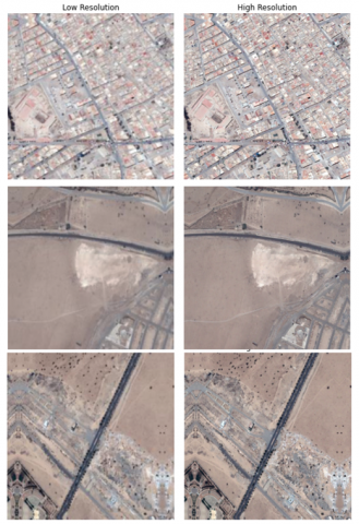
A high-resolution satellite image is an image with more details and conversely, an LR image is an image that lacks details. Moving from an LR image to an HR image, the details that are missing on the image which increases the spatial resolution of the image must be incorporated. Indeed, each time we increase the resolution, we see more details. This is highlighted in Figure 2 where we can see the visual effect of increasing the spatial resolution each time by a factor of 2.
Figure 2. Increase by a factor of 2 the spatial resolution of the image
The proposed solution allows the super-resolution of images. This scientific term refers to the scaling of images that can lead to a high-resolution image (HR) from a low-resolution version (LR) by applying a degradation function.
LR=D (HR, f). (2)
D is the degradation function and f is the scale factor. So, the Super-resolution is to learn the inverse function of Eq. (2) to reconstruct the image HR by applying the function of Eq. (3).
HR=SR (LR, f). (3)
The super-resolution thus allows gaining an image of better quality than the one that never existed or was lost. The details of the high-resolution image are filled in where the details are essentially unknown.
Figure 3. Classification of image super-resolution method
As you can see from the diagram in Figure 3, there are several approaches to super-resolution in the literature. Super-resolution image is mainly divided into SISR (Single Image Super-Resolution) and MISR (Multiple Image Super-Resolution) [26]. SISR provides a higher-quality image based on a single input image, while MISR provides a high-resolution image from a set of merged images of the same image [27]. SISR is more widely used than MISR due to its performance, processing simplicity, and researcher support as well as the flexibility of use [28]. In this paper, the focus is on learning-based approaches within SISR, to exploit the proven potential of deep learning in this direction.
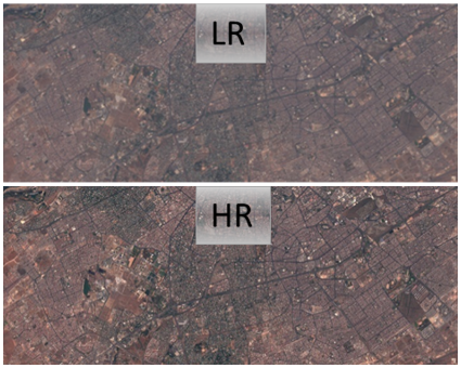
We recall that the founding principle of super-resolution by learning generally consists in reducing a target image to create an image of lower resolution, then scaling the latter by prediction. The predictive model must improve the low-resolution image to be as good (or better) than the target. To do this, the model (mathematical function) takes the low-resolution image that lacks detail and adds the details and features to it. Figure 4 shows the example of scaling a satellite image of the city of Rabat by prediction.
Figure 4. Super-resolution of a satellite image of the city of Rabat by deep learning
This approach will analyze and train from several images that have been reduced to create the lower spatial resolution input to reconstruct the details lost in the low-resolution image. It is, thus, a question of making it possible to synthesize a high-resolution image from its corresponding low-resolution image. This elicits incorporating imagery details from a higher resolution image into a deep neural network (DNN) and extracting the details to enhance geographically similar satellite imagery. However, applying directly the Super-Resolution methods to satellite images can help in obtaining spectral distortions [18], which requires a thorough study.
The study used benchmarks to decide the technical choice of the neural network adapted to the satellite imaging context. Indeed, there are many state-of-the-art solutions proposed in the rapidly growing field of super-resolution.
According to this benchmark [29] that is realized, the CNN is the most natural choice for the tasks of Super-resolution but the function of loss MSE (pixel loss), is adapted only to smooth images and does not give better results for images with finer textures as the case of the satellite images. Also, the use of the GAN [30] remains a choice by generating a clearer visual image, but this type of network requires more resource which is not adapted to the target study.
3.1 Adopted approach and method
The adopted approach capitalizes all the work done in SISR by deep learning and the strength of traditional methods. This approach benefits from all the progress made today in deep learning.
It is based on work done on satellite images; the design and architecture of some networks such as FSRCNN [31] and MFSRCNN [32] and this experience in satellite image processing. The latter cooperates with the best approaches to accelerate CNNs and increases the performance of network stability to get the best network allowing the Super-resolution of satellite images.
Figure 5. The global architecture of satellite image super-resolution network (FSRSI)
Based on the analysis, it is clear that the progress made in neural networks allows increasing the speed as the case of FSRCNN [31] which is fast, but it is limited in the construction of images with high-frequency details in the satellite images. Thus, the necessary improvements are made to achieve the objective.
Multi-scale fusion is efficient for the reconstruction of high-frequency details [18], so this model is based on this concept, inspired by the MFSRCNN [32] model, which is based on multi-scale fusion to keep the maximum of information. For example, low-resolution satellite images are sampled and down-sampled simultaneously to obtain sub-arrays that are connected in parallel which reduces the loss of information and guarantees a faithful reconstruction.
This model adopts an autonomous end-to-end learning pipeline [33], which allows for the Super-resolution of satellite images without pre-processing elsewhere in the network. additionally, its model uses small convolution kernels and more convolution layers.
This model encompasses 5 levels of resolution, which allows for a more reliable match between the low-frequency and high-frequency details of LR and HR images. Thus, the architecture consists of 5 sub-arrays of different scale factors (resolution) that are merged at the end to integrate all the features of the image. Also, a procedure is proceeded by residual learning which helps a lot to obtain efficient learning. The network manages the 13 bands of the sensor for a global reconstruction and simultaneous processing of the channels. A good balance of layers to gain non-linearity by increasing the abstraction is adapted to have more accuracy by reducing the dimensionality of the network.
Multiscale fusion allows an exchange between sub-networks to extract more detailed features within the satellite images by exploring the layers simultaneously. This multiscale processing allows controlling the difference in GSD on the different spectral bands of the image.
CNN capture features on normal images, but for satellite images, these features are different (since they are encapsulated as reflectivity), and even more important (depending on the spectral resolution), therefore; an experiment according to the study done by [10] on the contribution of the depth of the grating on the accuracy is conducted to find out a better balance on the depth of the grating. So, more filters are needed to obtain more information on the input image.
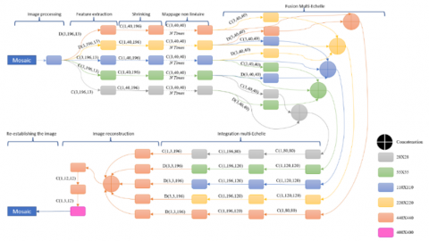
Moreover, from an architectural and technical point of view, the target FSRSI network is a fully convolutional neural network that uses the NIN principle [34] and proceeds in 6 main phases. The layout of these phases is shown in Figure 5 which shows the global architecture of this model and its design as a pipeline.
3.1.1 Image processing
From the satellite image, we proceed to the mosaic operation (cf. 3.2) to get an image of 110X110 Pixel. Thus, Figure 6 summarizes the performed mosaicking operation. This operation is well explained in the following section (cf. 3.3).
Figure 6. Process of the image processing stage
The spatial resolution for satellite images is an important characteristic. The Super-resolution must improve, so the resolution degradation process must be done appropriately unlike ordinary images. Consequently, we proceed to a resolution degradation in a learnable way integrated into this model. Then, we proceed to the oversampling (by deconvolution) and under-sampling (by convolution) of the LR image to get images of different resolutions (28X28, 55X55, 110X110, 220X220, 440X440) which constitute the entries of the 5 sub-networks. Thus, the enlargement of the images within the model is not done by interpolation but in a learnable way without losing the sense of detail as the interpolation is learned within the network according to the target image with learnable kernels as well (see 3.2.3).
This pre-processing phase consists of improving the contrast of the image before proceeding to the super-resolution process; this pre-processing consists of determining the areas of importance in the image for each spectral band by analyzing the histogram of each channel. Figure 7 shows the use of this method on the dataset elaborated as a spectral band histogram.
Figure 7. Histogram of band 4 of an input image
Thus, the interesting part of the image is around the peak and the contrast can be improved by cutting the regions around the contrast. This operation is called the equalization of the diagram and it shows a considerable contribution to the performance of the reconstruction of satellite images [18]. Figure 8 shows the result obtained after this operation.
Figure 8. Contrast enhancement of an input image
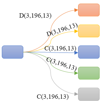
3.1.2 Feature extraction
The extraction of features is done directly on the original satellite image without interpolation by doing a convolution. Indeed, the number of convolution kernels is considerably increased in small size to have more features, and each kernel is sensitive to a specific spot contour, colors, edges, borders, ..., which allows extracting the maximum number of features. This phase is illustrated in Figure 9. As from the original input image, we proceed by convolution to resolve equal to or lower than the original, that is for resolutions of 110, 55, and 28 pixels. However, we proceed by deconvolution to reach a higher resolution than the original, that is for resolutions of 220 and 440. For the parameterization of the convolution (deconvolution), we adopt this annotation C (X, Y, Z) such that X is the size of the convolution filter, Y is the number of filters and Z is the number of input channels.
Figure 9. Feature extraction from the input image
3.1.3 Shrinking and non-linear transformation
Since the feature vector of the LR satellite image is of very high dimension, we will have an important computational complexity. So, we apply 1X1 convolutions to reduce the computational cost and for better restoration. This constraint forces to the addition of a shrinkage layer with several filters of 40 which is less than the starting number of 196, which considerably reduces the number of parameters.
We also use several layers of 3X3 and several mapping layers of 12 for a better compromise between the accuracy and complexity of mapping, which is illustrated in Figure 10, showing the reduction of the dimensionality.
Figure 10. Shrinking process and non-linear transformation
3.1.4 multi-scale fusion/integration
Figure 11 shows the process of fusing the feature maps which is done by concatenation and improves the accuracy of the super-resolution reconstruction [35], so we proceed to merge all the features from multiple scales. The fusion is done by upsampling or downsampling depending on the scale to adapt the adjacent networks. This is a key phase for the fusion of the features of several resolutions in order to better learn the details of the satellite image such that each sub-network of resolution proceeds by upsampling to the direct higher resolution and downsampling to the direct lower resolution and sends the clean result of its resolution. The set of results obtained is concatenated by resolution. This way of doing things has considerably improved the performance of both high and low-frequency detail reconstruction according to this experiment.
The deconvolution operation is done by transposed convolution. This layer aggregates the features with deconvolution filters for a scaling factor of 4. This layer efficiently trains the oversampling feature kernels. Figure 12 shows this integration process which allows to the integration of the set of features learned on each sub-network for each resolution. This integration proceeds by convolution and deconvolution in a reverse way to the feature extraction process which allows to the preparation of the network output.
Figure 11. Multi-scale fusion process
Figure 12. Multi-scale integration process
3.1.5 Image reconstruction
After the extraction of the features of the 5 sub-networks, we extend the dimension to the output and then we oversample the image to the size of 440X440 before restoring it to the size of 400X400 by exploiting the information of the padding carried out in mosaicking (cf. 3.2.2) to preserve the existing spatial hierarchy in the satellite image. Figure 13 shows this process, as we see, the concatenation of the features and the spreading at the output.
Figure 13. Image reconstruction process
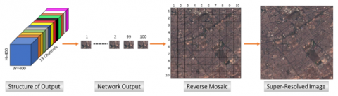
3.1.6 Restoration of the satellite image
At the end of the reconstruction of the index image (10, 10), that is to say, the last image of the same mosaic (last image of the batch), we must reconstruct the mosaic to have the same image at the output as the input image. This phase is detailed in Figure 14, which exploits the information of the mosaic that allows the reconstruction of the image transparently.
Figure 14. Image recovery process
The transfer of convolution filters takes good advantage of this multi-scale approach for fast convergence given the size of the data. The proposed model is based on several key factors for increasing the quality of satellite images. The separation between the convolution layers (which allow the extraction of features from the satellite images) and the deconvolution layers (which contain the scale factor information) combined with the principle of multi-scale aggregation are decisive for this model.
3.2 Application to satellite images
This section is devoted to the application of the adopted FSRSI model to the case of satellite images. This model takes into account the problems mentioned and the specificities of satellite images and ends with a fundamental approach of super-resolution adapted and a specific configuration and training.
To overcome the problems mentioned in the introduction, this model is first tested on compressed satellite images before opting for a generic solution that can be adapted to the case of satellite images, using the adopted model.
3.2.1 RGB satellite image compression approach
The first solution is inspired by the literature [36]. It consists in simply using RGB compression of satellite images. Otherwise, the idea is to compress multispectral images in RGB format, keeping only the RGB bands and eliminating the others. In the latter case, the loss of information carried by the eliminated bands can make the resulting super-resolved image inadequate for further processing in which this information is important.
On the other hand, compression can be carried out by image processing by analogy to the signal with Fourier transforms [37]. Indeed, several compression algorithms adapted to satellite images exist in the literature. They can be classified as lossless [38] or lossy [39] compression algorithms. This study proposes to opt for the lossless ones, given their performance, and to preserve the characteristics of the satellite images as much as possible. Compression would therefore be a simple solution that will allow proceeding later, by training similar to the case of ordinary RGB images.
3.2.2 FSRSI approach without compression and spectral dependence
To overcome all the problems related to the processing of multispectral and hyperspectral images without loss of information due to compression, this study proposes a new generic approach to adapt to the different types of these images including satellite images. This solution consists in adapting the data as well as improving the scalability of the model (its scaling) for a better reconstruction and to overcome the normalization problem.
Indeed, to overcome the processing complexity problem due to the volumetry of the images because of their size and the multiplicity of bands, this study proposes to exploit the mosaic functionality to split them into scenes relative to the tiles that constitute them while preserving and taking into account the spatial dependencies between them. An additional phase has been added to the network to have a training dataset consisting of a sequence of images (scenes) in a grid that takes into account their spatial positions.
This feature, we propose, is a data propagation tool on the CNN that allows to management and query of the data and metadata of the satellite images. It is a powerful model in the form of a catalog that provides the source of each pixel on the image, and a set of rules to treat the tiles in the same way as treat the original image. We also indexed this dataset for better management and to optimize the model. This method allows to the management of several resolutions to take care of all the spectral bands of the Sentinel-2 image. Thus, the mosaic manages each spectral band in a transparent way and without loss of any pixel since we do not make any modifications to the original image. But it is a virtual layer that is added and manages the processing, so we pass the image on the network through a mosaic that decomposes it into tiles, and at the output, we will have a super-resolved satellite image reconstructed by the same mosaic.
The displacement within the mosaic is done in the same way as a filter within a CNN with 10 pixels. To stay in the logic of a global image, if the displacement is not done with a stride, it is like dividing the image into individual parts. In this case, we will call it padding in the same way as deep learning; except that for us. Padding is not done to add space around the input image but to preserve the spatial dimension and capture the information at the edges of the resulting images of the mosaic in a homogeneous way.
The act of not using padding does not allow inspecting the edges of the input image with filters when extracting features by convolution. The experiment has shown that a padding of 5% to 15% of the size of the resulting image of the mosaic should be used, to preserve the information on the edge and not to degrade the inference speed of the model.
Figure 15. Impossible positions without considering the padding
Figure 16. Inspection of image edges using mosaic padding
Thus, the positions of the filter mentioned in red (Figure 15) can only be taken on the input image after considering the padding which allows capturing the information at the edges of the image, which gives the possibility to treat the whole satellite image as a single block. So, the padding avoids losing the spatial dimension which is crucial for georeferenced satellite images.
The use of padding allows capturing of the positions on the edges of the image (Figure 16) and to detection of the features on the borders of the image in the same way as in the center of the image.
There is no type of filling specified in deep learning that can be used because they are not adapted to this case but this study tries to adopt a specific filling according to the position of the image on the mosaic; thus, Figure 17 shows the padding constitution according to the spatial position of the satellite image.
Figure 17. Constitution of the images with a stride of 10 according to the position within the mosaic
The mosaic allows choosing of a good spatial hierarchy to decompose the satellite image. Indeed, thanks to the distribution of the satellite image in mosaic format, the proposed model creates a spatial hierarchy in the same way that the network does for the creation of feature maps. Experience has shown that this way of doing things improves the network performance considerably while preserving the distribution of the satellite images on the edges.
Satellite images are a very special case of images that comprise a variety of spectral bands belonging to different interval waves, and if not normalized they become ill-suited to CNN processing generating an internal covariance mismatch that relates to the changing distributions of the input data for each hidden layer, which increases the computation time and may lead to non-convergence, or the impossibility of learning the Super-Resolution function as a whole [32]. Indeed, to overcome this problem, which is directly related to the normalization problem, we propose to use batch normalization [40] which reduces the distribution of data to an interval [0-1], and not resort to a normalization of the values of the bands through the calculation of their average from the beginning and at the start of the training, but to proceed by a separate training of the bands giving rise to as many feature maps as there are bands and to capitalize at the end, on the set of maps to reconstruct the output image. This study also proposes to take into account the dependency (correlation) between the bands due to the overlaps that may exist between them within the images. To do this, an adaptation of the algorithms of the adopted model was necessary to develop this solution.
Indeed, the exploitation of the spectral dependence allows to solve the spectral variance problem [41] and to eliminate the redundant information within the satellite image in a learnable and efficient way that reduces redundant parameters and accelerates the network.
3.2.3 FSRSI approach with spectral dependence
In addition to the approach used in the previous section, this study also proposes to take into account the dependence (correlation) between the bands due to the overlaps that may exist between them within the images, to see the effect of taking into account this spectral dependence on the performance and processing time. To do this, a spectral correlation module was added to the network to develop this solution. This module works in collaboration with the feature fusion module as the spectral correlation is only a fusion of spectral features on several levels that are the sub-networks of different resolutions. this module of exploitation of spectral correlation uses 3D convolutions that are best suited to capture more features.
Indeed, the exploitation of the spectral dependence allows to solve the problem of spectral variance [41] and to eliminate the redundant information in the satellite image in an efficient and learning way that reduces the redundant parameters and accelerates the network.
3.3 Parameterization and optimization
After the implementation of the model, it was necessary to proceed to the configuration of its learning to improve its performance. This parameterization consists of the redefinition of the hyperparameters or the change of the number of feature extraction layers, but also the consideration of certain techniques for its optimization. After several attempts to train the model with different configurations for the three previously proposed solutions, we ended up adopting the optimal configurations needed to give the best performance. Regarding the Adam optimizer [42] used for the optimization of the computation time and convergence rate (number of iterations before convergence), we point out that it starts with an initial learning rate (the speed at which the weights are adjusted) of 0.0001 for the convolution layers while it is 10-4 for the Deconvolution layers to minimize the losses and adjusts this rate when the loss does not decrease after 5 epochs of training. The training rate is reduced by a factor of 2 and terminated when the learning rate is less than 0.00002.
The depth of the considered convolution layers varies between 196 and 64 depending on the 1x1 and 3x3 convolutions. The step size is 1 and the size of the convolution kernels is 3x3 for better reconstruction quality, and zero padding is used in the reconstruction step to keep the output image size and avoid truncation errors [43].
The convolution for the no linear mapping layer is a 1×1 convolution AS suggested also in Network in Network (NIN) [34]. In NIN, 1×1 convolution is suggested to introduce more nonlinearity to improve accuracy. It is also suggested in Google Net [36] to reduce the number of connections. The 1×1 convolution is used as a dimension-reduction module to reduce the computation. By reducing the computational bottleneck, the depth and width can be increased. The 1×1 convolution can help to reduce the model size, which can also somehow help to reduce the overfitting problem.
The proposed model uses a MaxPooling of 2x2 and a batch size of 100 to process images of the same scene within the same learning epoch. Moreover, the initialization of the weights has been done by the Xavier method and the initialization of the convolution layers has been done by the normal distribution.
Regarding the activation function, the model use PRelu, which is claimed to be better than Relu, it is a kind of Relu leakage where the network decides the value of the slope instead of a predefined slope of 0.01. It is defined by y=ax when x<0 and y=x when x>0 where a is a parameter to be determined by the network.
The cost function is just the standard mean square error (MSE) (Eq. (4)), which WELL fits in the Super-resolution context [44].
$\min _\beta \frac{1}{n} \sum_{i=1}^n\left(\left\|F\left(Y_s^i, \beta\right)-X^i\right\|\right)_2^2$ (4)
Based on the accumulated experience, one should have a larger number of filters to get slightly better results. But in fact, the number of layers is limited, it is not enough to prove it. They should also increase the layers. If there are more layers, larger filters can be replaced by several smaller filters. This is what we have done in the network to take advantage of NIN's capabilities.
However; experience has shown that the efficiency of CNNs in Super-resolution is not directly related to depth as the case for classification which requires a good compromise between performance and computation time. For instance, we can increase the performance by adding more filters but for satellite image time, IT is of the essence (drastic increase in time). This experience has shown that we increase complexity for benefiting from little performance. This network works in 5 parallel networks which benefits the optimization of the architecture.
A sentinel image is a product in the form of tiles of 100*100km with a spatial resolution of 10 to 60m and 13 spectral bands. The size of an image is, therefore (104X104X13) pixels. So, a single layer of convolution trained on this image will take 2.3x10¹² multiplications for a filter of 196.
NM/P= Kernel width x Kernel height x Number of channels x Number of kernels x Number of vertical slides x Number of horizontal slides=3X3X13X196X104X104=2.3x10¹².
In this case, we can use spatially separated convolutions [44] which require only 20% of the necessary multiplications, however, this technique is not adapted to this satellite context where the spatial reference for the pixel is important during training.
On the other hand, FSRSI uses convolutional layers separated in depth [45]. We will have 10E4*10E4 individual convolution; in total 9x10¹⁰.
Considering the mosaic gives 112X112 individual convolution which is in total 110X110X13X3X1=145 for the convolution operation in depth and 110X110X196X13=3X10⁷ for the point convolution operation which gives in total 322X105.
This proves the use of separate depth convolutions in the neural network.
So, Table 1 presents the implementation details and the parameterization (including hyper-parameters) of the model.
This parameterization allows a better efficient convergence with a minimal error rate and avoids the degradation problem. The choice of this parameterization was made following several experiments and analyses of the influence of each parameter and its adaptability to the model to have this optimal configuration for the super-resolution of satellite images which offers a better compromise between the quality of the super-resolved image and the complexity of the model.
These improvements allow the proposed network to benefit from better performance with an improvement in computation time and an adaptation for the processing of satellite images. Thus, a better testing and training strategy is adopted for better speed and performance.
Table 1. Parametrization of the model
|
Parameters |
Value |
|
Layers |
12 |
|
Filters |
196 |
|
Min filters |
64 |
|
Training images |
3000 |
|
24000 |
|
|
Dropout rate |
0.8 |
|
Batch image size |
100 |
|
Batch num |
240 |
|
Filters decay gamma |
1.5 |
|
Self-ensemble |
8 |
|
Clipping norm |
5 |
|
Activation Function |
Prelu |
|
Loss function |
MSE |
|
Metrics |
PSNR/SSIM |
|
Convolutions |
1X1/3X3 |
|
Optimizer |
Adam |
|
Initial learning rate |
0,0001 |
|
learning rate for Deconvolution layers |
0,00001 |
|
Reduction factor (learning rate) |
2 |
|
Limit learning rate |
0,00002 |
|
Step size |
1 |
|
Convolution kernels |
3x3 |
|
No linear mapping convolution |
1X1 |
|
Pooling |
MaxPooling 2x2 |
|
Initialization weights |
Xavier |
|
Initialization of the convolution |
normal distribution |
|
Convolution type |
separate depth convolutions |
3.4 Data-augmentation
Since network performance increases with the amount of data, this model uses the increase in data to expand the dataset with new examples to increase the diversity in the training satellite images. We reinforce the instance-based data augmentation strategy through the work done by the study [46] to add the channel aspect by merging channels following this model which applies a spectral and spatial fusion method without forgetting the effect of spectral dependence. This approach consists of adding artificial bands with additional information. It is effective in increasing the PSNR, according to an experiment we have performed.
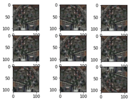
So that the transformations below are applied by realistic transformations to the case of satellite images, this choice was made carefully after several experiments by measuring the contribution of the transformations to the performances and by realizing a better compromise between the spatial invariance introduced by the data augmentation and the spatial dependence imposed by the georeferencing of the satellite images. For the increase of the horizontal and vertical offset, we use a minimal transformation of 10 pixels with a filling from the pixels of the global satellite image. Figure 18 shows an example of visualization after the application of this transformation.
In the case of satellite images, the shift has a direction that determines the shooting angle which should not influence the model; therefore, this study uses the vertical and horizontal shift to break the strong coupling with the shooting angle. Figure 19 shows an example of visualization after the application of this transformation.
Figure 18. Data-augmentation of the horizontal and vertical shift (width_shift_range= [-10,10])
Figure 19. Data-augmentation of the flip (horizontal_flip=True; vertical_flip=True)
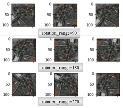
For the angle of rotation and the same reasons mentioned before, the 90, 180, and 270 angles are adopted. Figure 20 shows an example of visualization after the application of this transformation.
Figure 20. Data-augmentation of the rotation (rotation_range=90;180;270)
Figure 21. Data-augmentation of brightness (brightness_range= [0.2,1.2])
The random increase in brightness is also interesting to break the coupling with the atmospheric conditions and the time of day when the image was taken, so the proposed method applies both lighting and shading. Figure 21 shows an example of visualization after the application of this transformation.
Table 2 summarizes the parameters adopted for the data augmentation.
Table 2. Parametrization of the data-augmentation
|
Parameters |
Value |
|
Width shift range |
[-10,10] |
|
horizontal flip |
True |
|
vertical flip |
True |
|
rotation range |
90;180;270 |
|
brightness range |
[0.2,1.2] |
3.5 Degradation process
The degradation method is important in the Super-resolution process since it determines the way the images are reconstructed, and mastering it allows for the improvement of the deep learning model. Most of the models use high-resolution images and apply a traditional input such as interpolation to reach the desired size according to the scale factor. Figure 22 shows visualizations to see the effect of each type of interpolation on the structure and quality of the reconstructed image.
Figure 22. Effect of interpolation on an input image
Figure 23. Visualization of the filters and their frequency responses
Thus, we deduce that the use of interpolation deteriorates the fidelity of the satellite image and alters the information within this image.
In addition, other methods use filters through convolution kernels, which led to testing some filters on input images to see their effects on the degradation method of the satellite images. Thus, the construction of a Gaussian kernel of the size of the input image with a deviation of 1 and a uniform kernel with a deviation of 5, allows to better understand this concept.
Figure 23 visualizes the filters and the Fourier transform modules for their frequency responses.
So, this study considers a degradation function (Eq. (5)).
LR=D(C(HR), α) (5)
D is the degradation function; C is the convolution operator and alpha is the degradation parameter. For the degradation, we consider a Gaussian blur and a disturbance in the form of additive Gaussian noise of variance α= σ2.
Figure 24 gives a visualization of the degraded image considering the Gaussian filter. From this visualization, we deduce that the proposed method uses only the Gaussian fuzzy for the degradation.
Figure 24. Visualization of the blur and the Gaussian noise
This approach consists of using a learnable degradation method within the model which avoids all the problems mentioned before and which improves considerably the performances of the model with a real degradation adapted to the case of satellite images. Thus, the model uses a learnable interpolation that keeps the spatial and frequency structure of the details by adapted learning within the network according to the output image (according to the scale factor) with learnable convolution kernels (filters) which gives a better perceptual quality [47] and a flexible pipeline.
4.1 Basic super-resolution approach adopted
Indeed, the super-resolution of satellite images consists of reducing the GSD of the image to increase its resolution. To achieve this objective, the fundamental approach that we adopt is to transform the super-resolution objective which is a poorly posed optimization problem into a well-posed inverse problem. The idea is to degrade HR images (to increase the GSD) and optimize the super-resolution algorithm so that it learns and generates HRS images (oversampled HR) and thus reconstructs the original images from the degraded images.
Note that we must calculate performance metrics such as the maximum signal-to-noise ratio (PSNR) [48] and SSIM [48] to measure the difference between the original image and the reconstructed image, and thus evaluate the relevance of the model learning.
4.2 Performance measurement metrics
PSNR (Peak Signal to Noise Ratio) is a measure of the reconstruction quality of a digital image. It measures the reconstruction performance of the super-resolved image compared to the original image.
The PSNR is inversely proportional to the logarithm of the mean square error (MSE) (Eq. (6)) [48] between the ground truth image and the super-resolved image.
PSNR (Peak Signal to Noise Ratio) (Eq. (7)) measures the reconstruction quality of the super-resolved image compared to the original image.
$\operatorname{MSE}(x, y)=\frac{1}{N M} \sum_{i=1}^N \sum_{j=1}^M\left(x_{i j}-y_{i j}\right)^2$ (6)
${PSNR}(x, y)=10 \cdot \log _{10}\left(\frac{L^2}{M S E(x, y)}\right)$ (7)
MXN is the size of the image and L is the maximum possible value of the pixel (for RGB bands, it is 255).
However, this measure does not take into account the visual reconstruction which can influence the reconstruction at high-frequency details hence the need for SSIM.
The structural similarity or SSIM [48] (Eq. (8)) measures the visual quality of the super-resolved image as a function of the structural similarity to the original image by assuming that the human eye is sensitive to changes in image structure. Thus, we apply the formula of Eq. (8) to the luminance on 2 windows x and y of size 8x8. the equation is composed of the scalar products of the terms A (Eq. (9)), B (Eq. 10), and C (Eq. (11)).
${SSIM}(x, y)=A(x, y) . B(x, y) . C(x, y)$ (8)
$A(x, y)=\frac{2 \mu_x \mu_y+E_1}{\mu_x^2+\mu_y^2+E_1}$ (9)
$B(x, y)=\frac{2 \sigma_x \sigma_y+E_2}{\sigma_x^2+\sigma_y^2+E_2}$ (10)
$C(x, y)=\frac{\sigma_{x y}+E_3}{\sigma_x \sigma_y+E_3}$ (11)
With x the ground truth image; y the super-resolved image; $\mu_x$ the mean of x; $\mu_y$ the mean of y; $\sigma_x^2$ the variance of x; $\sigma_y^2$ the variance of y; $\sigma_{xy}$ the covariance of x and y;
$E_1=\left(K_1 L\right)^2 ; E_2=\left(K_2 L\right)^2 ; E_3=\frac{E_2}{2}$; L the dynamic of the pixel values, which is 255 for the 8-bit coding; K1=0,01; K2=0,03.
E1, E2 and E3 are intended to stabilize the ratio when the denominator is very low.
However, we consider only a subset of these windows to reduce the complexity of the calculation.
Thus, we need to establish a balance between the performance using these performance metrics and the perceptual quality of the satellite images which we apply in the approach adopted.
4.3 Datasets
To demonstrate the interest in the approach adopted, we use free high-resolution raw satellite images. These images are provided by the Sentinel-2 satellite of the European Space Agency as part of the Copernicus program for environmental monitoring, the latter is composed of a constellation of 2 satellites on the same orbit, they are multi-spectral optical images with 13 spectral bands and a revisit capacity of 5 days [49]. Table 3 shows the characteristics of Sentinel's MSI sensor bands.
Table 3. Spectral bands of the MSI sensor of the Sentinel-2
|
Bands |
Wavelength (nm) |
Spatial resolution (m) |
|
Tape 1 - Coastal Spray |
442.7 |
60 |
|
Band 2 - Blue |
492.4 |
10 |
|
Band 3 - Green |
559.8 |
10 |
|
Band 4 - Red |
664.6 |
10 |
|
Band 5 - Red edge vegetation |
704.1 |
20 |
|
Band 6 - Red edge vegetation |
740.5 |
20 |
|
Band 7 - Red Edge Vegetation |
782.8 |
20 |
|
Band 8 - PIR |
832.8 |
10 |
|
Band 8A - PIR "narrow |
864.7 |
20 |
|
Band 9 - Water vapor |
945.1 |
60 |
|
Band 10 - SWIR - Cirrus |
1373.5 |
60 |
|
Band 11 - SWIR |
1613.7 |
20 |
|
Band 12 - SWIR |
2202.4 |
20 |
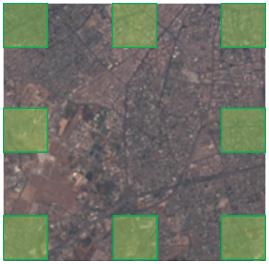
The whole dataset includes 240 scenes (30 regions -shown in Figure 25- taken twice a day from 50 km2 over the 4 seasons of the year) - without Data Augmentation-; These images of Morocco are taken to cover all the regions to cover the mountainous, aquatic desert and forest areas as well as areas with urban concentration and others with more details, which are taken throughout the year to cover all seasons. We tried to provide a variety of images to benefit from the model performance, taking advantage of the spatial invariance. Table 4 presents the characteristics of this dataset.
Table 4. Description of the dataset used for training and testing
|
Dataset |
Sentinel-2 |
|
Original Size |
30*4*2=240 |
|
After Mosaic Size |
24000 |
|
Spatial Resolution |
10m, 20m, 60m |
|
Avg. Pixels |
10E4*10E4 |
|
Avg. Pixels (After Mosaic) |
100*100 |
|
Format |
JPEG 2000 |
|
Encoding |
16 bits |
|
Spectral resolution |
13 bands |
|
Wavelength |
442.7-2202.4nm |
Morocco is a typical example of the application of Super-resolution, this country includes both the Mediterranean, a continental, and a desert climate and an important mountain range and a forest cover. This climatic diversity gives a great possibility of generalization of the proposed model on satellite images on the world level.
This dataset was divided into 192 scenes for training and 48 scenes for testing.
Figure 25. Morocco coverage of the training set
The images chosen are very appropriate for training given the criteria set for this study. In addition to the diversity within the data, this approach also involves taking clear images (cloud cover is less than 20%).
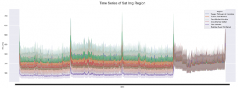
The processing of images taken in the same location at each season will be considered as a time series at an interval of 3 months. The approach adopted is to define the same conditions for each image taken at the same interval to follow the trends of the seasonal component in the satellite image, so we are facing a univariate time series. Thus, Figure 26 represents the time series of satellite images taken throughout the year over the 4 seasons.
Figure 26. Time series of the number of images taken throughout the year by the administrative region of Morocco
Figure 26 shows that there is a balance between regions for the number of images taken for the first 3 seasons including spring, summer, and autumn, however, for the winter this number varies depending on atmospheric conditions which sometimes makes the images unusable.
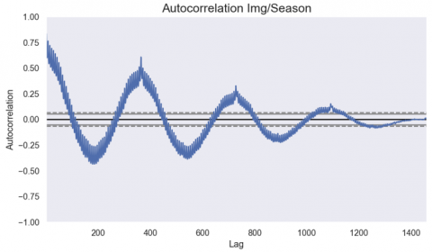
In addition, we determine the autocorrelation within the images taken for each region to determine the repeatable images for each season. Thus, Figure 27 determines this process.
Thus, thanks to this process, the realized approach eliminates the seasonal component and gives the model a great generalization capacity.
For the compression solution, the model was adopted to exploit the quick looks of the images, that is a spatial and spectral subset of the original images. These images are produced in true color at a GSD of 320m, which gives images 313X313 of RGB pixels. For each area, we take 100 images to cover different periods and different climatic conditions. The constructed dataset, therefore, contains 2400 images for training and 600 for testing to benefit from the Bigdata performance of the model.
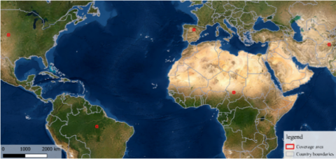
To demonstrate the generality of the model and the reproducibility of the results, a validation on satellite images from all over the world with different characteristics is necessary; thus, the model has been tested on 5 images representative of the 4 continents (Figure 28) which constitute the validation set of the model in the same way as the images taken from Morocco (20 scenes distributed over the 4 seasons).
Figure 27. Autocorrelation of satellite images by season in the Tanger-Tetouan-Al Hoceima region
Figure 28. Global coverage of the validation set
4.4 Training details
The model is realized with the Tensorflow framework [50] with Keras [51] in the backend, using a GPU (in the form of 2 graphics cards Nvidia GeForce and Nvidia Quadro). The use of tensorboard [52] allowed to follow the training process of the model and visualize its performances.
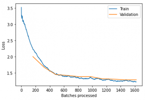
Figure 29. Visualization of the loss of the model over the epochs
From Figure 29 we can see that the metric is not too sensitive to the variation of the weights over the epochs and that it drops efficiently, such that it drops rapidly at the beginning but slowly at the end (for the test in particular), which proves the performance of the model. The experiment shows that the model can be further improved, but experience shows that increasing the number of epochs will result in a longer processing time with a very marginal improvement.
Moreover, the visualization of the evolution of the training of the model allows to better understand it through different aspects (weight, bias, gradient).
Figure 30. Visualization of the progression of aspects of the learning model
The visualizations in Figure 30 allow seeing the set of aspects influencing the learning of the model. Thus, we can see the distribution of weights on the histogram to see the usefulness and contribution of each layer in learning and the efficiency of the model architecture. As a result, the model, we can see that it has well adapted to the weights during the learning process by significantly adjusting the biases, which has allowed it to have better performances.
This section discusses the results obtained after the experimentation of the model, and the results of the experimentation while drawing up and discussing the results obtained.
This approach goes beyond the traditional methods (which use several images of a scene) and interpolation methods and approaches the results obtained on non-satellite images.
This network keeps a minimal blurring effect on the satellite image but the image is enlarged without noise with better features for edges and clearer details in addition to a better background, so this network displays a better PSNR and better image quality with a more realistic restoration.
5.1 Experimental results of RGB satellite image compression approach
Table 5. The overall result of the model for the dataset-based compression approach
|
Datasets |
PSNR |
SSIM |
|
600 images (20 images par zone) |
23,62 |
0,6590 |
|
1800 (60 images per zone) |
27,05 |
0,7726 |
|
3000 (100 images per zone) |
29,91 |
0,7956 |
Table 5 presents the training and test results of the model applied to the dataset used (without consideration of the data augmentation) for compressed satellite images.
Figure 31 illustrates by an example of an image, the result obtained during the test of the model. It represents an authentic image on the left and the corresponding super-resolved image on the right.
Figure 31. The visual result of the compression solution
The experimentation carried out shows that the perception (PSNR) and visual (SSIM) qualities ARE improved significantly, especially with a dataset of 100 images per area (beyond this value, we notice a minimal improvement of the model performances with an increase of the model complexity); the super-resolution of these satellite images has made it possible to make the image clearer by recovering interesting details for the visualization of relief and planimetry. However, this approach does not allow more zoom on the resulting image since the recovered details are less important. Since the work was done on compressed images with a loss of information.
Thus, this solution is not adapted to the case of multispectral satellite images and does not allow more zoom, and ignores the important information relating to other spectral bands, which makes the resulting image unusable except for the visualization in true color.
5.2 Summary of the experimentation of the FSRSI approach without compression and spectral dependence
To train the model for multispectral satellite images, the Sentinel dataset based on 16-bit coded (unsigned) JPEG2000 mosaics were used. In addition, it was also a question of performing a degradation (see degradation) of the resolution of the images before training and testing, and validation in the same way as for the compression case.
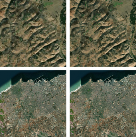
The results of applying the solution to the Sentinel dataset without compression are presented. We note that in this case, we experimented with the solution without taking into account the dependencies between the bands to confirm or deny their impact on the result. Figure 32 shows a sample of the visual results of this solution on the elaborated dataset. From this figure, we notice a clear improvement in the visual quality of the satellite images after Super-Resolution.
Figure 32. The visual result of the solution without compression and dependence
The obtained result demonstrated the performance of the model for the super-resolution of multispectral satellite images; indeed, the training and testing of the model resulted in a global average PSNR of 30.42db. (since the enhancement is not unformed on the image) and an SSIM of 0.89 which is relevant for the case of the satellite images for a factor of 4. Table 6 presents the performance of the approach without spectral dependence.
Table 6. Results obtained after training and testing the model
|
Metric |
Performance |
|
PSNR |
30.42db |
|
SSIM |
0.89 |
Figure 33. Zoom on a boat in the port of Casablanca
The analysis made on the images obtained has allowed deducing that the noise is higher in specific areas AND is less in other areas. In addition, Figure 33 shows a zoom (on a boat) of the test image before and after the model test. The visual and perceptual quality has been improved by the proposed model. We can see that the model has improved the visual and perceptual quality. The improvement of the perceptual quality concerned the areas or objects of heterogeneous structures (boats, constructions...). While for those of homogeneous structures (sea area for example), we note a clear improvement but with a little noise that does not alter the reality of satellite images.
5.3 Summary of the experimentation of the FSRSI approach with spectral dependence
To train the model for multispectral satellite images, we used the Sentinel dataset. The images cover non-overlapping areas of Morocco. Thus, we present this time, the results of applying this solution to the Sentinel dataset (13 bands multispectral images) without compression, but taking into account the dependencies between bands.
The overlap between the intervals of the spectral bands constituting a satellite image gives rise to a dependence between the bands by an inter-spectral correlation, which led this study to push the research and exploit this correlation in the training of the model.
A comparison of the results was also made of this experiment with those of the application without compression and dependency after reducing the bands of the trained and tested images to only 3 bands. The objective is to confirm or deny the impact of taking into account the dependencies between the bands.
The training and testing of the model have allowed for obtaining even better performances and very satisfactory results with a global average PSNR of 32.18db and an SSIM of 0.9186.
Table 7. Results obtained after training and testing the model with spectral dependence
|
Metric |
Performance |
|
PSNR |
30.42db |
|
SSIM |
0.89 |
Table 7 shows that the performance is improved by taking into account the spectral dependence, (+ 2.24 dB) with a net improvement of the convergence speed (the time is improved by a factor of 1.7).
We notice a clear improvement in the visual and perceptual quality by using a multispectral Super-Resolution with spectral dependence. Taking into account the spectral dependencies between the bands has improved the performance of the proposed model and the quality of the reconstructed satellite images. Moreover, this solution showed a great generalization capacity by improving test images completely different from the training one. Nevertheless, we can notice that as was the case for the second experimentation (section 5.2), the improvement concerned mainly the areas or objects of heterogeneous structures (non-water). While for those of homogeneous structures (sea area), minimal noise was found that only influences the human visual perception keeping the reliability of the information on the concerned areas. However, it is possible to use a frequency filtering method to reduce the noise to increase the human visual quality, but this method alters the spectral information within the satellite images. Nevertheless, the method AIMS to improve, all the same, the areas of heterogeneous structures mainly targeted by the super-resolution and to improve the quality of restoration of homogeneous areas, as well as the overall visual quality in a satisfactory way.
Thus, we compare the model to the state-of-the-art methods proposed for the super-resolution of satellite images for scale factor 4. This comparison was first made with the standard reference method which is the bicubic interpolation, before being made with the other methods namely: Auto-en [13], SARNet8 [53], NLB-HMS3D [18], SSPSR [54], MCNet [55], 3DFCNN [56], GDRRN [57], VDSR [11], EDSR [12], SRCNN [58], SRDCN [59] and RCAN [60]. This comparison is not exhaustive but includes networks with public implementations and architectures that support the input dataset so that the comparison is fair.
Table 8. Quantitative comparison of super-resolution models for scale factor 4
|
Method |
PSNR |
SSIM |
|
Bicubic |
29,471 |
0,936 |
|
Auto-en |
32,415 |
0,990 |
|
SARNet8 |
33,578 |
0,990 |
|
FSRSI |
33,616 |
0,988 |
|
NLB-HMS3D |
33,331 |
0,983 |
|
SSPSR |
33,201 |
0,979 |
|
MCNet |
33,045 |
0,974 |
|
3DFCNN |
32,486 |
0,958 |
|
GDRRN |
32,950 |
0,971 |
|
VDSR |
32,739 |
0,965 |
|
EDSR |
33,178 |
0,978 |
|
SRCNN |
32,414 |
0,956 |
|
RCAN |
32,632 |
0,962 |
From Table 8, we can see that the model has the best PSNR compared to the other state-of-the-art models, which proves the capability of the model in reconstruction, however for the SSIM, we find that other models are better with a very reduced factor (these models only focus on the spatial information exploration but ignore the spectral component, so they will have less performance for the other metrics) Thus, the model shows a global average PSNR of 0.038 dB compared to the following network, otherwise, for the other metrics, the model is even better.
The model shows better performance in other metrics that are essential for measuring the performance of models for super-resolution of multispectral satellite images. Thus, Table 9 presents the performance of the FSRSI model in spectral angle mapper (SAM) [61]; root means square error (RMSE) [62]; Relative dimensionless global error synthesis (ERGAS) [63], and cross-correlation (CC) [64].
Table 9. Quantitative performance in other metrics
|
Metric |
Performance |
|
SAM |
2,8431 |
|
RMSE |
0,0269 |
|
ERGAS |
5,7324 |
|
CC |
0,9216 |
5.4 Computational time
To highlight the speed of the model, a comparison to a standard CNN (SRCNN [58]) for Super-Resolution was done first before comparing it to a faster version considered in the literature (FSRCNN [31]). To do this, a time complexity analysis of the algorithms [65] was done.
Thus, the computational complexity for SRCNN is of the order of Eq. (12).
Comp= O{(f12n1+n1f22n2+n2f32) SHR} (12)
This complexity is proportional to the size of the HR image. The larger the HR image, the higher the complexity. If we take a Sentinel-2 satellite image we have an image with 13 spectral bands and a size of 10000X10000 so if we consider a standard SRCNN we have Eq. (13).
Comp=O{(81*64+64*1*32+32*25)13*208}=O{2013} (13)
However, for FSRCNN, the complexity is of the order of Eq. (14).
$C o m p=O\{(25 d+s d+9 m s 2+d s+81 d) S L R\}=O\{(9 m s 2+2 s d+106 d) S L R\}$ (14)
This complexity is proportional to the size of the LR image, which is much smaller than the SRCNN. So the satellite image (if we consider a scale factor of 2) is of the order of Eq. (15).
${ Comp }=O\{(9 * 4 * 144+2 * 12 * 56+106 * 56) 13 * 10 E 4\}=O\{15 * 10 E 8\}$ (15)
For the computation time, SRCNN needs a speed of 19m/s; while FRSCNN needs only almost 1m/s.
Moreover, the model has a complexity of the order of O{10E5}, which requires a computation time of 6*10-5m/s.
However, the space complexity also counts for this case but it is an outdated problem nowadays given the available storage space allocation.
5.5 Discussion
The adopted approach takes into consideration all the specifications of the satellite images. The model is effective for the super-resolution of multispectral satellite images without data loss with a reliable transformation. Thus, this study has allowed to set up a new global approach adapted for multispectral images, giving an efficient and optimal model with better performances by approaching the cases of ordinary images but keeping the reality of spatial images.
This method capitalizes on all the advantages realized in all types of networks but adapted to the adopted design. Indeed, FSRSI has a relatively shallow network, with an optimal architecture. It is even faster with a better quality of the reconstructed image. Indeed, the examination of the results obtained confirms the choice of this design which presents remarkable results in terms of signal similarity and visual quality for the super-resolution of multispectral images. In addition, the architectural features and technical parameters allow for better performance in terms of the quality of the result, but without increasing the computation time and complexity too much. We also add that the number of parameters for FSRSI is extremely reduced, which allows for a decrease in the computations required for the super-resolution processing of satellite images.
Thus, the proposed network can reconstruct fine textures and realistic details that are essential for a better perceptual quality of satellite images that have the particularity of having fine details and are important for interpretation.
The FSRCNN model can be considered as a network that provides, a more powerful expression of features and learning of correlations of features of intermediate layers. This CNN model encompasses all the capabilities allowed nowadays to be an unavoidable choice for the Super-Resolution of multispectral images. Composed of 6 steps and a set of modules, thanks to its simplicity, it is faster than other SISR algorithms for satellite images and offers superior performance in most cases in terms of PSNR [18].
In the FSRSI model, the mapping is learned directly without going through interpolation but directly from the LR image, with reduced input dimensionality. Thus, FSRSI makes better use of 1×1 convolution which is used between two convolutions to reduce the number of connections (parameters). By reducing the parameters, we only need fewer multiplication and addition operations, and ultimately speed up the network. This is why FSRSI is faster than other models proposed in the literature.
In addition, FSRSI also uses multiple 3X3 convolutions which reduces complexity by reducing the filter size. Thus, with fewer parameters to learn, it is better to have faster convergence and reduced overlearning problems. In addition, the filter size is smaller and the number of filters is lower, with only 12464 parameters and an even higher PSNR. This improvement is because there are fewer parameters to train, which facilitates convergence. Thus, FSRSI generates the super-resolved image from a deconvolution layer, which reduces the computational load, improves the speed, and results in a higher-quality image.
The results obtained allow to conclude that the empirical experimentation performed has confirmed the model adaptation to super-resolution of multispectral satellite images. However, FSRSI is a global model, generic and better adapted to all types of images (RGB, monochrome or multispectral). Its results remain satisfactory.
The use of the compression approach allows to prove first of all the use of the model for the treatment of RGB images, but especially that this approach is not at all adapted to the treatment of multispectral images, where the spatial information is encapsulated in spectral bands other than the RGB channels.
Moreover, the spectral dependence between the bands allows further improvement to the visual and perceptual quality as well as the reconstruction accuracy with an even better inference speed and a great generalization capacity.
Multiscale fusion has improved the efficiency of the model, which is a key to the success of the method in terms of efficient reconstruction of high and low-frequency details. This technique allows keeping a maximum of information within the image, thus more details, and a better resolution. The information fusion guarantees a faithful reconstruction taking into account the real character of the satellite images and the spatial coherence, as well as a good consideration of the difference in GSD within the Sentinel-2 dataset images. This technique allows a multi-level exchange of the extracted features within the intermediate layers.
The proposed network shows good image detail recovery and efficient edge reconstruction, in addition to high generalization capability by demonstrating its global reusability. However, MSE favors a high PSNR, but the model also showed satisfactory performance in other metrics mainly SSIM, but also in SAM, RMSE, ERGAS, and CC.
The small noise found in areas with homogeneous structures is due to the degradation process that introduces noise in interesting areas; in this case the areas with fine structures.
Despite the use of images with the same characteristics and the same sensor with the same GSD, we still have other constraints that are related to atmospheric conditions and cloud cover that affect the learning process, the experience within this model has allowed isolating this phenomenon and getting a better ability to generalize
Further research is needed to improve the training process and increase the performance of the network and prove the effectiveness of this improvement on the decrease (improvement) of the GSD of the satellite image and analyze the processes related to spatial imagery, i.e., to see if, for example, the method improves the process of object detection on a satellite image.
The experimentation of the model with the best training and optimization strategies and an efficient hyper-parameterization allowed to improve the performances and to have a satisfactory gain in PSNR.
The adopted approach supports both low-cost satellite sensors and free sensors to have superior image quality. Indeed, the improvement of the quality of satellite images by the model improves all the analysis processes using spatial imagery such as classification, change detection, and land monitoring.
End-to-end learning techniques, CNN acceleration, neural network optimization, consideration of inter-spectral and inter-layer correlation, multi-scale fusion, mosaicking process, network-in-network, and filter transfer mechanisms as well as the choice of training data are among the keys to the success of the FSRSI model.
Thus, the proposed model is effective for the Super-resolution of satellite images with better performances and a great generalization capacity exceeding several state-of-the-art approaches proposed for Super-resolution and adapting to the spatial context.
This paper was motivated by the increasing access to lower-cost satellite imagery in the emerging commercial space industry. In this emerging industry, there is a trade-off between sensor quality and price. This paper contributes to the advanced processing of satellite images with a major potential to reduce this trade-off. Its main objective was to contribute to the improvement of satellite images taken from a low-quality sensor, at a lower cost, by exploring the potential of artificial intelligence and in particular, deep learning. The particularity of satellite images led this work to propose a new FSRSI model for the super-resolution of multispectral images, in particular satellite imagery, by multi-scale fusion of 5 parallel sub-networks. Thus, the proposed method exploits all the improvements proposed in the literature to get an adequate architecture, an adapted parameterization, and specific processing to the particularities of multispectral satellite images. The proposed model efficiently reconstructs satellite images with a clear improvement over the proposed state-of-the-art methods in terms of performance and noise-free reconstruction quality. This solution exploits the potential of CNNs, network-in-network concepts, end-to-end learning, multiscale fusion, neural network optimization, and acceleration in addition to filter transfer. The suggested model has successfully improved by a scale factor of 4 the resolution of the Sentinel-2 dataset from 10m spatial resolution to 2.5m in a reliable manner while maintaining the spectral coherence of the 13 spectral bands. This new solution brings contributions to the learning model and to the way of processing the data (notably the proposal of an efficient mosaicking solution) to manage the specificities of the satellite images (volumetry, multiplicity, and band dependency). The experimentation of this solution showed that they give satisfactory results in terms of visual and perceptive qualities as well as in terms of inference speed. However, the consideration of the spectral correlation makes this solution powerful and generic in terms of the processing capacity of any type of multispectral images and learning capacity for better generalization at a still interesting time.
At the end of this study, the results obtained are promising. However, we propose as perspectives to push further the experimentation of the model with new hyperparameters or an adaptation of the architecture to study the possibility of further improvement of its performances. This approach can be adopted for other satellite image vision problems such as change detection, object classification, and cloud removal, but other avenues of improvement can be exploited by using, for example, auto-encoders to reduce dimensionality and remove noise (noise learning). Thus, Spatio-temporal learning can be considered to take full advantage of it or to apply this solution to multispectral medical imaging to isolate misdiagnosed pathologies.
[1] Belward, A.S., Skøien, J.O. (2015). Who launched what, when and why; trends in global land-cover observation capacity from civilian earth observation satellites. ISPRS Journal of Photogrammetry and Remote Sensing, 103: 115-128. https://doi.org/10.1016/j.isprsjprs.2014.03.009
[2] Ose, K., Corpetti, T., Demagistri, L. (2016). Multispectral satellite image processing. In Optical Remote Sensing of Land Surface, pp. 57-124. Elsevier. https://doi.org/10.1016/B978-1-78548-102-4.50002-8
[3] Dumoulin, V., Visin, F. (2016). A guide to convolution arithmetic for deep learning. arXiv preprint arXiv:1603.07285. https://doi.org/10.48550/arXiv.1603.07285
[4] Dong, C., Loy, C.C., Tang, X. (2016). Accelerating the super-resolution convolutional neural network. In: Leibe, B., Matas, J., Sebe, N., Welling, M. (eds) Computer Vision – ECCV 2016. ECCV 2016. Lecture Notes in Computer Science, vol. 9906. Springer, Cham. https://doi.org/10.1007/978-3-319-46475-6_25
[5] Liebel, L., Körner, M. (2016). Single-image super resolution for multispectral remote sensing data using convolutional neural networks. International Archives of the Photogrammetry, Remote Sensing & Spatial Information Sciences, 41.
[6] Youm, G.Y., Bae, S.H., Kim, M. (2016). Image super-resolution based on convolution neural networks using multi-channel input. In 2016 IEEE 12th Image, Video, and Multidimensional Signal Processing Workshop (IVMSP), Bordeaux, France, pp. 1-5. https://doi.org/10.1109/IVMSPW.2016.7528224
[7] Lanaras, C., Bioucas-Dias, J., Galliani, S., Baltsavias, E., Schindler, K. (2018). Super-resolution of Sentinel-2 images: Learning a globally applicable deep neural network. ISPRS Journal of Photogrammetry and Remote Sensing, 146: 305-319. https://doi.org/10.1016/j.isprsjprs.2018.09.018
[8] Tuna, Ç., Sertel, E., Unal, G. (2018). Single frame super resolution of remote sensing images by Convolutional Neural Networks. International Journal of Remote Sensing, 39(8): 2463-2479. https://doi.org/10.1080/01431161.2018.1425561
[9] Tuna, Ç. (2020). Morphological hierarchies for analysing satellite image time series. Ph.D. Thesis.
[10] Pouliot, D., Latifovic, R., Pasher, J., Duffe, J. (2018). Landsat super-resolution enhancement using convolution neural networks and Sentinel-2 for training. Remote Sensing, 10(3): 394. https://doi.org/10.3390/rs10030394
[11] Kim, J., Lee, J.K., Lee, K.M. (2016). Accurate image super-resolution using very deep convolutional networks. In Proceedings of the IEEE Conference on Computer Vision and Pattern Recognition, pp. 1646-1654.
[12] Lim, B., Son, S., Kim, H., Nah, S., Mu Lee, K. (2017). Enhanced deep residual networks for single image super-resolution. In Proceedings of the IEEE Conference on Computer Vision and Pattern Recognition Workshops, pp. 136-144.
[13] Müller, M.U., Ekhtiari, N., Almeida, R.M., Rieke, C. (2020). Super-resolution of multispectral satellite images using Convolutional Neural Networks. ISPRS Annals of the Photogrammetry, Remote Sensing and Spatial Information Sciences, 33-40. https://doi.org/10.5194/isprs-annals-V-1-2020-33-2020
[14] Gudžius, P., Kurasova, O., Darulis, V., Filatovas, E. (2021). Deep learning-based object recognition in multispectral satellite imagery for real-time applications. Machine Vision and Applications, 32: 98. https://doi.org/10.1007/s00138-021-01209-2
[15] Chen, X., Xiang, S., Liu, C.L., Pan, C.H. (2014). Vehicle detection in satellite images by hybrid deep convolutional neural networks. IEEE Geoscience and Remote Sensing Letters, 11(10): 1797-1801. https://doi.org/10.1109/LGRS.2014.2309695
[16] Kawulok, M., Piechaczek, S., Hrynczenko, K., Benecki, P., Kostrzewa, D., Nalepa, J. (2019). On training deep networks for satellite image super-resolution. In IGARSS 2019-2019 IEEE International Geoscience and Remote Sensing Symposium, Yokohama, Japan, pp. 3125-3128. https://doi.org/10.1109/IGARSS.2019.8899098
[17] Lu, T., Zhao, K., Wu, Y., Wang, Z., Zhang, Y. (2022). Structure-Texture Parallel Embedding for Remote Sensing Image Super-Resolution. IEEE Geoscience and Remote Sensing Letters, 19: 1-5. https://doi.org/10.1109/LGRS.2022.3206348
[18] Liu, C., Liu, D. (2022). Hyperspectral image super-resolution employing nonlocal block and hybrid multiscale three-dimensional convolution. Journal of Applied Remote Sensing, 16(3): 036518. https://doi.org/10.1117/1.JRS.16.036518
[19] Cornebise, J., Oršolić, I., Kalaitzis, F. (2022). Open high-resolution satellite imagery: The worldstrat dataset--with application to super-resolution. arXiv preprint arXiv:2207.06418. https://doi.org/10.48550/arXiv.2207.06418
[20] Palsson, F., Sveinsson, J.R., Ulfarsson, M.O. (2017). Multispectral and hyperspectral image fusion using a 3-D-convolutional neural network. IEEE Geoscience and Remote Sensing Letters, 14(5): 639-643. https://doi.org/10.1109/LGRS.2017.2668299
[21] Di Baldassarre, G., Schumann, G., Bates, P. (2009). Near real time satellite imagery to support and verify timely flood modelling. Hydrological Processes: An International Journal, 23(5): 799-803. https://doi.org/10.1002/hyp.7229
[22] Alvino, L., Marino, S., Ahmad, U., Alvino, A. (2019). Investigating the global socio-economic benefits of satellite industry and remote sensing applications. Education Excellence and Innovation Management Through Vision 2020, pp. 234-247.
[23] Guirado, E., Tabik, S., Rivas, M.L., Alcaraz-Segura, D., Herrera, F. (2019). Whale counting in satellite and aerial images with deep learning. Scientific Reports, 9(1): 14259. https://doi.org/10.1038/s41598-019-50795-9
[24] Monk, A., Prins, M., Rook, D. (2019). Rethinking alternative data in institutional investment. The Journal of Financial Data Science, 1(1): 14-31. https://doi.org/10.3905/jfds.2019.1.1.014
[25] Gillespie, T.W., Chu, J., Frankenberg, E., Thomas, D. (2007). Assessment and prediction of natural hazards from satellite imagery. Progress in Physical Geography, 31(5): 459-470. https://doi.org/10.1177/0309133307083296
[26] Laghrib, A., Hadri, A., Hakim, A., Raghay, S. (2019). A new multiframe super-resolution based on nonlinear registration and a spatially weighted regularization. Information Sciences, 493: 34-56. https://doi.org/10.1016/j.ins.2019.04.029
[27] Farsiu, S., Robinson, M.D., Elad, M., Milanfar, P. (2004). Fast and robust multiframe super resolution. IEEE Transactions on Image Processing, 13(10): 1327-1344. https://doi.org/10.1109/TIP.2004.834669
[28] Chen, H., He, X., Qing, L., Wu, Y., Ren, C., Sheriff, R.E., Zhu, C. (2022). Real-world single image super-resolution: A brief review. Information Fusion, 79: 124-145. https://doi.org/10.1016/j.inffus.2021.09.005
[29] Soufi, O., Aarab, Z., Belouadha, F.Z. (2022). Benchmark of deep learning models for single image super-resolution (SISR). In 2022 2nd International Conference on Innovative Research in Applied Science, Engineering and Technology (IRASET), Meknes, Morocco, pp. 1-8. https://doi.org/10.1109/IRASET52964.2022.9738274
[30] Xiong, Y., Guo, S., Chen, J., Deng, X., Sun, L., Zheng, X., Xu, W. (2020). Improved SRGAN for remote sensing image super-resolution across locations and sensors. Remote Sensing, 12(8): 1263. https://doi.org/10.3390/rs12081263
[31] Yamanaka, J., Kuwashima, S., Kurita, T. (2017). Fast and accurate image super resolution by deep CNN with skip connection and network in network. In: Liu, D., Xie, S., Li, Y., Zhao, D., El-Alfy, E.S., Neural Information Processing. ICONIP 2017. Lecture Notes in Computer Science, vol. 10635. Springer, Cham. https://doi.org/10.1007/978-3-319-70096-0_23
[32] Sentinel-2 operations. ESA. https://www.esa.int/Enabling_Support/Operations/Sentinel-2_operations, accessed on Feb. 26, 2022.
[33] Chen, Y., Tai, Y., Liu, X., Shen, C., Yang, J. (2018). FSRNet: End-to-end learning face super-resolution with facial priors. In Proceedings of the IEEE Conference on Computer Vision and Pattern Recognition, pp. 2492-2501.
[34] Lin, M., Chen, Q., Yan, S. (2013). Network in network. arXiv preprint arXiv:1312.4400. https://doi.org/10.48550/arXiv.1312.4400
[35] Sun, K., Xiao, B., Liu, D., Wang, J. (2019). Deep high-resolution representation learning for human pose estimation. In Proceedings of the IEEE/CVF Conference on Computer Vision and Pattern Recognition, pp. 5693-5703.
[36] Al-Qizwini, M., Barjasteh, I., Al-Qassab, H., Radha, H. (2017). Deep learning algorithm for autonomous driving using GoogLeNet. In 2017 IEEE Intelligent Vehicles Symposium (IV), Los Angeles, CA, USA, pp. 89-96. https://doi.org/10.1109/IVS.2017.7995703
[37] Guillemot, C., Roumy, A. (2019). De Fourier à la compression d’images et de vidéos. Interstices.
[38] Molini, A.B., Valsesia, D., Fracastoro, G., Magli, E. (2019). DeepSUM: Deep neural network for super-resolution of unregistered multitemporal images. IEEE Transactions on Geoscience and Remote Sensing, 58(5): 3644-3656. https://doi.org/10.1109/TGRS.2019.2959248
[39] Delaunay, X. (2008). Compression d'images satellite par post-transformées dans le domaine ondelettes. Doctoral dissertation. Laboratoire de recherche en télécommunications spatiales et aéronautiques - TéSA (FRANCE).
[40] Santurkar, S., Tsipras, D., Ilyas, A., Madry, A. (2018). How does batch normalization help optimization? Advances in Neural Information Processing Systems, 31.
[41] He, Z., Wu, H., Wu, G. (2021). Spectral-spatial classification of hyperspectral images using label dependence. IEEE Access, 9: 119219-119231. https://doi.org/10.1109/ACCESS.2021.3107976
[42] Zhang, Z. (2018). Improved Adam optimizer for deep neural networks. In 2018 IEEE/ACM 26th International Symposium on Quality of Service (IWQoS), pp. 1-2. https://doi.org/10.1109/IWQoS.2018.8624183
[43] Li, Z., Zhao, C., Zhang, H., Zhang, Z., Wu, X. (2021). Application of multi-scale fusion super-resolution algorithm in UAV detection. Journal of Applied Optics, 42(3): 462-473. http://dx.doi.org/10.5768/JAO202142.0302003
[44] Chollet, F. (2017). Xception: Deep learning with depthwise separable convolutions. In Proceedings of the IEEE Conference on Computer Vision and Pattern Recognition, pp. 1251-1258.
[45] Dang, L., Pang, P., Lee, J. (2020). Depth-wise separable convolution neural network with residual connection for hyperspectral image classification. Remote Sensing, 12(20): 3408. https://doi.org/10.3390/rs12203408
[46] Ghaffar, M.A.A., McKinstry, A., Maul, T., Vu, T.T. (2019). Data augmentation approaches for satellite image super-resolution. ISPRS Annals of the Photogrammetry, Remote Sensing and Spatial Information Sciences, 4: 47-54.
[47] Talebi, H., Milanfar, P. (2021). Learning to resize images for computer vision tasks. In Proceedings of the IEEE/CVF International Conference on Computer Vision, pp. 497-506.
[48] Hore, A., Ziou, D. (2010). Image quality metrics: PSNR vs. SSIM. In 2010 20th International Conference on Pattern Recognition, Istanbul, Turkey, pp. 2366-2369. https://doi.org/10.1109/ICPR.2010.579
[49] Li, Y., Xie, W., Li, H. (2017). Hyperspectral image reconstruction by deep convolutional neural network for classification. Pattern Recognition, 63: 371-383. https://doi.org/10.1016/j.patcog.2016.10.019
[50] Pang, B., Nijkamp, E., Wu, Y.N. (2020). Deep learning with tensorflow: A review. Journal of Educational and Behavioral Statistics, 45(2): 227-248. https://doi.org/10.3102/1076998619872761
[51] Ketkar, N., Santana, E. (2017). Deep Learning with Python, vol. 1, Berkeley, CA: Apress. https://doi.org/10.1007/978-1-4842-5364-9
[52] Vogelsang, D.C., Erickson, B.J. (2020). Magician’s corner: 6. TensorFlow and TensorBoard. Radiology: Artificial Intelligence, 2(3): e200012. https://doi.org/10.1148/ryai.2020200012
[53] Zabalza, M., Bernardini, A. (2022). Super-resolution of Sentinel-2 images using a spectral attention mechanism. Remote Sensing, 14(12): 2890. https://doi.org/10.3390/rs14122890
[54] Jiang, J., Sun, H., Liu, X., Ma, J. (2020). Learning spatial-spectral prior for super-resolution of hyperspectral imagery. IEEE Transactions on Computational Imaging, 6: 1082-1096. https://doi.org/10.1109/TCI.2020.2996075
[55] Li, Q., Wang, Q., Li, X. (2020). Mixed 2D/3D convolutional network for hyperspectral image super-resolution. Remote Sensing, 12(10): 1660. https://doi.org/10.3390/rs12101660
[56] Mei, S., Yuan, X., Ji, J., Zhang, Y., Wan, S., Du, Q. (2017). Hyperspectral image spatial super-resolution via 3D full convolutional neural network. Remote Sensing, 9(11): 1139. https://doi.org/10.3390/rs9111139
[57] Li, Y., Zhang, L., Dingl, C., Wei, W., Zhang, Y. (2018). Single hyperspectral image super-resolution with grouped deep recursive residual network. In 2018 IEEE Fourth International Conference on Multimedia Big Data (BigMM), Xi'an, China, pp. 1-4. https://doi.org/10.1109/BigMM.2018.8499097
[58] Dong, C., Loy, C.C., He, K., Tang, X. (2015). Image super-resolution using deep convolutional networks. IEEE Transactions on Pattern Analysis and Machine Intelligence, 38(2): 295-307. https://doi.org/10.1109/TPAMI.2015.2439281
[59] Liu, P., Hong Y., Liu, Y. (2019). Deep differential convolutional network for single image super-resolution. IEEE Access, 7: 37555-37564. https://doi.org/10.1109/ACCESS.2019.2903528
[60] Zhang, Y., Li, K., Li, K., Wang, L., Zhong, B., Fu, Y. (2018). Image super-resolution using very deep residual channel attention networks. In Proceedings of the European Conference on Computer Vision (ECCV), pp. 286-301.
[61] Yuhas, R.H., Goetz, A.F., Boardman, J.W. (1992). Discrimination among semi-arid landscape endmembers using the spectral angle mapper (SAM) algorithm. In JPL, Summaries of the Third Annual JPL Airborne Geoscience Workshop, vol. 1: AVIRIS Workshop.
[62] Chai, T., Draxler, R.R. (2014). Root mean square error (RMSE) or mean absolute error (MAE)?–Arguments against avoiding RMSE in the literature. Geoscientific Model Development, 7(3): 1247-1250. https://doi.org/10.5194/gmd-7-1247-2014
[63] Wald, L. (2000). Quality of high resolution synthesised images: Is there a simple criterion? In Third Conference" Fusion of Earth Data: Merging Point Measurements, Raster Maps and Remotely Sensed Images", pp. 99-103.
[64] Yoo, J.C., Han, T.H. (2009). Fast normalized cross-correlation. Circuits, Systems and Signal Processing, 28: 819-843. https://doi.org/10.1007/s00034-009-9130-7
[65] Singh, J. (2022). Computational complexity and analysis of supervised machine learning algorithms. In: Kumar, R., Pattnaik, P.K., R. S. Tavares, J.M., Next Generation of Internet of Things. Lecture Notes in Networks and Systems, vol 445. Springer, Singapore. https://doi.org/10.1007/978-981-19-1412-6_16