Yanbing Zhu
© 2020 IIETA. This article is published by IIETA and is licensed under the CC BY 4.0 license (http://creativecommons.org/licenses/by/4.0/).
OPEN ACCESS
In recent years, there is a growing demand for high-quality color imaging of digital media art (DMA) images, along with the proliferation of smart mobile terminals and the Internet technology. However, the existing digital terminals cannot transmit or reproduce the color of DMA images satisfactorily. This paper explores the key techniques of color management of highly dynamic color DMA images, aiming to evaluate the exact quality and acquire abundant details of these images. Firstly, five indices were designed to evaluate the quality of highly dynamic color DMA images, namely, peak signal-to-noise ratio (PSNR), mean square error (MSE), Pearson linear correlation coefficient (PLCC), Kendall rank correlation coefficient (KRCC), and Spearman’s rank correlation coefficient (SRCC). The workflow of image quality judgement was also introduced. To correct the DMA images under non-standard illumination, a color correction method was proposed based on Retinex algorithm. In addition, a color reconstruction method was developed based on nonlocal Laplace energy function, solving the invalid and missing regions of single-frame color images. Finally, the effectiveness of our color management method was proved through experiments. The research results provide a reference for image quality valuation and color management in other fields.
digital media art (DMA) images, color correction, color reconstruction, image quality evaluation
In recent years, there is a growing demand for high-quality color imaging of digital media art (DMA) images, along with the proliferation of smart mobile terminals and the Internet technology [1-5]. During the transmission between different digital terminals, the color of DMA images might get lost or distorted, because the terminals differ greatly in color generation mechanism and color gamut. These problems can be solved through color management. That is, the color displayed on the images needs to be adjusted as needed, making color rendering more accurate on existing hardware facilities [6-9].
The relevant studies mainly focus on color characterization and management of digital terminals. Based on physical simulators, the color rendering mechanism has mostly been modelled by the Neugebauer model, paper extension function model, and Murray-Davies model [10-15]. Jaroensri et al. [16] proposed a polynomial regression method that uses polynomials to approximate the nonlinear features of the images transmitted between digital terminals; despite its simple conversion form, the polynomial regression method is not sufficiently accurate. Based on radial basis function (RBF), Chandrasekharan and Sasikumar [17] converted and processed color DMA images, and explained how to configure complex network parameters, such as the type of color rendering device, the number of samples, and the color mode.
In the meantime, some experts have mapped and described the boundaries of the color gamut, concerning the reproduction effect of color DMA images [18-22]. Bellavia and Colombo [23] determined the color gamut of a color inkjet printer based on the Kubelka-Munk (K-M) theory and Neugebauer equations; However, the application of the determination method is limited by its undesirable description effect, the printing conditions of the printer, and the quality of the printed paper. Through Zernike interpolation, Kalra and Singh [24] developed a boundary identification method for the color gamut of digital terminals, which, to a certain extent, improves the reproduction accuracy of the color gamut boundaries of low- and middle-end digital devices; But the identification method consumes too much time in boundary description and mapping. Drawing on spatial feedback algorithm, Oliveira et al. [25] assigned weights to the statistically combined color features of color DMA images, and put forward a mapping algorithm for one or more color gamuts, which achieves good overall mapping effect at the cost of incurring a high computing load.
To date, there have been extensive studies on the color conversion of color management systems for color DMA images. However, the color transmission and reproduction of DMA images between different digital terminals remain unsatisfactory. In addition, further research is needed to address several key issues of DMA images: image quality evaluation, color characterization and calibration, color correction, and color reconstruction.
Therefore, this paper explores the key techniques of color management of DMA images based on color image processing. In Section 2, five evaluation indices were summarized for the quality of highly dynamic DMA images, namely, peak signal-to-noise ratio (PSNR), mean square error (MSE), Pearson linear correlation coefficient (PLCC), Kendall rank correlation coefficient (KRCC), and Spearman’s rank correlation coefficient (SRCC). The workflow of image quality judgement was also explained in this section. Based on Retinex algorithm, Section 3 presents a color correction method for DMA images, which corrects images generated under different imaging conditions into the images under standard illumination. Drawing on nonlocal Laplace energy function, Section 4 offers a color reconstruction method for DMA images, solving the invalid and missing regions of single-frame color images. In Section 5, the proposed color management method was proved effective through experiments.
2.1 Evaluation indices
The quality of color DMA images needs to be evaluated by quantitative indices. According to the opinions of a team of video quality experts, five common indices were selected to objectively evaluate the quality of color DMA images: PSNR, MSE, PLCC, KRCC, and SRCC.
2.1.1 PSNR and MSE
From a statistical perspective, PSNR and MSE evaluate the quality of the target image based on the difference between the value of each pixel of the target image F and that of the corresponding pixel of the reference image R. Suppose both the target image and reference image are of the size M×N. Then, the PSNR can be calculated by:
$P S N R=10 \lg \frac{255^{2}}{\frac{1}{M N} \sum_{i=1}^{M} \sum_{j=1}^{N}|R(i, j)-F(i, j)|^{2}}$ (1)
where, F(i, j) and R(i, j) are the value of a pixel in F and that of the corresponding pixel in R, respectively. The MSE can be calculated by:
$M S E=\frac{1}{M N} \sum_{i=1}^{M} \sum_{j=1}^{N}|R(i, j)-F(i, j)|^{2}$ (2)
2.1.2 PLCC
The PLCC measures the linear correlation between the value of each pixel of the target image F and that of the corresponding pixel of the reference image R. The PLCC can be calculated by:
$P L C C=\frac{\sum_{i=1}^{M} \sum_{j=1}^{N}(R(i, j)-\bar{R})(F(i, j)-\bar{F})}{\sqrt{\sum_{i=1}^{M} \sum_{j=1}^{N}(R(i, j)-\bar{R})^{2}} \sqrt{\sum_{i=1}^{M} \sum_{j=1}^{N}(Y(i, j)-\bar{Y})^{2}}}$ (3)
2.1.3. KRCC
The KRCC measures the level correlation between the value of each pixel of the target image F and that of the corresponding pixel of the reference image R. Let [F(i1, j1) F(i2, j2)] and [R(i1, j1) R(i2, j2)] be two pixel pairs randomly selected from the M×N pixel pairs of F and R. Then, the number of pixel pairs was counted in four cases:
(1) A pixel pair is viewed as consistent if F(i1, j1)>F(i2, j2) and R(i1, j1)>R(i2, j2) or if F(i1, j1)<F(i2, j2) and R(i1, j1)<R(i2, j2). The number of consistent pixel pairs is recorded as O1.
(2) A pixel pair is viewed as inconsistent if F(i1, j1)>F(i2, j2) and R(i1, j1)<R(i2, j2) or if F(i1, j1)<F(i2, j2) and R(i1, j1)>R(i2, j2). The number of inconsistent pixel pairs is recorded as O2.
(3) The number of pixel pairs satisfying F(i1, j1)=F(i2, j2) and R(i1, j1)>R(i2, j2) or F(i1, j1)=F(i2, j2) and R(i1, j1)<R(i2, j2) is recorded as O3.
(4) The number of pixel pairs satisfying F(i1, j1)>F(i2, j2) and R(i1, j1)=R(i2, j2) or F(i1, j1)<F(i2, j2) and R(i1, j1)=R(i2, j2) is recorded as O4.
The KRCC can be calculated by:
$K R C C=\frac{O_{1}-O_{2}}{\sqrt{\left(O_{1}+O_{2}+O_{3}\right)\left(O_{1}+O_{2}+O_{4}\right)}}$ (4)
2.1.4 SRCC
The SRCC measures the order correlation between the value of each pixel of the target image F and that of the corresponding pixel of the reference image R. First, the F(i, j) and R(i, j) are ranked in ascending or descending order, producing the sorted vectors F(iʹ, jʹ) and R(iʹ, jʹ). Then, the difference vector D(iʹ, jʹ)=R(iʹ, jʹ)-F(iʹ, jʹ) can be obtained by subtracting F(iʹ, jʹ) from R(iʹ, jʹ). The SRCC can be calculated by:
$S R C C=1-\frac{6 \sum_{i=1}^{M} \sum_{j=1}^{N} D^{\prime}(i, j)^{2}}{M N\left((M N)^{2}-1\right)}$ (5)
For a highly dynamic DMA image, the image quality increases as the PLCC, KRCC, and SRCC approaches 1, and as the MSE approaches 0.
2.2 Quality evaluation
Figure 1 illustrates the framework for the quality evaluation of highly dynamic color DMA images. Firstly, the original pixel values F(i, j) and R(i, j) in the red (R), green (G), and blue (B) channels of the target image F and reference image R were converted to the perceptually consistent color space (PCCS), which can turn the emission brightness of highly dynamic color DMA images into perceived brightness, without disrupting the mask features of human vision. The converted images are denoted as Fpre(i, j) and Rpre(i, j), respectively. Figure 2 explains the workflow of PCCS conversion of highly dynamic color DMA images.
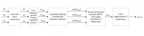
The next task is to highlight the salient regions of the DMA images that interest the human eyes, and describe the details and texture features of such regions meticulously. To this end, the Log-Gabor filter was adopted to enhance the images after PCCS conversion and their salient areas. Figure 3 clarifies the workflow of the color enhancement.
Figure 1. The workflow of quality evaluation of highly dynamic color DMA images
Figure 2. The workflow of PCCS conversion of highly dynamic color DMA images.
Figure 3. The workflow of salient area enhancement for highly dynamic color DMA images
As shown in Figure 3, the frequency domain conversion function LG of Log-Gabor filter was applied to filter the images in spatial and frequency domains, such as to extract the texture features from the images in Lab format. The weights of the salient areas in each image were calculated by:
${{W}_{VS}}=\sqrt{\begin{align} & {{\left( ifft\left[ LG({{P}_{L-fft2}}) \right] \right)}^{2}}+{{\left( ifft\left[ LG({{P}_{a-fft2}}) \right] \right)}^{2}} \\ & +{{\left( ifft\left[ LG({{P}_{b-fft2}}) \right] \right)}^{2}} \\\end{align}}$ (6)
where, PL-fft2, Pa-fft2, and Pb-fft2 are the images after Lab channel filtering and two-dimensional fast Fourier transform (FFT2) in Matlab; ifft is the inverse fast Fourier transform (IFFT) function in Matlab.
By formula (6), the weights WFpre and WRpre were obtained for the salient areas in Fpre(i, j) and Rpre(i, j). Then, the weighted images can be denoted as Fpre-W(i, j) and Rpre-W(i, j).
Considering the wide color gamut (WCG) of the highly dynamic DMA images, there are strong correlations between R, G, and B channels. Unlike the traditional quality evaluation algorithms for grayscale images, the quaternion method treats R, G, and B channels as the coefficients of the three imaginary parts i, j, and k of a quaternion, and correlates these channels cleverly by the combination in formula (7), thereby acquiring the brightness, contrast, and structural feature of highly dynamic DMA images:
$Q(p)=R(p) i+G(p) j+B(p) k$ (7)
where, Q(p) is the quaternion expression of highly dynamic DMA images at pixel p. After being processed by formula (7), the weighted images were represented as QFpre-W and QRpre-W.
Taking QFpre-W and QRpre-W as inputs, the multi-scale structure features of the images were calculated, with the aim to improve the robustness of image quality evaluation, and to reduce the influence of various factors (e.g. sampling density, and the distance between the image plane and the viewer) on the subjective evaluation of DMA images.
Let l and L be the unit scale and highest scale of the input images, respectively. Then, the number of samplings L/l=T can be controlled by adjusting the l value. Setting the sampling factor to 2, the block matching three-dimensional (BM3D) algorithm, which is based on block processing, was implemented to filter, and sample every image on the scale of l. Then, the contrast Ct and structural feature St on the t-th scale were calculated. After that, the t value was updated iteratively by t=t+1 until l≤L, and the previous steps were repeated. Note that, when l=L, the brightness BT was also recorded. Let α, β, and γ be the weight indices of contrast, brightness, and structural feature. Then, all these features can be combined by formula (8) into the final score of quality evaluation:
$Q_{s t r}=B_{T}^{\alpha} \cdot \prod_{t=1}^{T} C_{T}^{\beta} S_{T}^{\gamma}$ (8)
To convert the DMA images obtained under different imaging conditions into images under standard illumination, the images obtained through the calculation of multi-scale structure features were subject to color correction based on Retinex algorithm.
The Retinex algorithm calculates the weighted average of the value of the target pixel Q(i, j) and that of neighboring pixels. In this way, the illumination component can be removed from the image, while the reflection component is retained. The mathematical expression of Retinex algorithm is as follows:
$H(i, j)=\log Q(i, j)-\log (A(i, j) * Q(i, j))$ (9)
where, A(i, j) and Q(i, j) are normalized convolution functions for convolution operation. The value of A(i, j) can be calculated by:
$A(i, j)=\frac{1}{2 \pi \tau^{2}} \exp \left[-\frac{i^{2}+j^{2}}{2 \tau^{2}}\right]$ (10)
where, τ is the radius (Gaussian kernel size). The τ value, which determines the size of the neighborhood of the target pixel, must be selected to strike a balance between the degree of image distortion and the enhancement effect of image details. Therefore, the value of A(i, j) should satisfy the following constraint:
$\iint A(i, j) d i d j=1$ (11)
To ensure the local dynamic range of DMA images in color correction and guarantee the color reconstruction effect, the results of multiple calculations by formula (9) were subject to weighted stacking by:
$\begin{align} & {{H}_{\sum }}\left( i,j \right)= \\ & \text{ }\sum\limits_{k=\text{1}}^{K}{{{\omega }_{k}}\left[ \log Q\left( i,j \right)-\log \left( {{A}_{k}}\left( i,j \right)*Q\left( i,j \right) \right) \right]}\text{ } \\\end{align}$ (12)
where, K is the number of convolution kernels; ωk is the weight of the k-th radius; Ak(i, j) is the convolution function of the k-th radius. The weighted stacking might cause color distortion, as it increases the contrast in local areas. This problem was solved by the color correction factor below:
$\sigma(i, j)=\lambda\left\{\log [\gamma Q(i, j)]-\log \left[Q_{\Sigma}(i, j)\right]\right\}$ (13)
where, Q∑(i, j) is the stacking of the pixels in R, G, and B channels; γ=137 is the nonlinear controlled intensity coefficient; λ=38 is the gain coefficient.
Based on the multi-scale structure features, the Retinex algorithm with color correction function can be illustrated as:
$H_{\Sigma-\sigma}(i, j)=$$\sigma(i, j) \sum_{k=1}^{K} \omega_{k}\left[\log Q(i, j)-\log \left(A_{k}(i, j) * Q(i, j)\right)\right]$ (14)
The nonlocal Laplace algorithm first determines the weight matrix based on the feature similarity between the nodes of the target image and the undirected graph, and then filters the image with the nonlocal Laplace energy function, according to the results of smooth interpolation on the point cloud. The point cloud interpolation through point integration can be expressed as:
$\sum_{j \in D} W\left(-\frac{\left|p_{1}-p_{2}\right|^{2}}{4 t}\right)\left(d\left(p_{1}\right)-d\left(p_{2}\right)\right)$
$\quad+\frac{2}{\delta} \sum_{j \in D^{\prime}} \hat{W}\left(-\frac{\left|p_{1}-p_{2}\right|^{2}}{4 t}\right)\left(d\left(p_{2}\right)-d_{0}\left(p_{2}\right)\right)=0$ (15)
where, D is the set of nodes in the undirected graph; Dˊ is the set of sampled nodes in the undirected graph; d0 is the initial value of set D; δ is the positive number far smaller than 1; G and Ĝ are Gaussian weight functions satisfying:
$\frac{d}{d s} \hat{G}(s)=-G(s)=-e^{-s}$ (16)
Considering the quality requirements of 3D reconstruction and stereo vision of highly dynamic DMA images, the following strategies were adopted to solve the invalid and missing regions of single-frame color images: the color of highly dynamic DMA images was reconstructed by weighted nonlocal Laplace algorithm; the color information of neighboring pixels with highly similar depth was fully utilized to constrain and repair the redundant pixels in RGB channels and depth image of the target image.
For the given target image F, the corresponding depth image was created as the reference image R. Then, the color reconstruction is to restore the color image Fʹ∈EM×N from the sub-sample F|D. The weight matrix for the image combining color information and depth feature can be determined by:
$W(i, j)=$$\exp \left(-\frac{\left\|F(i, j)-F^{\prime}(i, j)\right\|^{2}}{b_{1}^{2}}\right) \cdot \exp \left(-\frac{\left\|R(i, j)-R^{\prime}(i, j)\right\|^{2}}{b_{2}^{2}}\right)$ (17)
where, b1 and b2 are the standard deviations to constrain the color information and depth feature. After the weight matrix W has been determined, the Laplace energy function can be expressed as:
$\min _{F} \sum_{F^{\prime}(i, j) \in D / D^{\prime}}\left(\sum_{F(i, j) \in D} W(i, j)\left[F(i, j)-F^{\prime}(i, j)\right]^{2}\right.$$+\frac{|D|}{\left|D^{\prime}\right|} \sum_{F^{\prime}(i, j) \in \Omega}\left(\sum_{F(i, j) \in \Omega} W(i, j)\left[F(i, j)-F^{\prime}(i, j)\right]^{2}\right)$ (18)
Formula (18) can be minimized by solving:
$\sum_{F(i, j) \in D}[W(i, j)+\hat{W}(i, j)]\left[F(i, j)-F^{\prime}(i, j)\right]+$
$\left(\frac{|D|}{\left|D^{\prime}\right|}-1\right)\sum_{F(i, j) \in D^{\prime}} \hat{W}(i, j)\left[F(i, j)-F_{0}(i, j)\right]=0$ (19)
where, G and Ĝ are weight matrices satisfying:
$\frac{d}{d s} \hat{W}(s)=-W(s)=-e^{-s}$ (20)
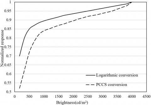
To verify the effect of PCCS conversion of highly dynamic DMA images, this paper compares the responses to PCCS conversion with those of logarithmic conversion, both of which are based on the features of human vision, under different brightness ranges. Figures 4(a) and 4(b) provide the normalized response curves under the brightness ranges of [0, 110]cd/m2 and [110, 4, 110]cd/m2, respectively. Obviously, the normalized response curves of PCCS conversion were more uniformly distributed than those of logarithmic conversion, thanks to the relatively simple conversion process. Moreover, the emission brightness of highly dynamic color DMA images simulated through PCCS conversion had a good nonlinear correlation with the perceived brightness.
(a)
(b)
Figure 4. The normalize response curves under different brightness ranges
Tables 1 and 2 compare the image quality evaluations of various algorithms on image libraries 1 and 2, respectively. The contrastive algorithms include our algorithm and several popular image quality evaluation algorithms: low dynamic range (LDR) algorithm, structural similarity index (SSIM) algorithm, multi-scale structural similarity index (MS-SSIM) algorithm, high dynamic range- video quality measure (HDR-VQM) algorithm, and convolutional neural network (CNN) algorithm. Among them, the input image of the LDR algorithm is the original image coupled with the result of visual saliency detection. The SSIM and MS-SSIM algorithms require the grayscale of the original image. The HDR-VQM algorithm needs the brightness of the original image. The CNN is an image quality evaluation and prediction model based on AlexNet.
Table 1. The image quality evaluations of various algorithms on image library 1
|
|
PSNR |
MSE |
PLCC |
KRCC |
SRCC |
|
LDR |
0.4054 |
0.8125 |
0.5034 |
0.3823 |
0.5352 |
|
SSIM |
0.5325 |
0.7303 |
0.6335 |
0.4752 |
0.6238 |
|
MS-SSIM |
0.7623 |
0.4677 |
0.8583 |
0.6969 |
0.7940 |
|
HDR-VQM |
0.9232 |
0.4533 |
0.9642 |
0.7324 |
0.8597 |
|
CNN |
0.8834 |
0.4568 |
0.8964 |
0.7106 |
0.8892 |
|
Our algorithm |
0.8945 |
0.3256 |
0.9047 |
0.8905 |
0.8346 |
Table 2. The image quality evaluations of various algorithms on image library 2
|
|
PSNR |
MSE |
PLCC |
KRCC |
SRCC |
|
LDR |
0.3564 |
0.9632 |
0.4874 |
0.4175 |
0.4294 |
|
SSIM |
0.4565 |
0.8367 |
0.6578 |
0.5752 |
0.6041 |
|
MS-SSIM |
0.6423 |
0.5897 |
0.7895 |
0.6324 |
0.7352 |
|
HDR-VQM |
0.6742 |
0.4352 |
0.8347 |
0.7596 |
0.8679 |
|
CNN |
0.9024 |
0.5322 |
0.8845 |
0.8384 |
0.8456 |
|
Our algorithm |
0.8945 |
0.3452 |
0.9146 |
0.9012 |
0.8955 |
As shown in Tables 1 and 2, the PLCC, SRCC, and KRCC of our algorithm on image library 1 were 0.9047, 0.8905, 0.8346, respectively, higher than those of LDR, SSIM, MS-SSIM, and HDR-VQM. Meanwhile, the MSEs of our algorithm on the two image libraries (0.3256 and 0.3452) were smaller than those of any other algorithm. Therefore, it can be concluded that PCCS conversion and salient area enhancement can make the quality evaluation more accurate on highly dynamic DMA images.
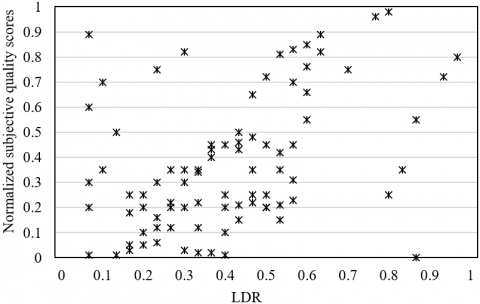
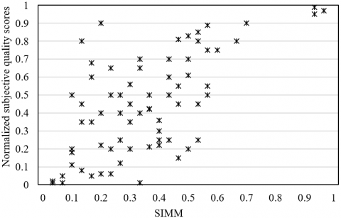
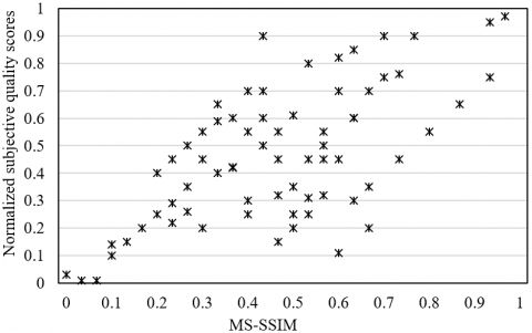
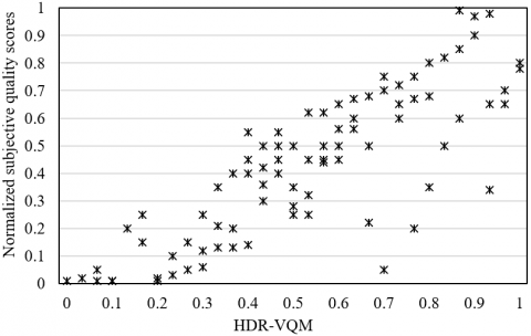
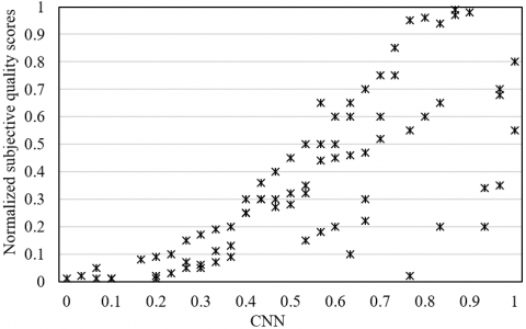
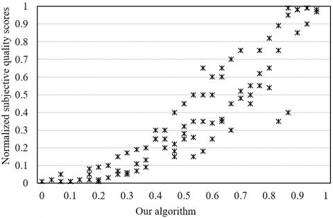
To visualize the performance of the above algorithms, the quality scores obtained by each algorithm and normalized subjective quality scores of the original images were fitted into nonlinear scatter points. As shown in Figure 5, the scatter points of our algorithm were distributed in a narrower range than those of any other algorithm, indicating the strong correlation between subjective and objective scores of highly dynamic DMA images.
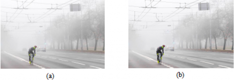
Next is to verify the correction effect of our color correction algorithm on color DMA images. A foggy image (Figure 6(a)) were selected from the image libraries as the test images. The image corrected by the traditional Retinex algorithm is given in Figure 6(b); the image corrected by Retinex + weighted stacking is given in Figure 6(c); the image corrected by Retinex + weighted stacking + color correction is given in Figure 6(d). The corrected images were evaluated against the five selected indices. The evaluation results in Table 3 show that the addition of color correction improved the index values, greatly optimizing the image quality.
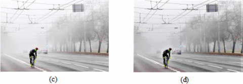
Finally, a low-illumination image (Figure 7(b)) was selected from the image libraries to verify the effect of the proposed color reconstruction algorithm on color DMA images. Figure 7(a) presents the original image of the low-illumination image under saturated light; Figure 7(c) is the image processed by the traditional Retinex algorithm; Figure 7(d) is the image reconstructed by nonlocal Laplace algorithm. Similarly, the final images were evaluated against the five selected indices. The evaluation results in Table 4 show that the index values reached the maximum after color reconstruction. Hence, our color reconstruction algorithm increased the information of image details.
(a)
(b)
(c)
(d)
(e)
(f)
Figure 5. The results of nonlinear scatter points fitted from the quality scores obtained by each algorithm
Table 3. The evaluated quality of the corrected images
|
|
PSNR |
MSE |
PLCC |
KRCC |
SRCC |
|
Original image |
0.8145 |
0.3952 |
0.8846 |
0.9012 |
0.8655 |
|
Retinex |
0.8345 |
0.3643 |
0.8843 |
0.9235 |
0.8698 |
|
Retinex + weighted stacking |
0.8678 |
0.2977 |
0.8926 |
0.9297 |
0.8745 |
|
Retinex + weighted stacking + color correction |
0.8965 |
0.2552 |
0.9034 |
0.9357 |
0.8945 |
Table 4. The evaluated quality of the original image and reconstructed image
|
|
PSNR |
MSE |
PLCC |
KRCC |
SRCC |
|
Original image |
0.8239 |
0.3547 |
0.8943 |
0.8846 |
0.8246 |
|
Image reconstructed by nonlocal Laplace algorithm |
0.8674 |
0.3146 |
0.9045 |
0.9056 |
0.8856 |
Figure 6. The original foggy image and the corrected images
Figure 7. The effect of color reconstruction
This paper explores deep into the key techniques of color management for DMA images. Firstly, five evaluation indices were chosen for highly dynamic DMA images, including PSNR, MSE, PLCC, KRCC, and SRCC, and the quality evaluation workflow was clarified. Experimental results show that, under different brightness ranges, the PCCS conversion could accurately simulate the nonlinear relationship between emission brightness and perceived brightness. In addition, the quality evaluation of our algorithm was compared with that of LDR, SSIM, MS-SSIM, HDR-VQM, and CNN, indicating that PCCS conversion and salient area enhancement can enhance the quality evaluation accuracy of highly dynamic DMA images. Furthermore, a Retinex-based color correction method was established to correct the DMA images under non-standard illumination, and a color reconstruction algorithm was developed based on nonlocal Laplace algorithm, solving the invalid and missing regions of single-frame color images. Through repeated experiments, it is proved that the color correction and color reconstruction improved the values of the evaluation indices, and greatly enriched the information of image details.
This paper was supported by the Education Department of Shaanxi Province (Grant No. 19JK0025).
[1] Chung, K.L., Hsu, T.C., Huang, C.C. (2017). Joint chroma subsampling and distortion-minimization-based luma modification for RGB color images with application. IEEE Transactions on Image Processing, 26(10): 4626-4638. https://doi.org/10.1109/TIP.2017.2719945
[2] Florea, L., Florea, C. (2019). Directed color transfer for low-light image enhancement. Digital Signal Processing, 93: 1-12. https://doi.org/10.1016/j.dsp.2019.06.014
[3] Singh, V., Dev, R., Dhar, N.K., Agrawal, P., Verma, N.K. (2018). Adaptive type-2 fuzzy approach for filtering salt and pepper noise in grayscale images. IEEE Transactions on Fuzzy Systems, 26(5): 3170-3176. https://doi.org/10.1109/TFUZZ.2018.2805289
[4] Ghodhbani, E., Kaaniche, M., Benazza-Benyahia, A. (2019). Depth-based color stereo images retrieval using joint multivariate statistical models. Signal Processing: Image Communication, 76: 272-282. https://doi.org/10.1016/j.image.2019.05.008
[5] Annaby, M.H., Rushdi, M.A., Nehary, E.A. (2018). Color image encryption using random transforms, phase retrieval, chaotic maps, and diffusion. Optics and Lasers in Engineering, 103: 9-23. https://doi.org/10.1016/j.optlaseng.2017.11.005
[6] Suryanto, Y., Ramli, K. (2017). A new image encryption using color scrambling based on chaotic permutation multiple circular shrinking and expanding. Multimedia Tools and Applications, 76(15): 16831-16854. https://doi.org/10.1007/s11042-016-3954-5
[7] Somaraj, S., Hussain, M.A. (2016). A novel image encryption technique using RGB pixel displacement for color images. 2016 IEEE 6th International Conference on Advanced Computing (IACC), Bhimavaram, pp. 275-279. https://doi.org/10.1109/IACC.2016.59
[8] Chidambaram, N., Thenmozhi, K., Rengarajan, A., Vineela, K., Murali, S., Vandana, V., Raj, P. (2018). DNA coupled chaos for unified color image encryption-a secure sharing approach. 2018 Second International Conference on Inventive Communication and Computational Technologies (ICICCT), Coimbatore, pp. 759-763. https://doi.org/10.1109/ICICCT.2018.8473288
[9] Firdous, A., ur Rehman, A., Missen, M.M.S. (2019). A highly efficient color image encryption based on linear transformation using chaos theory and SHA-2. Multimedia Tools and Applications, 78(17): 24809-24835. https://doi.org/10.1007/s11042-019-7623-3
[10] Gu, K., Jakhetiya, V., Qiao, J.F., Li, X., Lin, W., Thalmann, D. (2017). Model-based referenceless quality metric of 3D synthesized images using local image description. IEEE Transactions on Image Processing, 27(1): 394-405. https://doi.org/10.1109/TIP.2017.2733164
[11] Jakhetiya, V., Gu, K., Singhal, T., Guntuku, S.C., Xia, Z., Lin, W. (2018). A highly efficient blind image quality assessment metric of 3-D synthesized images using outlier detection. IEEE Transactions on Industrial Informatics, 15(7): 4120-4128. https://doi.org/10.1109/TII.2018.2888861
[12] Park, C., Kang, M.G. (2016). Color restoration of RGBN multispectral filter array sensor images based on spectral decomposition. Sensors, 16(5): 719. https://doi.org/10.3390/s16050719
[13] Aguilera, C., Soria, X., Sappa, A.D., Toledo, R. (2017). RGBN multispectral images: A novel color restoration approach. International Conference on Practical Applications of Agents and Multi-Agent Systems, pp. 155-163. https://doi.org/10.1007/978-3-319-61578-3_15
[14] Soria, X., Sappa, A.D., & Hammoud, R.I. (2018). Wide-band color imagery restoration for RGB-NIR single sensor images. Sensors, 18(7): 2059. https://doi.org/10.3390/s18072059
[15] Brooks, T., Mildenhall, B., Xue, T., Chen, J., Sharlet, D., Barron, J.T. (2019). Unprocessing images for learned raw denoising. 2019 IEEE/CVF Conference on Computer Vision and Pattern Recognition (CVPR), Long Beach, CA, USA, pp. 11028-11037. https://doi.org/10.1109/CVPR.2019.01129
[16] Jaroensri, R., Biscarrat, C., Aittala, M., Durand, F. (2019). Generating training data for denoising real RGB images via camera pipeline simulation. arXiv preprint arXiv:1904.08825.
[17] Chandrasekharan, R., Sasikumar, M. (2018). Fuzzy transform for contrast enhancement of nonuniform illumination images. IEEE Signal Processing Letters, 25(6): 813-817. https://doi.org/10.1109/LSP.2018.2812861
[18] Singh, M., Verma, A., Sharma, N. (2017). Bat optimization based neuron model of stochastic resonance for the enhancement of MR images. Biocybernetics and Biomedical Engineering, 37(1): 124-134. https://doi.org/10.1016/j.bbe.2016.10.006
[19] Lahdir, M., Hamiche, H., Kassim, S., Tahanout, M., Kemih, K., Addouche, S.A. (2019). A novel robust compression-encryption of images based on SPIHT coding and fractional-order discrete-time chaotic system. Optics & Laser Technology, 109: 534-546. https://doi.org/10.1016/j.optlastec.2018.08.040
[20] Berman, D., Treibitz, T., Avidan, S. (2017). Diving into haze-lines: Color restoration of underwater images. Proc. British Machine Vision Conference (BMVC), 1(2).
[21] Akkaynak, D., Treibitz, T. (2019). Sea-thru: A method for removing water from underwater images. 2019 IEEE/CVF Conference on Computer Vision and Pattern Recognition (CVPR), Long Beach, CA, USA, pp. 1682-1691. https://doi.org/10.1109/CVPR.2019.00178
[22] Li, J., Skinner, K.A., Eustice, R.M., Johnson-Roberson, M. (2017). WaterGAN: Unsupervised generative network to enable real-time color correction of monocular underwater images. IEEE Robotics and Automation Letters, 3(1): 387-394. https://doi.org/10.1109/LRA.2017.2730363
[23] Bellavia, F., Colombo, C. (2017). Dissecting and reassembling color correction algorithms for image stitching. IEEE Transactions on Image Processing, 27(2): 735-748. https://doi.org/10.1109/TIP.2017.2757262
[24] Kalra, G.S., Singh, S. (2016). Efficient digital image denoising for gray scale images. Multimedia Tools and Applications, 75(8): 4467-4484. https://doi.org/10.1007/s11042-015-2484-x
[25] Oliveira, R.B., Papa, J.P., Pereira, A.S., Tavares, J.M.R. (2018). Computational methods for pigmented skin lesion classification in images: Review and future trends. Neural Computing and Applications, 29(3): 613-636. https://doi.org/10.1007/s00521-016-2482-6