Sanaz Sagha Pirmard | Yahya Forghani*
© 2020 IIETA. This article is published by IIETA and is licensed under the CC BY 4.0 license (http://creativecommons.org/licenses/by/4.0/).
OPEN ACCESS
The Regularized Least Square (RLS) method is one of the fastest function estimation methods, but it is too sensitive to noise. Against this, ε-insensitive Support Vector Regression (ε-SVR) is robust to noise but doesn’t have a good runtime. ε-SVR supposes that the noise level is at most ε. Therefore, the center of a tube with radius ε, which is used as the estimated function, is determined in a way that the training data are located in that tube. Therefore, this method is robust to such noisy data. In this paper, to improve the runtime of ε-SVR, first, an initial estimated function is obtained using the RLS method. Then, unlike the ε-SVR model, which uses all the data to determine the lower and upper limits of the tube, our proposed method uses the initial estimated function for determining the tube and the final estimated function. Strictly speaking, the data below and above the initial estimated function are used to estimate the upper and lower limits of the tube, respectively. Thus, the number of the model constraints and, consequently, the model runtime are reduced. The experiments carried out on 15 benchmark data sets confirm that our proposed method is faster than ε-SVR, ε-TSVR and pair v-SVR, and its accuracy are comparable with that of ε-SVR, ε-TSVR and pair v-SVR.
ε-insensitive support vector regression (ε-SVR), regularized least square (RLS), runtime, function estimation
One of the most commonly used eager learning method is least-square method (LS) [1], which first was proposed by Carl Friedesh Gauss. In the LS method, the best estimated function is a function that the sum of square of the difference between the observed values and the corresponding estimated values with the estimated function is minimum. Later, on the basis of the LS method, the Regulation Least Square (RLS) method was proposed [2, 3]. The RLS uses a regularization term to reduce the complexity of estimated function and to increase its generalization ability.
ε-insensitive Support Vector Regression (ε-SVR) [4] supposes that the noise in the output variable is at most ε. Therefore, the center of a tube with radius ε, which is used as the estimated function, is determined in a way that the training data are located in that tube. Therefore, this method is robust to such noisy data. In v-SVR [5], the maximum noise level or the tube radius is considered as a model variable, which is determined in the process of solving the model. In both ε-SVR and v-SVR, the maximum noise level or the radius of the tube is considered to be constant or independent in terms of the training data characteristics. To alleviate this shortcoming, Support Vector Interval Regression Networks (SVIRNs) was proposed [6]. In SVIRNs, the upper and lower bounds of the tube are automatically determined by two independent RBF networks. In this model, the radius of the tube can change by changing the features of the training data. Therefore, SVIRNs is robust to a noise whose maximum level depends on training data features. These two networks are initialized using ε-SVR. v-Support Vector Interval Regression Networks (v-SVIRN) [7] determines the upper and lower bounds of the tube by only one neural network or one model. In Twin SVR (TSVR) [8], estimated function is determined by solving two small Quadratic Programming Problems (QPPs), while ε-SVR solves one large QPP. Solving the TSVR model needs less time than solving ε-SVR model. Later, in ε-TSVR [9], a regularization term was used to reduce the complexity of estimated function and to increase its generalization ability. The regularization term of ε-TSVR is L2-norm of the estimated function weight vector, while in L1-TWSVR model [10], L1-norm of the estimate function weight vector was used as the regularization term. L1-TWSVR is a linear programming, while ε-TSVR is a QPP. As well, the estimated function of L1-TWSVR is sparser than that of ε-TSVR. Therefore, the testing time of L1-TWSVR model is less than that of ε-TSVR. Pair v-SVR is extended version of ε-TSVR which has additional advantage of using parameter v for controlling the bounds on fraction of support vectors and error [11].
All the mentioned SVR-based methods assume that the noise distribution is symmetrical, therefore, the center of a tube which contain noisy data is used as the estimated function. In other words, the estimated function is determined in such a way that approximately half of the training data are positioned above it, and the remaining data are positioned below it. In the asymmetric v-SVR method [12], the estimated function is determined in such a way that an arbitrary number of training data are positioned above it and the remaining data are positioned below it. The size of each of these two parts of data is determined based on the prior knowledge about the noise distribution. Next, twin version of asymmetric v-SVR, i.e. asymmetric v-TSVR [13], was proposed to improve the runtime of the asymmetric v-SVR model.
Among the mentioned methods, the LS and RLS methods have the lowest runtime because each of them is an n + 1 variable problem with a close-form solution which is obtained by inverting an n × n matrix, but they are too sensitive to noisy data. Against this, SVR-based models have a good robustness against noise but do not have a good runtime because for example to solve ε-SVR problem, a quadratic programming problem with 2×n variables and linear constraints must be solved which is too time consuming. In this paper, to improve the runtime of ε-SVR, first, an initial estimated function is obtained using the RLS method. Then, unlike the ε-SVR model, which uses all training data to determine the lower and upper limits of the tube, our proposed method uses the initial estimated function for determining the tube and the final estimated function. In other words, the data below and above the initial estimated function are used to estimate the upper limit and the lower limit of the tube, respectively. Thus, the number of the model constraints and, consequently, the model runtime are reduced. The experiments carried out on 15 benchmark data sets confirm that our proposed method is faster than ε-SVR, ε-TSVR and pair v-SVR, and its accuracy are comparable with that of ε-SVR, ε-TSVR and pair v-SVR.
In continue, in Section 2, RLS and ε-SVR are introduced. Then, in Section 3, our proposed method is presented. In Section 4, the results of the experiments are presented and Section 5 provides conclusion.
2.1 RLS
Let {(x1,y1), (x2,y2), …, (xn,yn)}, be training data where $\mathrm{x} \in \mathrm{R}^{\mathrm{d}}$ is input variable and $\mathrm{y} \in \mathrm{R}$ is output variable. Suppose $\varphi(.)$ is a function which transforms data from the input space into a high-dimensional feature space. The goal is to find the function f(x)=wTφ(x)+b with the weight vector $\sum_{i=1}^{n} \alpha_{i} \varphi\left(x_{i}\right)$ and the bias b such that
$\forall i: y_{i} \cong f\left(x_{i}\right)$ (1)
For this purpose, the following model is solved:
$\min _{\alpha} \frac{1}{2}\left(\|\alpha\|^{2}+\mathrm{b}^{2}\right)+\frac{\mathrm{C}_{1}}{2} \sum_{\mathrm{i}=1}^{\mathrm{n}}\left(\mathrm{f}\left(\mathrm{x}_{\mathrm{i}}\right)-\mathrm{y}_{\mathrm{i}}\right)^{2}$ (2)
where, α=(α1, α2, …, αn)T. The first term of model (2) is intended to prevent over-fitting and to increase the generalizability. The parameter C1 controls the importance of the estimated function training error against generalization ability. Model (2) can be written as follows:
$\min _{\alpha} \frac{1}{2}\left(\|\alpha\|^{2}+\mathrm{b}^{2}\right)+\frac{\mathrm{C}_{1}}{2}\|\mathrm{K} \alpha+\mathrm{b}-\mathrm{y}\|^{2}$ (3)
where, y=(y1, y2, …, yn)T and K is a matrix of which the i-th row of j-th column, i.e. Kij, is equal to k(xj,xi)= φT(xj)φ(xi) where k(…) is a kernel function. The model (3) can be written as follows:
$\min _{\widetilde{\alpha}} L=\frac{1}{2}\|\widetilde{\alpha}\|^{2}+\frac{C_{1}}{2}\|\widetilde{\mathrm{K}} \widetilde{\alpha}-\mathrm{y}\|^{2}$ (4)
where,
$\widetilde{\alpha}=\left(\begin{array}{c}\alpha \\ \mathrm{b}\end{array}\right)$ (5)
$\widetilde{\mathrm{K}}=(\mathrm{K} \quad 1)$ (6)
At the optimal point of the model (4), we have:
$0=\frac{\partial \mathrm{L}}{\partial \widetilde{\alpha}}=\widetilde{\alpha}+\mathrm{C}_{1} \widetilde{\mathrm{K}}^{\mathrm{T}} \widetilde{\mathrm{K}} \widetilde{\alpha}-\mathrm{C}_{1} \widetilde{\mathrm{K}}^{\mathrm{T}} \mathrm{y}$ (7)
Therefore,
$\widetilde{\alpha}=C_{1}\left(\mathrm{I}+\mathrm{C}_{1} \widetilde{\mathrm{K}}^{\mathrm{T}} \widetilde{\mathrm{K}}\right)^{-1} \widetilde{\mathrm{K}}^{\mathrm{T}} \mathrm{y}$ (8)
RLS is sensitive to noise because when yi is noisy, the optimal function f(.) changes mistakenly in order to the objective function of RLS become minimum according to Eq. (2).
2.2 ε-SVR method
ε-SVR supposes that the noise level is at most ε. Therefore, the center of a tube with radius ε, which is used as the estimated function, is determined in a way that the training data are located in that tube. In other words, the function f(x)=wTφ(x)+b is determined in such a way that as much as possible,
$\forall i:-\varepsilon \leq y_{i}-f\left(x_{i}\right) \leq \varepsilon$ (9)
To do this, the following model is solved:
$\min _{\mathrm{w}, \mathrm{b}, \xi, \hat{\xi}} \frac{1}{2}\|\mathrm{w}\|^{2}+\mathrm{C} \sum_{\mathrm{i}=1}^{\mathrm{n}}\left(\xi_{\mathrm{i}}+\hat{\xi}_{\mathrm{i}}\right)$
subject to $\left\{\begin{array}{l}\mathrm{y}_{\mathrm{i}}-\mathrm{f}\left(\mathrm{x}_{\mathrm{i}}\right) \leq \varepsilon+\xi_{i}, \quad i=1,2, \ldots, n; \\ \mathrm{f}\left(\mathrm{x}_{\mathrm{i}}\right)-\mathrm{y}_{\mathrm{i}} \leq \varepsilon+\hat{\xi}_{i}, \quad i=1,2, \ldots, n; \\ \xi_{\mathrm{i}}, \hat{\xi}_{\mathrm{i}} \geq 0 \mathrm{i}=1,2, \ldots, \mathrm{n};\end{array}\right.$ (10)
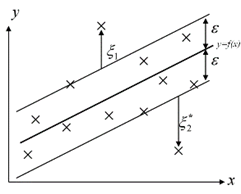
where, ξ and $\hat{\xi}$ allow outliers are not positioned outside the tube (see Figure 1). The number of outliers positioned outside the tube is controlled by the parameter C≥0.
Figure 1. The estimated function of ε-SVR for the training data represented by x signs
The dual of the model (10) is as follows:
$\max _{\alpha, \hat{\alpha}} \sum_{i=1}^{n}\left(\alpha_{i}-\hat{\alpha}_{i}\right) y_{i}-\varepsilon \sum_{i=1}^{n}\left(\hat{\alpha}_{i}+\alpha_{i}\right)$$-\frac{1}{2} \sum_{i=1}^{n} \sum_{j=1}^{n}\left(\alpha_{i}-\widehat{\alpha}_{i}\right)\left(\alpha_{j}-\widehat{\alpha}_{j}\right) k\left(x_{i}, x_{j}\right)$
snbject to $\left\{\begin{array}{l}\sum_{i=1}^{n}\left(\alpha_{i}-\hat{\alpha}_{i}\right)=0 \\ 0 \leq \alpha_{i} \leq C, \quad i=1, \ldots, n \\ 0 \leq \hat{\alpha}_{i} \leq C, \quad i=1, \ldots, n\end{array}\right.$ (11)
According to the Karush-Kuhn-Tucker (KKT) conditions [14], we have:
$\mathrm{w}=\sum_{i=1}^{\mathrm{n}}\left(\alpha_{\mathrm{i}}-\widehat{\alpha}_{\mathrm{i}}\right) \varphi\left(\mathrm{x}_{\mathrm{i}}\right)$ (12)
Therefore, the estimated function is determined according to the following formula:
$\mathrm{f}(\mathrm{x})=\mathrm{w}^{\mathrm{T}} \varphi(\mathrm{x})+\mathrm{b}=\sum_{\mathrm{i}=1}^{\mathrm{n}}\left(\alpha_{\mathrm{i}}-\widehat{\alpha}_{\mathrm{i}}\right) \mathrm{k}\left(\mathrm{x}_{\mathrm{i}}, \mathrm{x}\right)+\mathrm{b}$ (13)
where, based on the KKT conditions, the bias is determined by the following formula:
$\mathrm{b}=\left\{\begin{array}{ll}\mathrm{y}_{\mathrm{i}}-\sum_{\mathrm{j}=1}^{\mathrm{n}}\left(\alpha_{\mathrm{j}}-\widehat{\alpha}_{\mathrm{j}}\right) \mathrm{k}\left(\mathrm{x}_{\mathrm{j}}, \mathrm{x}_{\mathrm{i}}\right)-\varepsilon, & 0<\alpha_{\mathrm{i}}<\mathrm{C} \\ \mathrm{y}_{\mathrm{i}}-\sum_{\mathrm{j}=1}^{\mathrm{n}}\left(\alpha_{\mathrm{j}}-\widehat{\alpha}_{\mathrm{j}}\right) \mathrm{k}\left(\mathrm{x}_{\mathrm{j}}, \mathrm{x}_{\mathrm{i}}\right)+\varepsilon, & 0<\widehat{\alpha}_{\mathrm{i}}<\mathrm{C}\end{array}\right.$ (14)
The RLS have the good runtime, but it is sensitive to noisy data. Against this, ε-SVR model-based models are robust to noise but do not have a good runtime. In this paper, to improve the runtime of ε-SVR, first, an initial estimated function is obtained using the RLS method. Then, unlike the ε-SVR model, which uses all training data to determine the lower and upper limits of the tube, our proposed method uses the initial estimated function for determining the tube and the final estimated function. In other words, the data below and above the initial estimated function are used to estimate the upper and the lower limits of the tube, respectively. Thus, the number of the model constraints and, consequently, the model runtime are reduced.
Let $\mathrm{f}(\mathrm{x})=\sum_{\mathrm{i}=1}^{\mathrm{n}} \alpha_{\mathrm{i}} \mathrm{k}\left(\mathrm{x}_{\mathrm{i}}, \mathrm{x}\right)+\mathrm{b}$ be initial estimated function obtained by using the RLS model based on the training data {(x1,y1), (x2,y2), …, (xn,yn)}. If f(xi )≤0 then (xi,yi) is a point below the function f(.); otherwise, (xi,yi) is a point above the function f(.). Let Ia be the index of the training data above the function f, and Ib be the index of the training data below the function f, and |Ia|+|Ib|=n. Our proposed model for determining a tube with the radius ε and the center $\tilde{f}(x)=w^{T} \varphi(x)+b$ is as follows:
$\operatorname{Min}_{\mathbf{w}, \mathbf{b}, \bar{\xi}} \frac{1}{2}\|\mathbf{w}\|^{2}+\mathrm{C}_{2} \sum_{i=1}^{\mathrm{n}} \xi_{\mathrm{i}}$
subject to $\left\{\begin{array}{l}\mathrm{y}_{\mathrm{i}}-\tilde{\mathrm{f}}\left(\mathrm{x}_{\mathrm{i}}\right) \leq \varepsilon+\xi_{\mathrm{i}}, \mathrm{i} \in \mathrm{I}_{\mathrm{a}} \\ \tilde{\mathrm{f}}\left(\mathrm{x}_{\mathrm{i}}\right)-\mathrm{y}_{\mathrm{i}} \leq \varepsilon+\xi_{\mathrm{i}}, \mathrm{i} \in \mathrm{I}_{\mathrm{b}} \\ \xi_{\mathrm{i}} \geq 0, \quad \mathrm{i}=1,2, \ldots, \mathrm{n}\end{array}\right.$ (15)
where, ξ allows outliers are not positioned outside the tube. The number of outliers positioned outside the tube is controlled by the parameter C2. Unlike ε-SVR which uses all training data to determine the lower and upper bounds of the tube, in our proposed model, only the upper half of the training data is used to determine the upper limit of the tube, and also only the lower half of the training data is used to determine the lower limit of the tube. The upper half and lower half of training data are determined based on the initial estimated function obtained by the RLS. The Lagrange function of the model (15) is as follows:
$\mathrm{L}=\frac{1}{2}\|\mathrm{w}\|^{2}+\mathrm{C} \sum_{\mathrm{i}=1}^{\mathrm{n}} \xi_{\mathrm{i}}$
$-\sum_{\mathrm{i} \in \mathrm{I}_{\mathrm{a}}} \alpha_{\mathrm{i}}\left(\varepsilon+\xi_{\mathrm{i}}-\mathrm{y}_{\mathrm{i}}+\mathrm{w}^{\mathrm{T}} \varphi\left(\mathrm{x}_{\mathrm{i}}\right)+\mathrm{b}\right)$
$-\sum_{\mathrm{i} \in \mathrm{I}_{\mathrm{b}}} \alpha_{\mathrm{i}}\left(\varepsilon+\xi_{\mathrm{i}}+y_{\mathrm{i}}-\mathrm{w}^{\mathrm{T}} \varphi\left(\mathrm{x}_{\mathrm{i}}\right)-\mathrm{b}\right)-\sum_{\mathrm{i}=1}^{\mathrm{n}} \gamma_{\mathrm{i}} \xi_{\mathrm{i}}$ (16)
where, γi and αi are Lagrange coefficients. At the optimal point of the model (15) we have:
$\frac{\partial \mathrm{L}}{\partial \mathrm{w}}=0 \rightarrow \mathrm{w}=\sum_{\mathrm{i} \in \mathrm{I}_{\mathrm{a}}} \alpha_{\mathrm{i}} \varphi\left(\mathrm{x}_{\mathrm{i}}\right)-\sum_{\mathrm{i} \in \mathrm{I}_{\mathrm{b}}} \alpha_{\mathrm{i}} \varphi\left(\mathrm{x}_{\mathrm{i}}\right)$ (17)
$\frac{\partial \mathrm{L}}{\partial \mathrm{b}}=0 \rightarrow \sum_{\mathrm{i} \in \mathrm{I}_{\mathrm{a}}} \alpha_{\mathrm{i}}-\sum_{\mathrm{i} \in \mathrm{I}_{\mathrm{b}}} \alpha_{\mathrm{i}}=0$ (18)
$\frac{\partial \mathrm{L}}{\partial \xi}=0 \rightarrow \alpha_{\mathrm{i}}=\mathrm{C}_{2}-\gamma_{\mathrm{i}}, \quad \mathrm{i}=1,2, \ldots, \mathrm{n}$ (19)
$\mathrm{y}_{\mathrm{i}}-\mathrm{w}^{\mathrm{T}} \varphi\left(\mathrm{x}_{\mathrm{i}}\right)-\mathrm{b} \leq \varepsilon+\xi_{\mathrm{i}}, \quad \mathrm{i} \in \mathrm{I}_{\mathrm{a}}$ (20)
$\mathrm{w}^{\mathrm{T}} \varphi\left(\mathrm{x}_{\mathrm{i}}\right)+\mathrm{b}-\mathrm{y}_{\mathrm{i}} \leq \varepsilon+\xi_{\mathrm{i}}, \quad \mathrm{i} \in \mathrm{I}_{\mathrm{b}}$ (21)
$\alpha_{\mathrm{i}}\left(\varepsilon+\xi_{\mathrm{i}}-y_{\mathrm{i}}+\mathrm{w}^{\mathrm{T}} \varphi\left(\mathrm{x}_{\mathrm{i}}\right)+\mathrm{b}\right)=0, \quad \mathrm{i} \in \mathrm{I}_{\mathrm{a}}$ (22)
$\alpha_{i}\left(\varepsilon+\xi_{i}+y_{i}-w^{T} \varphi\left(x_{i}\right)-b\right)=0, \quad i \in I_{b}$ (23)
$\gamma_{i} \xi_{i}=0, \quad i=1,2, \ldots, n$ (24)
$\xi_{\mathrm{i}}, \alpha_{\mathrm{i}}, \gamma_{\mathrm{i}} \geq 0, \quad \mathrm{i}=1,2, \ldots, \mathrm{n}$ (25)
By substituting Eq. (17) to Eq. (24) into the Lagrange function, this function is simplified as follows:
$\mathrm{L}=\sum_{\mathrm{i} \in \mathrm{I}_{\mathrm{o}}} \alpha_{\mathrm{i}} \mathrm{y}_{\mathrm{i}}-\sum_{\mathrm{i} \in \mathrm{I}_{\mathrm{u}}} \alpha_{\mathrm{i}} \mathrm{y}_{\mathrm{i}}-\varepsilon \sum_{\mathrm{i}=1}^{\mathrm{n}} \alpha_{\mathrm{i}}$
$-\frac{1}{2}\left(\sum_{i \in I_{0}} \sum_{j \in I_{0}} \alpha_{i} \alpha_{i} k\left(x_{i}, x_{j}\right)+\sum_{i \in I_{u}} \sum_{j \in I_{u}} \alpha_{i} \alpha_{j} k\left(x_{i}, x_{j}\right)-2 \sum_{i \in I_{0}} \sum_{j \in I_{u}} \alpha_{i} \alpha_{j} k\left(x_{i}, x_{i}\right)\right)$ (26)
In addition, according to Eq. (19), and since αi,γi≥0, we have:
$0 \leq \alpha_{\mathrm{i}} \leq \mathrm{C}_{2}, \quad \mathrm{i}=1,2, \ldots, \mathrm{n}$ (27)
Therefore, the dual of the model (15) is as follows:
$\max _{\alpha} \sum_{i \in I_{a}} \alpha_{i} y_{i}-\sum_{i \in I_{b}} \alpha_{i} y_{i}-\varepsilon \sum_{i=1}^{n} \alpha_{i}$
$-\frac{1}{2}\left(\sum_{i \in I_{a}} \sum_{j \in I_{a}} \alpha_{i} \alpha_{j} k\left(x_{i}, x_{j}\right)+\sum_{i \in I_{b}} \sum_{j \in I_{b}} \alpha_{i} \alpha_{j} k\left(x_{i}, x_{j}\right)\right.$
$\left.-2 \sum_{i \in I_{a}} \sum_{j \in I_{b}} \alpha_{i} \alpha_{j} k\left(x_{i}, x_{j}\right)\right)$
subject to $\left\{\begin{array}{l}\sum_{i \in I_{a}} \alpha_{i}-\sum_{i \in I_{b}} \alpha_{i}=0 \\ 0 \leq a_{i} \leq C_{2}, \quad i=1,2, \ldots, n\end{array}\right.$ (28)
If we define:
$\beta_{i}=\left\{\begin{array}{ll}\alpha_{i}, & i \in I_{0} \\ -\alpha_{i}, & i \in I_{u}\end{array}\right.$ (29)
then, the model (28) can be written as follows:
$\max _{\beta} \sum_{i=1}^{n} \beta_{i} y_{i}-\varepsilon\left(\sum_{i \in I_{a}} \beta_{i}-\sum_{i \in I_{b}} \beta_{i}\right)$$-\frac{1}{2} \sum_{i=1}^{n} \sum_{j=1}^{n} \beta_{i} \beta_{j} k\left(x_{i}, x_{j}\right)$
subject to $\left\{\begin{array}{l}\sum_{i=1}^{n} \beta_{i}=0 \\ 0 \leq \beta_{i} \leq C_{2}, \quad i \in I_{a} \\ -C_{2} \leq \beta_{i} \leq 0, \quad i \in I_{b}\end{array}\right.$ (30)
which is a convex quadratic programming problem. After solving the model (30) and obtaining the optimal value of $\beta$, the optimal values of $\alpha$ can be determined using Eq. (29). Given Eq. (22), for each $\mathrm{i} \in \mathrm{I}_{\mathrm{a}}$, if αi>0 then
$y_{i}-w^{T} \varphi\left(x_{i}\right)-b=\varepsilon+\xi_{i}$ (31)
and according to Eq. (19), if αi<C2 then
$\gamma_{i}>0$ (32)
Then, according to Eq. (24), we have:
$\xi_{i}=0$ (33)
Thus, for each $\mathrm{i} \in \mathrm{I}_{\mathrm{a}}$, if 0<αi<C2, the bias can be obtained from the following equation:
$\mathrm{b}=y_{\mathrm{i}}-\mathrm{w}^{\mathrm{T}} \varphi\left(\mathrm{x}_{\mathrm{i}}\right)-\varepsilon$ (34)
According to Eq. (23), for each i $\mathrm{i} \in \mathrm{I}_{b}$, if αi>0, then
$-y_{i}+w^{T} \varphi\left(x_{i}\right)+b=\varepsilon+\xi_{i}$ (35)
and according to Eq. (19), if αi<C2, then
$\gamma_{i}>0$ (36)
Then, according to Eq. (24), we have:
$\xi_{\mathrm{i}}=0$ (37)
Thus, for each $\mathrm{i} \in \mathrm{I}_{\mathrm{u}}$, if 0<αi<C2, the bias can be obtained from the following equation:
$\mathrm{b}=\varepsilon+\mathrm{y}_{\mathrm{i}}-\mathrm{w}^{\mathrm{T}} \varphi\left(\mathrm{x}_{\mathrm{i}}\right)$ (38)
According to Eq. (17), the optimal hyperplane or estimated function is as follows:
$f(x)=w^{T} \varphi(x)+b$$=\mathrm{b}+\sum_{\mathrm{i} \in \mathrm{I}_{\mathrm{a}}} \alpha_{\mathrm{i}} \mathrm{k}\left(\mathrm{x}, \mathrm{x}_{\mathrm{i}}\right)-\sum_{\mathrm{i} \in \mathrm{I}_{\mathrm{b}}} \alpha_{\mathrm{i}} \mathrm{k}\left(\mathrm{x}, \mathrm{x}_{\mathrm{i}}\right)$$=\mathrm{b}+\sum_{i=1}^{\mathrm{n}} \beta_{\mathrm{i}} \mathrm{k}\left(\mathrm{x}, \mathrm{x}_{\mathrm{i}}\right)=\mathrm{b}+\sum_{\mathrm{i} \in \mathrm{SV}} \beta_{\mathrm{i}} \mathrm{k}\left(\mathrm{x}, \mathrm{x}_{\mathrm{i}}\right)$ (39)
where, $\mathrm{SV}=\left\{\mathrm{i} \mid \beta_{\mathrm{i}} \neq 0\right\}$ is called support vector set.
In this section, our proposed method is compared with ε-SVR [4], ε-TSVR [9] and pair v-SVR [11] using 15 benchmark data sets of the UCI repository. The characteristics of these data sets are in accordance with Table 1. The kernel function used in each regression method is Gaussian kernel function. For each data set, the optimal values of the parameters C1,C2,C3,C4 were selected from the set {0,0.01,…,100}, the optimal value of the parameter ε1=ε2=ε was selected from the set {0,0.1}, and the optimal value of the parameter σ was selected from the set {0.1,0.2,…,100} by using the grid search mechanism. These optimal values were reported in Table 2. The RMSE and runtime of each method for the best values of their parameters are according to Table 3 and Table 4, respectively. To calculate RMSE, 10-fold cross validation was used. As it can be seen, the RMSE of our proposed method is competitive with the three other methods and the run time of our proposed method is much less than that of ε-SVR and less than that of ε-TSVR and pair v-SVR. The reason is that in our proposed method instead of solving the constrained quadratic programming problem (11) with 2×n variables, two smaller problems, i.e. the unconstrained quadratic programming problem (2) with n + 1 variables, and then the constrained quadratic programming problem (30) with n variables are solved. Also, in each of ε-TSVR and pair v-SVR, two constrained quadratic programming problem problems with variables are solved. Solving the mentioned unconstrained quadratic problem is faster than the mentioned constrained quadratic problems of the same size. It should be noted that, each problem was solved using MATLAB2015 on a computer of 8GbRAM and 2.20GHz CPU. The quadprog function and the interior-point-convex algorithm were used to solve each constrained quadratic model.
Table 1. Characteristics of 15 UCI datasets
|
No. |
Dataset |
Application |
#Instance |
#Feature |
|
1 |
Pyrimidine |
Regression |
74 |
27 |
|
2 |
Triazines |
Regression |
186 |
61 |
|
3 |
Bodyfat |
Regression |
252 |
14 |
|
4 |
Haberman |
Classification |
306 |
4 |
|
5 |
Yacht Hydrodynamics |
Regression |
308 |
7 |
|
6 |
ionosphere |
Classification |
351 |
34 |
|
7 |
Housing |
Regression |
506 |
14 |
|
8 |
Pima Indians Diabetes |
Classification |
768 |
8 |
|
9 |
Concrete Compressive Strength |
Regression |
1030 |
9 |
|
10 |
Mg |
Regression |
1385 |
7 |
|
11 |
banknote authentication |
Classification |
1372 |
5 |
|
12 |
Abalone |
Regression |
4177 |
8 |
|
13 |
Wine |
Regression |
4898 |
12 |
|
14 |
Wisconsin Breast Cancer |
Classification |
569 |
32 |
|
15 |
Forest Fires |
Regression |
517 |
13 |
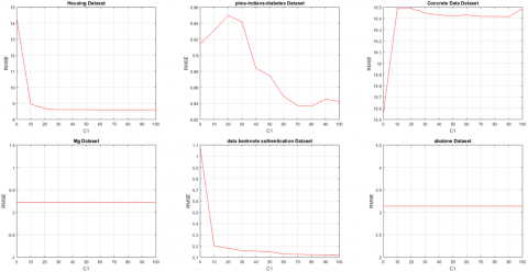
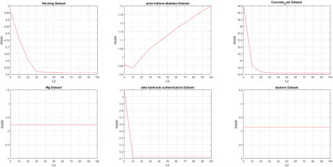
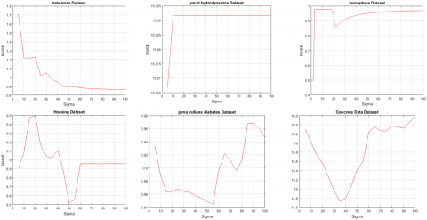
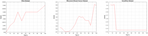
Note that determination of appropriate values for the parameters of a model is a challenging issue which can be estimated using a validation set or based on prior knowledge which may not be available for each dataset. The Figures 2, 3 and 4 show the sensitivity of RMSE of our proposed method to the parameters C1, C2, and σ, respectively. According to Figure 2, for each dataset except “Concrete” dataset, the best RMSE can be obtained by a large value of C1. Moreover, the sensitivity of RMSE of our proposed method to the parameter C1 for “Concrete” dataset is small. According to Figure 3, the best RMSE can be obtained by a large value of C2 for some datasets and the best RMSE can be obtained by a small value of C2 for the others. But, as it can be seen, the RMSE is not too sensitive to a wide range of values of C2. For example, the sensitivity of MSE of our proposed method to the parameter C2 for “Triazines” dataset is about 0.004 for the range [0,100]. According to Figure 4, the RMSE is also not too sensitive to a wide range of the values of σ. For example, the sensitivity of MSE of our proposed method to the parameter σ for “Triazines” dataset is about 0.16 for its whole range, and about 0.01 for the range [20,100].
Table 2. The best parameters of our proposed method with the lowest RMSE
|
Dataset |
σ |
C1 |
C2 |
|
Pyrimidine |
63.4 |
100 |
100 |
|
Triazines |
28.3 |
100 |
100 |
|
Bodyfat |
100 |
100 |
20 |
|
Haberman |
100 |
100 |
100 |
|
Yacht Hydrodynamics |
2 |
0.01 |
100 |
|
ionosphere |
1.4 |
50 |
1 |
|
Housing |
50 |
0.01 |
100 |
|
Pima Indians Diabetes |
49.4 |
100 |
1 |
|
Concrete Compressive Strength |
38 |
0.01 |
100 |
|
Mg |
2 |
0.01 |
100 |
|
Banknote authentication |
1.2 |
100 |
10 |
|
Abalone |
100 |
100 |
100 |
|
Wine |
1 |
100 |
100 |
|
Wisconsin Breast Cancer |
20.1 |
20 |
1 |
|
Forest Fire |
59.3 |
100 |
1 |
Table 3. The mean and standard deviation of RMSE of our proposed method, ε-SVR, ε-TSVR and pair v-SVR
|
Dataset |
ε-SVR |
ε-TSVR |
pair v-SVR |
proposed |
|
Pyrimidine |
0.0842± 0.0593 |
0.0656± 0.0471 |
0.0675±0 .0367 |
0.1180± 0.0615 |
|
Triazines |
0.1503± 0.0338 |
0.1362± 0.0434 |
0.1456± 0.0457 |
0.1512± 0.0332 |
|
Bodyfat |
4.7757± 0.8102 |
8.1441± 2.1848 |
7.6785± 1.5767 |
6.2215± 1.4876 |
|
Haberman |
0.8664± 0.1086 |
0.8775± 0.1395 |
0.8452± 0.1065 |
0.8615± 0.1055 |
|
Yacht Hydrodynamics |
10.9085± 1.2578 |
10.3360± 1.8207 |
10.5678± 1.5342 |
9.6190± 0.9907 |
|
Ionosphere |
0.5148± 0.1096 |
0.5022± 0.1283 |
0.4322± 0.1164 |
0.4354± 0.1279 |
|
Housing |
6.7392± 2.1573 |
8.9263± 3.5525 |
7.5678± 3.4234 |
8.5130± 3.3002 |
|
Pima Indians Diabetes |
0.9112± 0.0640 |
0.9871± 0.0033 |
0.9454± 0.0197 |
0.8425± 0.0946 |
|
Concrete Compressive Strength |
13.9188± 6.8642 |
14.6849± 7.1039 |
13.7545± 6.7433 |
14.6370± 5.2094 |
|
Mg |
0.1014± 0.0123 |
0.1113± 0.0156 |
0.0945± 0.0154 |
0.0999± 0.0134 |
|
Banknote authentication |
0.0857± 0.0184 |
0.0768± 0.0183 |
0.0956± 0.0224 |
0.1178± 0.0209 |
|
Abalone |
2.0999± 0.6538 |
2.1265± 0.6173 |
2.0451± 0.9835 |
3.1384± 0.9881 |
|
Wine |
0.8637± 0.0660 |
0.8685± 0.0576 |
0.8621± 0.0452 |
0.8601± 0.0355 |
|
Wisconsin Breast Cancer |
1.8819± 0.5168 |
1.8847± 0.5224 |
1.8664± 0.4767 |
1.8703± 0.4350 |
|
Forest Fires |
0.1974± 0.2502 |
0.1288± 0.2810 |
0.1198± 0.2576 |
0.1250± 0.2746 |
Table 4. The runtime of our proposed method, ε- SVR, ε-TSVR and pair v-SVR (seconds)
|
Dataset |
ε-SVR |
ε-TSVR |
pair v-SVR |
proposed |
|
Pyrimidine |
0.41 |
0.29 |
0.35 |
0.12 |
|
Triazines |
3.44 |
2.12 |
2.87 |
1.71 |
|
Bodyfat |
5.69 |
0.71 |
1.75 |
0.28 |
|
Haberman |
8.34 |
0.78 |
2.76 |
0.43 |
|
Yacht Hydrodynamics |
9.79 |
0.64 |
3.65 |
0.26 |
|
ionosphere |
9.12 |
4.20 |
6.43 |
3.08 |
|
Housing |
33.94 |
2.06 |
9.34 |
0.77 |
|
Pima Indians Diabetes |
40.85 |
13.45 |
21.67 |
12.34 |
|
Concrete Compressive Strength |
144.2 |
40.79 |
31.43 |
38.32 |
|
Mg |
187.02 |
10.26 |
49.45 |
4.84 |
|
Banknote authentication |
252.38 |
11.82 |
51.43 |
11.70 |
|
Abalone |
14202.98 |
199.51 |
199.51 |
54.07 |
|
Wine |
3906.94 |
1384.58 |
2232.32 |
920.94 |
|
Wisconsin Breast Cancer |
2.87 |
1.92 |
2.02 |
1.53 |
|
Forest Fires |
17.81 |
3.70 |
5.21 |
2.51 |
Figure 2. The sensitivity of our proposed method to the parameter C1 for the best C2 and σ reported in Table 2
Figure 3. The sensitivity of our proposed method to the parameter C2 for the best C1 and σ reported in Table 2
Figure 4. The sensitivity of our proposed method to the parameter σ for the best C1 and C2 reported in Table 2
The RLS method is one of the fastest methods for function estimation because it is an n + 1 variable problem with a close-form solution which is obtained by inverting an n × n matrix. The RLS has a high sensitivity to noisy data. Against this, ε-SVR has a good resistance against noise, but its runtime is not as good as the RLS runtime, because in order to solve the dual ε-SVR, we need to solve a quadratic programming problem with 2×n variables and linear constraints. ε-SVR supposes that the noise in the output variable is at most ε. Therefore, the center of a tube with radius ε, which is used as the estimated function, is determined in a way that the training data are located in that tube. Therefore, this method is robust to such noisy data. In this paper, to improve the runtime of ε-SVR, first, an initial estimated function was obtained using the RLS method. Then, unlike ε-SVR which uses all data to determine the lower and upper limits of the tube, our proposed method used the initial estimated function for determining the tube and the final estimated function. Strictly speaking, the data below and above the initial estimated function were used to estimate the upper and lower limits of the tube, respectively. Thus, the number of the model constraints and, consequently, the model runtime were reduced.
Our proposed method runtime is also lower than that of ε-TSVR and pair v-SVR because in each of ε-TSVR and pair v-SVR, two quadratic programming problems with n-variables and linear constraints are solved, while in our proposed method, an unconstrained quadratic programming problem with n+1 variables and a close form solution, and then, a quadratic programming problem with n-variables and linear constraints are solved. Solving an unconstrained quadratic programming problem is faster than a constrained quadratic programming problem of the same size. Our experiments on 15 benchmark dataset confirm that our proposed method is faster than ε-SVR, ε-TSVR and pair v-SVR, and its accuracy is comparable with the ε-SVR, ε-TSVR and pair v-SVR.
|
xi |
i-th training data |
|
yi |
Class label of i-th training data |
|
$\xi_{\mathrm{i}}, \hat{\xi}_{\mathrm{i}}$ |
Slack variables for i-th training data |
|
n |
The number of training data |
|
w |
Weight vector of htperplane |
|
b |
Bias of hyperplane |
|
$\alpha_{i}, \widehat{\alpha}_{i}$ |
Lagrange coefficients for i-th training data |
|
φ(.) |
A function which map data from the input space into a high-dimensional feature space |
|
k(.,.) |
Kernel function |
|
σ |
Hyper-parameter of Gaussian kernel function |
|
C1,C2,C3,C4 |
Hyper-parameters of models to control penalty terms |
|
ε |
Size of tube |
[1] Otto Bretscher, S. (1997). Linear Algebra with Applications. USA: Prentice-Hall International Inc.
[2] Tibshirani, R. (1996). Regression shrinkage and selection via the lasso. Journal of the Royal Statistical Society. Series B (Methodological), 58(1): 267-288. https://doi.org/10.1111/j.2517-6161.1996.tb02080.x
[3] Zou, H., Hastie, T. (2005). Regularization and variable selection via the elastic net. Journal of the Royal Statistical Society: Series B (Statistical Methodology), 67(2): 301-320. https://doi.org/10.1111/j.1467-9868.2005.00503.x
[4] Vapnik, V. (2013). The nature of statistical learning theory. Springer Science & Business Media.
[5] Schölkopf, B., Smola, A.J., Williamson, R.C., Bartlett, P.L. (2000). New support vector algorithms. Neural Computation, 12(5): 1207-1245. https://doi.org/10.1162/089976600300015565
[6] Jeng, J.T., Chuang, C.C., Su, S.F. (2003). Support vector interval regression networks for interval regression analysis. Fuzzy Sets and Systems, 138(2): 283-300. https://doi.org/10.1016/S0165-0114(02)00570-5
[7] Hao, P.Y. (2009). Interval regression analysis using support vector networks. Fuzzy Sets and Systems, 160(17): 2466-2485. https://doi.org/10.1016/j.fss.2008.10.012
[8] Peng, X. (2010). TSVR: An efficient twin support vector machine for regression. Neural Networks, 23(3): 365-372. https://doi.org/10.1016/j.neunet.2009.07.002
[9] Shao, Y.H., Zhang, C.H., Yang, Z.M., Jing, L., Deng, N.Y. (2013). An ε-twin support vector machine for regression. Neural Computing and Applications, 23(1): 175-185. https://doi.org/10.1007/s00521-012-0924-3
[10] Peng, X., Xu, D., Kong, L.Y., Chen, D.J. (2016). L1-norm loss based twin support vector machine for data recognition. Information Sciences, 340-341: 86-103. https://doi.org/10.1016/j.ins.2016.01.023
[11] Hao, P.Y. (2017). Pair v-SVR: A novel and efficient pairing nu-support vector regression algorithm. IEEE Transactions on Neural Networks and Learning Systems, 28(11): 2503-2515. https://doi.org/10.1109/TNNLS.2016.2598182
[12] Huang, X., Shi, L., Pelckmans, K., Suykens, J.A.K. (2014). Asymmetric ν-tube support vector regression. Computational Statistics & Data Analysis, 77: 371-382. https://doi.org/10.1016/j.csda.2014.03.016
[13] Xu, Y., Li, X.Y., Pan, X.L., Yang, Z.J. (2017). Asymmetric ν-twin support vector regression. Neural Computing and Applications, 30: 1-16. https://doi.org/10.1007/s00521-017-2966-z
[14] Kuhn, H.W., Tucker, A.W. (2014). Nonlinear programming, in Traces and emergence of nonlinear programming. Springer, pp. 247-258.