Real-Time Object Detection for Forklift Automated Guided Vehicles Using Deep Learning

The development of Automated Guided Vehicles (AGVs) represents a significant technological milestone. AGVs, which are intelligent robots used for automatic material handling in industrial settings and ports [1], have seen their traditional methods overshadowed by modern technologies such as deep learning and advanced sensors. These traditional methods are often time-consuming, error-prone, and unsafe. Improving automation is essential for industrial competitiveness, operational efficiency, and sustainability. AGVs face challenges such as misclassification, low inference speed, and potential collisions [2, 3]. Effective real-time object detection depends on accuracy and speed [4, 5], with many detection networks focusing on accuracy while neglecting computational complexity. Consequently, enhancing AGV performance is a key research area [6].

Recent advances in Convolutional Neural Networks (CNNs) [7, 8] offer promising solutions to complex computer vision problems [9], improving speed and accuracy compared to older methods. However, real-time neural networks require substantial computing power, which poses challenges when integrating them with embedded systems such as Arduino and Raspberry Pi [10]. The RetinaNet model, featuring multiple convolutional layers [11], and the Faster Region Convolutional Neural Networks (RCNN) model, which utilizes a Region Proposal Network for feature acquisition, represent notable object detection approaches [12]. However, these methods often suffer from slow detection speeds.

In contrast, the You Only Look Once (YOLO) model offers rapid inference with single-stage detection [13]. YOLOv3, widely adopted for its efficiency, employs Darknet-53 for direct predictions without needing additional proposal generation. Despite its advancements, YOLOv3 struggles with detecting small, densely distributed, or occluded objects under varying lighting conditions [5, 14]. Real-time communication protocols, such as Web Real-Time Communication (WebRTC), offer low latency but face limitations in certain applications [15, 16]. To address these issues, an improvement to the YOLOv3 model is proposed, along with constructing and applying a smart control architecture for AGVs to enable object detection in autonomous driving environments. The developed model achieves a dual-directional improvement in object detection accuracy and speed during autonomous driving. The system operates in real-time using the Secure Shell (SSH) protocol for communication, ensuring efficient and secure data exchange between the hardware and software components. The key contributions of this study are summarized as follows:

(1) Design and implementation of an integrated hardware-software AGV system using Raspberry Pi 4 for real-time object detection and autonomous control.

(2) Development of an enhanced YOLOX-based model to improve object detection accuracy in complex environments.

(3) Utilization of mix-up and label smoothing techniques to augment the dataset, improve generalization, and reduce classification errors.

(4) Application of Adaptive Spatial Feature Fusion (ASFF) with adaptive weights (α, β, γ) to improve multi-scale feature integration and small object detection.

(5) Experimental validation of the system’s real-time performance in dynamic indoor environments under varied lighting and obstacle scenarios.

The structure of this paper is organized as follows: Section 2 reviews related work, Section 3 presents the methodology, Section 4 describes the monitoring and control system and its integration with the Forklift AGV, Section 5 summarizes the results and evaluation metrics, Section 6 discusses the findings, and Section 7 concludes the paper.

The proposed system was developed through a structured methodology encompassing hardware configuration, software implementation, and full system integration into an AGV prototype. This section outlines the experimental setup and implementation details across both hardware and software domains.

3.1 Hardware configuration

The hardware framework consists of two main controllers:

• Main Controller: A high-performance computing unit configured with an Intel® Core™ i7-11800H (11th Gen) processor @ 2.30 GHz, 32 GB of memory, and 512 GB of NVMe SSD storage, used primarily for object detection and decision-making tasks.

• Sub-controller (Raspberry Pi 4): Responsible for data acquisition and basic control tasks. It is equipped with a Cortex-A72 quad-core processor, 8 GB RAM, and dual-band wireless capability. The Pi Camera module captures 5 MP images and streams real-time video at 1080p/30 FPS to the main controller for further processing. Additional components include:

• Ultrasonic Sensor (HC-SR04): Used for obstacle detection within a range of 2 cm to 400 cm. The sensor is interfaced with the Raspberry Pi GPIO pins and operates through a voltage divider to ensure compatibility with 3.3V logic.

• Relay Modules: Used for controlling actuator responses in the prototype. All components were mounted onto a Forklift AGV robot. This setup enables real-time testing of object detection, classification, and motion control capabilities in a semi-structured environment.

3.2 Software implementation

The software environment was developed using Python 3.11 and OpenCV2 [24], in conjunction with the YOLOX object detection framework. Model training and testing were performed using the Pascal VOC dataset. VOC 2012 includes 11,530 images containing 27,450 annotated objects, and VOC 2007 consists of 9,963 images with a total of 24,640 labeled objects [25]. Both VOCs contain eleven object classes relevant to AGV operations. Input images were resized to 608×608 pixels, and bounding boxes were normalized accordingly. The training process utilized Darknet53 as the backbone network within a CUDA-accelerated PyTorch environment, leveraging pre-trained weights for optimized convergence. The model’s effectiveness was assessed using the mAP metric and inference latency to ensure real-time viability on the embedded system.

3.3 System integration

Following hardware and software development, the full system was deployed on the Forklift AGV prototype. This integration facilitated the real-time transfer of data from sensors and cameras to the detection model, allowing the AGV to recognize, classify, and respond to objects and activities autonomously. The systems behavior was evaluated in various indoor scenarios to evaluate detection accuracy, decision speed, and system robustness.

3.4 Object detection

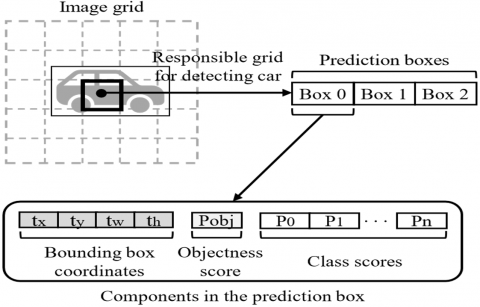
In recent years, deep learning (DL) methods have been widely applied to object detection, as they can extract fine-grained visual features and progressively construct more abstract semantic representations. These DL-based methods enable a hierarchical representation of data, enhancing the object detection process. For multi-classification tasks, DL-based object detection outperforms conventional detection methods in terms of speed, accuracy, and robustness. The ongoing advancement of neural networks using convolutions (CNNs) [8] has significantly advanced object detection, with contemporary deep CNN-based object detectors such as SSD, R-CNN, and YOLO being essential to this advancement [26]. To efficiently extract features, these detectors employ DL methods. Nevertheless, CNNs require constructing their network structure and optimizing weight parameters through training [7, 14]. YOLOv3 is an improved variant of YOLO and YOLOv2. This network directly uses a single feed-forward method to estimate class probabilities and bounding box offsets from complete images CNN, eliminating the need to generate region proposals or sample features [27]. In YOLOv3, the input is divided into grid cells of size S×S. It is the grid cell's responsibility to detect an object when its center point is inside its borders. Every cell in the model computes the object scores associated with B bounding boxes and forecasts the location data for these bounding boxes [28]. For every object, the score is calculated as Eq. (1):

$Confidence~Score=\Pr \left( object \right)\times IOU_{pred}^{truth}$    (1)

where, $\Pr \left( object \right)$ indicates the probability that an item is inside the box, and $IOU_{pred}^{truth}$ is the intersection over union between the anticipated bounding box and the ground truth bounding box. Class prediction involves assigning probabilities to multiple categories to determine the most likely classification of an object detected within an image. Four coordinates are predicted by the model for every bounding box: x, y, w, and h. These coordinates are typically expressed as offsets relative to the grid cell containing the bounding box [27, 28]. The bounding box's expected locations, represented as (${{b}_{x}}$, ${{b}_{y}}$, ${{b}_{w}}$,$~{{b}_{h}}$), are given in Eqs. (2)-(5) are computed using the sigmoid function to constrain the values between 0 and 1.

${{b}_{x}}=\sigma \left( {{t}_{x}} \right)+{{c}_{x}}$    (2)

${{b}_{y}}=\sigma \left( {{t}_{y}} \right)+{{c}_{y}}$    (3)

${{b}_{w}}={{p}_{w}}~ex{{p}^{{{t}_{w}}}}$    (4)

${{b}_{h}}={{p}_{h}}~ex{{p}^{{{t}_{h}}}}$    (5)

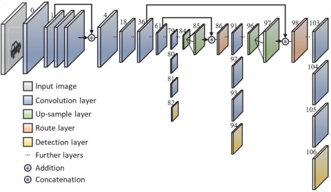
where, (σ) denotes the sigmoid function, (${{t}_{x}},~{{t}_{y}},~{{t}_{w}},~{{t}_{h}}$) represents the predicted values, and (${{c}_{x}},~{{c}_{y}}$) the coordinates of the top-left corner of the grid cell are the coordinates. (${{p}_{w}},~{{p}_{h}}$) refer to the dimensions of the anchor box. Figure 1 shows YLOLv3 architecture.

YOLOX is a single-stage object detection framework that is tailored for real-time applications. Important elements including residual modules, skip connections, and up-sampling procedures are incorporated into its structure. To provide prediction outputs, the model uses tiny 1×1 kernels and only convolutional layers. The detecting head has a kernel dimension of 1×1×255 and is based on the formula (B×(5+C))×1. Compared to previous iterations of the YOLO series, YOLOX offers better detection accuracy while operating at 30 frames per second (FPS) [28, 29]. The YOLOX model's detection pipeline consists of three main steps.

(1) Input Stage: To guarantee compatibility with the ensuing convolutional layers and preserve uniformity in spatial processing across the network, raw input images are resized to 608×608×3 (height×width×channels).

1a.png

1b.png

Figure 1. YOLOv3 architecture [30]

(2) Feature Extraction Stage: A deep convolutional network called the Darknet-53 backbone, which is intended to recognize hierarchical visual patterns, receives the scaled images. At 76×76, 38×38, and 19×19 spatial resolutions, this stage generates three unique feature maps that correspond to various receptive fields. From the original RGB channels to the 32, 64, 128, 256, 512, and finally 1024 filters, the feature maps are progressively deepened as the signal moves through the layers. These layers gradually pick up visual characteristics at low and high levels. Convolutional processing, up-sampling, down-sampling, and spatial-weighted feature fusion are all used in the ASFF method [31] to improve contextual representation once the acquired multi-scale features have been fused via an FPN.

(3) Prediction Stage: The detecting head uses the improved feature maps produced by the FPN and ASFF modules to make item predictions. Three anchor-based bounding boxes are produced by the model for every geographic grid cell. Multiple parameters obtained from the fused multi-scale features are encapsulated in each bounding box as Eq. (6):

$Number~of~Filters=\left( 5+C \right)\times B$    (6)

where, B indicates the quantity of anchor or boundary boxes that are used in the model, 5 represents the value of predictions for each bounding box (${{p}_{c}}$, ${{b}_{x}}$, ${{b}_{y}}$, ${{b}_{w}}$, ${{b}_{h}}$) and C represents the class probabilities.

3.4.1 Image augmentation

During pre-processing, data augmentation methods were used to improve the model's performance on dataset that were unbalanced. Specifically, image mix-up and label smoothing were utilized to improve the model generalization capacity and promote linear behaviour between training examples. Two examples are chosen at random for the image mix, X_i, Y_i and X_j, Y_j [32], and the creation of a new instance through linear interpolation, by the following Eqs. (7) and (8):

$\hat{x}=~\lambda {{x}_{i}}+\left( 1-\lambda  \right){{x}_{j}}$    (7)

$\hat{y}=~\lambda {{y}_{i}}+\left( 1-\lambda  \right){{y}_{i}}$    (8)

In these equations, X_i, Y_i and X_j, Y_j are two randomly selected samples from the training data, and $\lambda$ ∈ [0,1] is a value drawn from the Beta (β, β) distribution. This newly generated example ($\hat{x}$, $\hat{y}$) is then used in mix-up training. Moreover. Label smoothing regularizes the output distribution by softening the ground truth labels in the training data, thereby enhancing the model generalization ability. This technique introduces controlled noise to the actual class values, limiting the model capacity to overfitting and thus improving its overall classification accuracy [33].

3.4.2 Data augmentation methods

During testing and validation, this method was utilized to improve predictions for cases where the object in the image is too small. The images were resized using a randomly chosen interpolation technique from among the popular methods and then normalized [34].

3.4.3 ASFF

In the standard YOLOv3 model features through the FPN are fused in a top-down fashion to integrate deep and shallow feature information [29]; however, features at different scales remain interdependent and mutually constrained [35]. The ASFF process includes two key steps as follows [36]:

• Feature Resizing

In YOLOv3, for a given feature level l ∈{1,2,3} associated with a feature map ${{X}^{l}}$, the feature maps from all other levels ${{X}^{n}}$ where n ≠l, are spatially adjusted to conform to the resolution of (${{X}^{l}}$). This alignment is essential to enable effective multi-level feature aggregation. As YOLOv3 features across the three levels differ in resolution and channel numbers, up-sampling and down-sampling techniques are modified accordingly for each scale. followed by an interpolation to upscale the resolution.

• Adaptive Fusion

Concatenation along the channel dimension is performed once the tree-adjusted feature maps have been resized. After concatenation, the feature map is normalization through the soft-max activation function, generating weight vectors (α), (β), and (γ), which are then employed to combine the feature maps adaptively. The representation of the feature vector at spatial location ($i,~~j$) on the feature map that was moved from level n to level l is ($x_{ij}^{n\to l}$). At level l, the multi-scale feature aggregation can therefore be expressed as Eq. (9) [36, 37]:

$y_{ij}^{l}=~\alpha _{ij}^{l}.x_{ij}^{1\to l}~+~\beta _{ij}^{l}~.x_{ij}^{2\to l}~+~\gamma _{ij}^{l}.x_{ij}^{3\to l}$    (9)

where, ($y_{ij}^{l}$) indicate the output feature vector at ($i,~~j$) among channels, and weights ($\alpha _{ij}^{l}$), ($\beta _{ij}^{l}$), and ($\gamma _{ij}^{l}$) show how important feature mappings are spatially at three levels for level l, adaptively learnt, with shared across channels. Based on previous studies, the constraint ($\alpha _{ij}^{l}+~\beta _{ij}^{l}+~\gamma _{ij}^{l}~$= 1) is enforced, with values $\alpha _{ij}^{l}$, $\beta _{ij}^{l}$, $\gamma _{ij}^{l}$ ∈ [0,1] as Eq. (10) [36, 37]:

$\alpha _{ij}^{l}=~\frac{{{e}^{\lambda _{{{\alpha }_{ij}}}^{l}}}}{{{e}^{\lambda _{{{\alpha }_{ij}}}^{l}}}+{{e}^{\lambda _{{{\beta }_{ij}}}^{l}}}+~{{e}^{\lambda _{{{\gamma }_{ij}}}^{l}}}}$    (10)

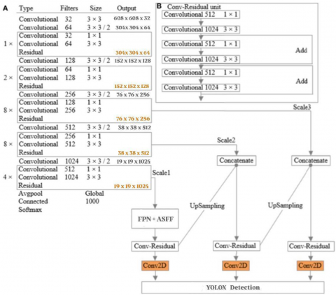
where, ($\alpha _{ij}^{l}$, $\beta _{ij}^{l}$) and ($\gamma _{ij}^{l}$) are determined using the softmax function, with the control parameters being ($\lambda _{{{\alpha }_{ij}}}^{l}$), ($\lambda _{{{\beta }_{ij}}}^{l}$), and ($\lambda _{{{\gamma }_{ij}}}^{l}$). Utilising 1×1 convolution layers, the weight scalar maps ($\lambda _{\alpha }^{l}$), ($\lambda _{\beta }^{l}$), and ($\lambda _{\gamma }^{l}$) are calculated from (${{x}^{1\to l}}$), (${{x}^{2\to l}}$), and (${{x}^{3\to l}}$) and are therefore learnable through standard backpropagation. This approach ensures each pixel in the fused feature map is a weighted average of corresponding pixels in the rescaled maps, uses adaptively learnt weights to improve detection accuracy and better integrate multi-level features. Table 1 and Figure 2 show Darknet-53 with ASFF in YOLOX architecture.

Table 1. YOLOX darknet-53 architecture

2.png

Figure 2. YOLOX architecture

5.1 Experiment and operating environment

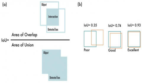
To assess the suggested YOLOX-based object identification model effectiveness in relation to AGV navigation, experiments were conducted using a well-structured and reproducible computational environment. The development and training processes were carried out within the Anaconda distribution, utilizing the PyCharm IDE and Python 3.11. The hardware configuration comprised a 13th Generation Intel® Core™ i7-1335U processor operating at 1.30 GHz, accompanied by 16 GB of system memory. The implementation relied on both TensorFlow and PyTorch frameworks to support efficient model construction and training flexibility. The training and testing dataset were generated through the combination of two benchmark datasets: Pascal VOC 2007 and Pascal VOC 2012. Specifically, the VOC 2012 dataset contributed 11,530 labeled images with 27,450 object annotations, while the VOC 2007 dataset provided 9,963 images containing 24,640 labeled objects. This combination resulted in a comprehensive dataset of 21,493 images and 52,090 object instances, representing a substantial and diverse collection of visual scenes. To ensure balanced learning and validation, 30% of the images were used for testing, while the remaining 70% were used for training. The large-scale dataset contributed significantly to improving model generalization and robustness across various object classes and environmental conditions. The training process utilized pre-trained Darknet53 weights as the initialization backbone. A total of 100 epochs were executed, comprising 8,275 iterations, with a 0.001 starting learning rate and a batch size of 16. To enhance convergence, an exponential decay strategy was applied every 20 epochs, reducing the learning rate by a factor of 0.9. 0.0005 weight decay regularization was also employed to prevent overfitting. Input images were resized dynamically between 320×320 and 608×608 pixels in order to reduce overfitting and enhance data variability, the model incorporates Mix-up and ASFF, supporting multi-scale object detection. Standard measures, namely Precision, Recall, and mAP, are used to evaluate performance. The IoU threshold was set to 0.8, ensuring that only predictions with substantial overlap with ground truth were accepted as true positives. An NMS threshold of 0.5 and a confidence score of 0.8 were applied.

4.png

Figure 4. Intersection over union [28]

5a.png

5a_2.png

5b.png

5b_-_fu_ben_.png

5c.png

5c_-_fu_ben_.png

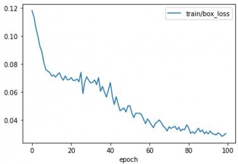
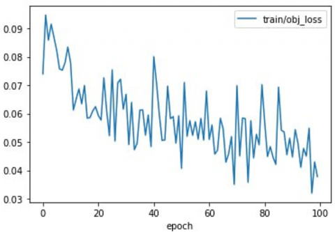
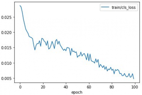
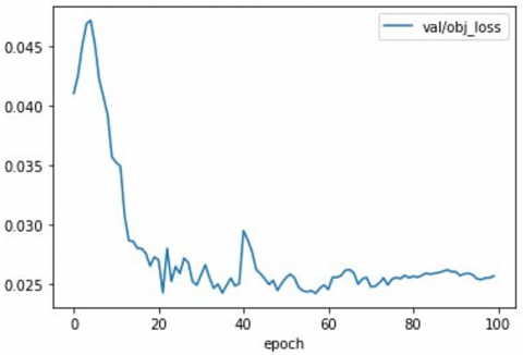
Figure 5. Results training and validation loss object, box, class vs. each epoch

As illustrated in Figure 4, IoU was used to measure detection accuracy by comparing predicted and ground truth boxes. The high IoU threshold, while reducing false positives, also presents a more rigorous standard, thereby balancing precision and recall in a meaningful manner. Figure 5 shows the loss value (object, box, class).

To examine robustness, the model was evaluated under different conditions, including variable lighting, partial occlusions, and dynamic backgrounds, to detect in real-world environments encountered by AGVs. Results indicate that the model retained high detection accuracy and decision reliability despite such environmental fluctuations, confirming its applicability to autonomous navigation in practical deployment scenarios.

5.2 Evaluation metrics

According to experiments, three metrics, Precision, Recall, and mAP, have been identified to assess the YOLO model's effectiveness in object detection.

Precision: the ratio of True Positive (TP) cases to all positive forecasts, quantifies how accurate positive predictions [34]. It is determined utilizing the Eq. (11):

$Precision=~\frac{TP}{TP~+~FP}$    (11)

Recall: measured as the percentage of actual positive predictions out of all potential positives, identifying missed positive predictions. It is measured utilizing Eq. (12) [34], where the number of TPs accurately predicted positive samples, while False Positive (FP) tracks incorrectly projected negative samples to be positive. Conversely, False Negatives (FN) tallies incorrectly projected positive samples to be negative. Due to the abundance of irrelevant background regions in images, True Negative (TN) is disregarded in evaluation, as these regions do not affect performance assessment. These metrics are crucial for evaluating classification model performance.

$Recall=~\frac{TP}{TP+FN}$    (12)

Mean Average Precision (mAP): known as the average precision (AP) across all detection categories, computed by averaging the AP values for each class. It provides a comprehensive assessment of model performance, calculated as the sum of AP values for all classes divided by the number of classes (N) in total [34], as Eq. (13):

$mAP=~\frac{1}{N}~\mathop{\sum }_{i=0}^{N}AP$    (13)

6a.png

6b.png

6c.png

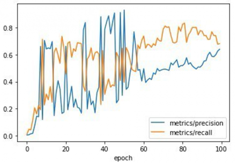
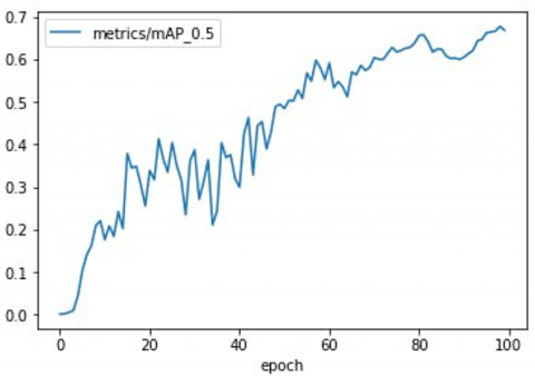
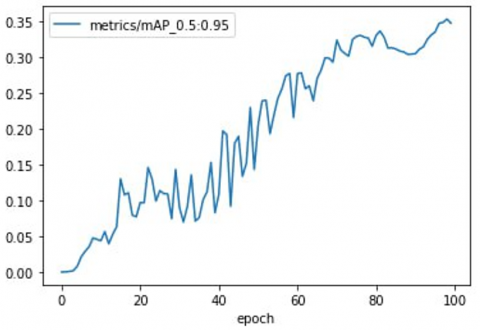
Figure 6. Evaluation metrics Precision, Recall, mAP@0.5, and mAP@0.5: 0.95

7.png

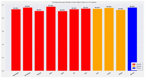
Figure 7. Average precision of dataset classes

The precision-recall curve's area under the curve is represented by this, where AP is computed over recall values at 0 and 1. mAP@0.5:0.95 averages mAP across IoU thresholds from 0.5 to 0.95, whereas mAP@0.5 denotes mAP at an IoU threshold of 0.5 itself. mAP also varies with confidence thresholds. Figure 6 shows the analysis of Recall, Precision, mAP@0.5:0.95 and mAP@0.5 for YOLOv3 on the Pascal VOC validation dataset. The results demonstrate significant improvements in performance metrics. Precision increased from 0.0039 at epoch 1 to 0.6405 at epoch 100, while recall rose from 0.0088 to 0.6815. Both mAP@0.5 and mAP@0.5:0.95 improved from 0.0002 to 0.3472 and from 0.0010 to 0.6685, respectively. The AP values, which indicate precision at various recall levels, showed high accuracy across all classes, as shown in Figure 7.

This study presents a real-time control system for Forklift AGVs that combines deep learning-based object detection with adaptive motion handling. The system integrates an improved YOLOX model supported by ASFF, where spatial weights (α, β, γ) contribute to better feature representation across different scales. Experimental results showed that the system can accurately detect small, distant, overlapping, and partially visible objects under various lighting conditions, achieving a detection precision exceeding 97%. The Forklift AGV demonstrated stable navigation across three obstacle scenarios—clear paths, medium-range objects, and close obstacles—with consistent responses such as stopping or re-routing. The system maintained reliable real-time performance even on resource-constrained hardware, confirming its applicability in industrial environments. However, the current implementation is limited to reactive navigation without predefined path planning within a fixed indoor industrial layout. Future work will focus on extending the system to support multi-AGV coordination and integrating additional sensing capabilities to enable site-level path planning.