Ibrahim M. Ramadan*![]() | Alaa A. Ahmed
| Alaa A. Ahmed![]() | Mahmoud M. Salim
| Mahmoud M. Salim![]()
© 2024 The authors. This article is published by IIETA and is licensed under the CC BY 4.0 license (http://creativecommons.org/licenses/by/4.0/).
OPEN ACCESS
This study aims to assess the probability of unsafe operations on horizontal curves resulting from speed variation, employing both statistical analysis and machine learning (ML) techniques. The statistical analysis was conducted using Minitab software to assess the probability of non-compliance through the Monte-Carlo simulation method. Additionally, the research applied three ML classification models—a novel optimized version of the Random Forest (RF) classifier, Naive Bayes (NB), and Extreme Gradient Boosting (XGBoost). Nine curves with radii ranging from 700m to 2000m were selected from two rural roads in Egypt for the study. The evaluation of non-compliance probability on each curve involved contrasting the supply (design speed, a fixed value) with the demand (actual speed, characterized by actual speed distributions). Findings revealed that using the 85th percentile speed in the analysis, the probability of non-compliance during off-peak hours exceeded 50% for all curves except two, where it reached 100%. This indicates that approximately 100% of vehicles engage in unsafe operations during off-peak hours on these specific curves. Accuracy results of the ML classifiers showed that the proposed RF classifier performed exceptionally well with a perfect score of 1.0, followed by XGB and NB classifiers for all curves. A comparative analysis between the results of statistical analysis and ML in estimating curve safety suggests that ML outperforms statistical analysis, demonstrating its potential as a more reliable tool for assessing road safety on horizontal curves.
reliability, statistical analysis, machine learning, horizontal curves safety, speed variation
Traditionally, road design relies on a set speed value specified in manuals. However, it's crucial to acknowledge the non-uniform nature of vehicle speeds, which vary among different vehicles and over time, occasionally exceeding the designated design speed. Vehicles surpassing the intended speed limit may operate unsafely on the road. Therefore, the key questions are: how many vehicles exceed the speed limit, and what percentage of operations are unsafe? To address this issue, it is essential to examine the percentage of vehicles engaging in unsafe operations. This analysis should be conducted, determined, and integrated into the design process. Consequently, numerous studies have aimed to incorporate a variable speed value, as opposed to a fixed one, in the design and analysis of road safety. This approach involves considering speed variations and evaluating the safety of road elements to assign specific safety levels. While general road safety encompasses a broad range of factors affecting all types of roadways, the specific focus on horizontal curve safety zeroes in on the unique challenges these curves present, such as increased risk of skidding and loss of control, which are exacerbated by variations in vehicle speed.
A notable case study illustrating the consequences of not accommodating variable speeds in road design is the frequent accidents on the curved sections of the Pacific Coast Highway (PCH) in California. This scenic route is known for its sharp, winding curves and varying speed limits, which can catch drivers off guard, particularly those unfamiliar with the road. In several high-profile incidents, such as the fatal crash involving actor Paul Walker in 2013, it was evident that speed variations combined with the road's curvature contributed significantly to the loss of control. These incidents highlight the critical need for road designs that better accommodate speed variations through improved signage, road surface treatments, and geometric adjustments, thereby enhancing driver awareness and safety on such challenging segments.
The research gap in horizontal curve safety due to speed variation lies in the limited understanding of how different speed variations interact with road geometry and driver behavior to influence accident risk.
In this context, examining a road's maximum allowable safe speed, typically a fixed parameter requires a comparison with the inherently variable nature of the demand for vehicle speed. The result of this analysis clarifies the likelihood of noncompliance within the road infrastructure. This study specifically delves into the probability of vehicles deviating from compliance due to speed variations on horizontal curves. Two techniques are employed in this research: the first relies on statistical analysis, determining the normal distribution of speed (representing demand) as a focal point, alongside estimating the actual design speed of the horizontal curve (representing supply). The probability of noncompliance (Pnc) will be systematically calculated by comparing these two elements- demand and supply [1].
Research on horizontal curve safety due to speed variation is essential and innovative, as it involves a key aspect of road safety. The speed variations on horizontal curves can result from various factors, including road conditions, driver behavior, and vehicle performance. Understanding the impact of these variations on safety is essential for developing more effective road design and traffic management strategies. The research aims to reduce accidents and enhance overall traffic safety by focusing on this area. It offers new insights that can inform policies and engineering solutions designed to mitigate the risks associated with speed variations on curves [2].
This research examines road safety at horizontal curves influenced by speed variation using both statistical analysis and machine learning (ML) techniques. It introduces the safety study methodology for each approach and compares their accuracy, finally recommending the more effective procedure. The recommendations from this research should be incorporated into the design manuals of each country, emphasizing the need to consider speed variations in the design process instead of relying on fixed speeds. In essence, ML exceeds conventional statistical models due to its capacity to handle complex, nonlinear relationships in data, process large and diverse datasets, capture complicated interactions among various factors, adapt and optimize performance iteratively, and provide more accurate assessments of non-compliance and crash risk, and finally enhancing road safety efforts [3].
Road safety studies involve a broad examination of various elements essential for understanding and improving traffic safety. These studies investigate the complex interactions among affecting factors such as road geometry, traffic characteristics, vehicle features, and environmental conditions. Geometric elements include road design, signage, and intersection layout. Traffic flow patterns, driver behavior, and the effects of weather conditions and visibility are integral components of road safety studies. Additionally, analyses of accident data, injury severity, and the effectiveness of safety interventions provide a fundamental insight. The incorporation of emerging technologies, such as intelligent transportation systems and advanced data analytics, enhances these studies, enabling a more nuanced understanding of the dynamic factors influencing traffic safety. The combination of these various elements in traffic safety studies forms a foundation for decision makers, engineering interventions, and educational campaigns aimed at the enhancement of traffic safety [4, 5].
Variations in vehicle speeds on horizontal curves introduce a dynamic element to the traffic environment, significantly affecting the likelihood and severity of accidents. Speed fluctuations can lead to reduced reaction times, increased braking distances, and compromised vehicle control, all of which contribute to a higher risk of collisions. Excessive speeds, particularly when they deviate from the average or posted limits, exacerbate the severity of accidents. Conversely, quick reductions in speed or significant speed differentials between vehicles can result in a high risk of traffic accidents. Investigating the correlation between speed variation and traffic accidents is essential for developing effective measures to mitigate risks and enhance overall traffic safety [6, 7].
Examining the relationship between driver behavior and speed on horizontal curves is an essential aspect of traffic safety research. Drivers' reactions to horizontal curves significantly influence the determination of an appropriate and safe speed for navigating these curves. Factors such as perception time, mental workload, and individual driving experience contribute to variations in driver behavior. Understanding how drivers adapt to the geometry of horizontal curves and weigh their own comfort and safety margins is essential for optimizing road design and reducing the risk of accidents. Technical investigations into this relationship explore the cognitive processes involved in speed perception, decision-making, and the execution of appropriate speed adjustments, providing valuable insights for developing effective countermeasures aimed at enhancing the safety of horizontal curves on roadways [5, 8, 9].
Alhomaidat [1] developed a model to explore the correlation between accident rates and speed on arterial and freeway roads. They found that the average 85th percentile speed of vehicles exiting the freeway is 70 mph. This speed is higher than that on the arterial streets. This affects the safety of that road. Additionally, their study revealed that an increase in the speed limit could lead to a 13.9% rise in accident rates, particularly on arterial streets [9]. In a study by Alnawmasi and Mannering [10], the impact of altering speed limits on road safety features was also investigated. The researchers concluded that changes in speed limits do not significantly affect the frequency of crashes but do have a modest impact on the severity of injury accidents [10].
Faiz et al. [11] conducted a study on speed variation on two-way two-lane rural roads in Malaysia, focusing on light vehicles during nighttime and morning operations. The results highlighted a relationship between the curve radius and the speed of each vehicle type. In a study by Gaber et al. [12], various factors influencing road safety were examined, including pavement conditions, speed, traffic volume, road entrance characteristics, traffic sign conditions, and road width. The research indicated a probable 5.26% reduction in the accident rate when using a lane width of 3.5m. Furthermore, a reduction in the speed limit to 75 km per hour could lead to a 7.38% decrease in the accident rate. Additionally, maintaining good pavement conditions was associated with a substantial 17.9% reduction in the accident rate [12].
The influence of traffic composition on traffic accidents creates a complex and multifaceted area of research. The makeup of traffic, surrounding of vehicle types, sizes, and driving behaviors, significantly outlines the risk opportunity on roadways. Understanding how traffic mix interacts is essential for understanding patterns of accidents. For example, the existence of vehicles with different speeds, management capabilities, and braking distances presents complexities that can increase the likelihood and severity of traffic accident. Moreover, variations in driver experience, vehicle size, and road user categories contribute to the complicated dynamics of traffic safety. Studies examining the impact of traffic composition on accidents often employ advanced modeling techniques, statistical analyses, and observational data to discern patterns and fundamental relationships. Conclusions derived from such studies are important for planning targeted interventions and traffic management strategies aimed at reducing accident rates and enhancing overall road safety in diverse traffic environments [13, 14].
The impact of geometrical characteristics of roads on traffic safety is also an important area in safety research. Features like road alignment, lane width, intersection design, and road curvature greatly influence vehicular movement and safety. Well-designed geometrical features contribute to smoother traffic flow, reduce conflict points, and enhance visibility, and finally mitigate the risk of traffic accidents. Conversely, inadequately configured geometrical characteristics can increase the likelihood of collisions, especially at intersections or on curves where visibility is compromised. Advanced research in this field utilizes techniques such as geometric design consistency analysis and computer simulations to assess the relationship between specific geometric features and safety outcomes. These studies provide valuable insights for traffic engineers, aiding in the implementation of road designs that prioritize safety and contribute to an overall enhancement of road safety [4, 15].
Goswami [16] employed intelligent transportation systems to estimate road accident rates, utilizing geographical information systems (GIS) as a key tool for determining road safety factors. Similarly, Jimee et al. [17] utilized GIS for accident analysis in Nepal, categorizing accidents based on vehicle type, driver behavior, and other relevant factors. The study revealed that a significant factor contributing to accidents is the adherence to design manual limits, particularly evident in the minimum lane width and sight distance and their correlation with the design speed [17].
Exploring the correlation between non-compliance probability and crash risk on high-speed curves is a critical aspect of understanding and improving road safety. Numerous researches suggest valuable insights into this relationship, drawing attention to factors that contribute to the vulnerability of drivers and vehicles when crossing curves at high speeds. These documents often incorporate data from comprehensive studies, collision analyses, and traffic safety research. By scrutinizing the probability of non-compliance with recommended speed limits on curves, researchers can distinguish patterns and trends associated with an increased likelihood of crashes. This information is vital for developing effective countermeasures and safety measures to mitigate the risks linked to high-speed curves. Understanding the nuanced relationship between non-compliance and crash risk not only informs engineering standards and road design but also guides policy and enforcement strategies aimed at promoting safer driving behavior on challenging road geometries [18, 19].
The preceding discussion highlights various research endeavors focused on exploring the connection between speed and accident rates. Nonetheless, a limited number of studies have approached speed variation from a statistical standpoint. Consequently, this research aims to assess the likelihood of non-compliance for a specified curve and speed profile utilizing two distinct techniques: statistical analysis and ML.
The purpose of this section is to elucidate the necessary data and the methodology employed for its collection. The gathered data encompass both geometrical and traffic characteristics of nine horizontal curves situated on regional highways in Egypt. These highways comprise the ring road (consisting of five curves), Cairo Alex desert road (with two curves), and Cairo Elsokhna Road (featuring two curves). The nine curves are chosen randomly on the above-mentioned roads.
The first step in traffic data collection is determining the off-peak hour. Traffic volume on each road was manually counted for 12 hours, from 7 am to 7 pm. A fluctuation chart was created for each road. The results indicated that the off-peak hour for the Cairo-Alex Desert Road is from 11 am to 12 pm, and for the Ring Road, it is from 1 pm to 2 pm. Traffic data for each curve was acquired through a video recording process conducted during the above-mentioned off-peak hours to capture maximum speed values. A video camera was positioned on each curve, providing comprehensive coverage of the entire curve length. The collected traffic data encompassed information on traffic volumes and speeds.
The geometrical characteristics of the curves were sourced from the design drawings of these curves and subsequently validated using Google Earth. A summary of the collected geometrical characteristics of the curves is presented in Table 1.
Table 1. Data set statistical summary of the studied horizontal curves
|
No. |
Lanes |
Lane Width (m) |
Shoulder Width (m) |
Radius (m) |
Superelevation (%) |
Deflection Angle Δ0 |
Curve Lngth L (m) |
Middle Ordinate-M (m) |
|
1 |
8 |
3.65 |
2.5 |
700 |
6 |
105 |
1283 |
4.325 |
|
2 |
8 |
3.65 |
2.5 |
800 |
5 |
72 |
1005 |
4.325 |
|
3 |
8 |
3.65 |
2.5 |
1000 |
4 |
34 |
602 |
4.325 |
|
4 |
8 |
3.65 |
2.5 |
1250 |
3.5 |
57 |
1238 |
4.325 |
|
5 |
8 |
3.65 |
2.5 |
2000 |
2 |
60 |
2068 |
4.325 |
|
6 |
6 |
3.75 |
2.5 |
1000 |
5.6 |
54 |
930 |
9.375 |
|
7 |
6 |
3.75 |
2.5 |
750 |
6 |
77 |
1000 |
9.375 |
|
8 |
6 |
3.75 |
2.5 |
900 |
6 |
48 |
750 |
11.30* |
|
9 |
6 |
3.75 |
2.5 |
1350 |
4.5 |
55 |
1300 |
7.50* |
Note: *According to the minimum middle ordinate for AASHTO and Egyptian code design
Table 2. Data summary of the speed of the studied horizontal curves
|
Curve No. |
85thPercentile Speed V85 |
Standard Deviation SD85 |
Average Speed Vmean |
Standard Deviation (SDmean) |
Mean Vmax - Operating |
|
1 |
95.61 |
3.4187 |
87.79 |
7.527 |
105.13 |
|
2 |
104.6 |
1.6651 |
93.27 |
8.9553 |
106.62 |
|
3 |
107.25 |
4.5738 |
96.24 |
8.959 |
111.16 |
|
4 |
106.41 |
4.2427 |
97.69 |
5.2498 |
108.61 |
|
5 |
108.35 |
1.4542 |
101.44 |
5.5293 |
107.30 |
|
6 |
129.95 |
2.3319 |
118.66 |
7.4007 |
128.64 |
|
7 |
120.54 |
3.2058 |
113.74 |
4.4706 |
128.29 |
|
8 |
122.74 |
4.4216 |
113.39 |
5.5638 |
125.60 |
|
9 |
128.03 |
3.1314 |
120.98 |
5.6815 |
126.23 |
The velocity measurement in this study involved assessing the time taken to traverse the entire length of the curve. In Table 2, the research team presents data including the average eighty-fifth percentile speed (V85) with its standard deviation (SD85), mean speed (Vmean) with its standard deviation (SDmean), and maximum speed observed on each curve (Vmax). Each curve's sample size comprised 150 vehicles. Speed analysis, facilitated by SPSS software, followed a structured approach, which included organizing speed data into sets based on 1-minute intervals recorded by the Video Camera. Subsequently, the 85th percentile speed for each group was computed using SPSS software. The study then established the average of the 85th percentile speeds for each curve, with the standard deviation calculated to account for variance among the averages of the groups for each curve.
Tables 1 and 2 clearly demonstrate that the curve radius alone does not exclusively dictate the 85th percentile speed. Even when the radii are nearly identical, there are observed differences in speeds. It is noteworthy that the designated speed for the ring road is 100 km per hour (curves 1 to 5), while the design speed for the Cairo Alex desert road and Cairo Elsokhna desert road is 120 km per hour (curves 6 to 9).
4.1 Probability distributions for the random input parameters
In this research, the Minitab software was employed by the research team to assess the probability of non-compliance through the Mont-Carlo simulation method. Each curve is characterized by a singular deterministic value of design speed, along with operational speed attributes such as mean and standard deviation. The estimation of the probability of non-compliance involved utilizing both the design speed and the 85th percentile speed of vehicles surpassing the designated speed on the respective curve
Using the 85th percentile speed is crucial in estimating horizontal curve safety because it more accurately reflects the behavior of the majority of drivers compared to the average speed or any other measure. The 85th percentile speed represents the speed at or below which 85% of vehicles are traveling, thereby capturing the speed that most drivers consider safe under current road conditions. This approach helps in designing curves that accommodate natural driving patterns, reducing the risk of accidents caused by discrepancies between actual driving speeds and design speeds. By aligning road design with the 85th percentile speed, engineers can create safer, more efficient roads that better account for real-world driving behavior and variability in speed, leading to improved overall safety on horizontal curves.
4.2 Calculation of non-compliance probability
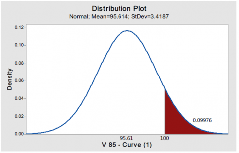
Utilizing the Minitab software, the speed distribution has been graphed based on the 85th percentile speed for each curve, as elaborated in the preceding section. The design speed is then plotted against the speed distribution for each curve, and the probability of non-compliance is calculated. Figure 1 illustrates the probability of non-compliance when employing the 85th percentile speed distribution. It is evident from Figure 1 that approximately 10% of operations exhibit unsafe conditions when utilizing the 85th percentile speed.
It is noteworthy that the probability of non-compliance arises when the actual vehicle speed surpasses the designated design speed. Therefore, the probability of non-compliance is estimated as the difference between the design speed and the mean of 85th percentile speed. That means the probability of non-compliance occurs when the actual mean speed is greater than the design speed.
Figure 1. The probability of non-compliance (Pnc) of V design for curve no.1 by V85 distribution
4.3 Results of non-compliance probability, reliability, and discussion
The outcomes of the probability of non-compliance estimation for speed variations across the nine curves are presented in Table 3. It is evident from the table that the probability of non-compliance reaches 100% for curves 4 and 5, and exceeds 90% for curves 2, 3, 4, and 9. This implies that all vehicles operate under unsafe conditions during off-peak hours.
The results above indicate a high probability of non-compliance for most examined curves. This outcome appears logical and compatible with the literature due to several factors, including low traffic volumes during this time period, the absence of speed-detecting devices in these areas, the favorable conditions of the roads, or drivers perceiving the speed limit as incredible. A credible speed limit is one that drivers find logical and appropriate, considering the road's characteristics and immediate surroundings. This includes factors such as road type, layout, surface, curvature, traffic density, weather conditions, and traffic mix. Consistency and continuity in road design are essential, ensuring that each road scene matches a speed limit accepted by most drivers [2, 20]. The problem of noncompliance is a major cause of motor vehicle collisions and significantly contributes to their severity and catastrophic outcomes. Reducing
Therefore, work should be done to force drivers to follow the speed limit. Driving speed is a prudent strategy to enhance road safety.
Table 3. Summary of reliability results of speed according to V85 of horizontal curves
|
Curve No. |
Radius (m) |
V Design |
V85 |
SD |
Pnc |
R |
|
1 |
700 |
100 |
95.61 |
3.4187 |
9.97 |
90.03 |
|
2 |
800 |
100 |
104.6 |
1.6651 |
99.71 |
0.29 |
|
3 |
1000 |
100 |
107.25 |
4.5738 |
94.35 |
5.65 |
|
4 |
1250 |
100 |
106.41 |
4.2427 |
93.46 |
6.54 |
|
5 |
2000 |
100 |
108.35 |
1.4542 |
100 |
0 |
|
6 |
1000 |
120 |
129.95 |
2.3319 |
100 |
0 |
|
7 |
750 |
120 |
120.54 |
3.2058 |
56.7 |
43.3 |
|
8 |
900 |
120 |
122.74 |
4.4216 |
73.23 |
26.77 |
|
9 |
1350 |
120 |
128.03 |
3.1314 |
99.48 |
0.52 |
The authors applied three classification models in this research NB, XGBoost, and RF, hereafter, an explanation of each classifier is introduced.
5.1 Naive Bayes (NB)
The NB algorithm uses Bayes' theorem as its foundation for probabilistic categorization [21-23]. It streamlines probability computation by assuming that, given the class label, the features are conditionally independent. NB is great for situations when there isn't a lot of training data because it can quickly manage several features in our classification problem. Using the observed feature values, the classifier can help to determine the likelihood of a vehicle's safety.
5.2 Extreme Gradient Boosting (XGBoost)
Extreme Gradient Boosting, or XGBoost for short, is a scalable and very effective ensemble learning technique [24]. It generates weak learners (usually decision trees) in a sequential fashion, with each one fixing the mistakes of the one before it. The prediction accuracy is improved by XGBoost with the use of gradient boosting techniques and a regularization term. Its superior predictive power makes it an excellent choice for complicated datasets.
5.3 Random Forest (RF)
An additional ensemble learning approach, RF builds a large number of decision trees during training and then produces the class mode as a classification output. It selects subsets of features and occurrences at random, which introduces randomness into the tree-building process. A more resilient model is the result of the increased diversity and decreased overfitting caused by this randomness [11, 25].
The authors applied the following metrics to check the accuracy of the applied classifier models.
6.1 Confusion matrix
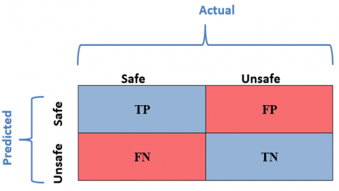
By offering a comprehensive breakdown of actual and expected class memberships, the confusion matrix is an essential tool for assessing the efficiency of categorization algorithms [2]. True positives (TP), false positives (FP), true negatives (TN), and false negatives (FN) are the four basic metrics represented by the square matrix. Whereas FP denotes situations where the model incorrectly classified a safe vehicle as unsafe, TP denotes instances where the model accurately predicted the safety of a vehicle in relation to our road curve classification job. When the model successfully identified a vehicle as unsafe, it will display TN, and when it wrongly classed a safe vehicle as unsafe, it will display FN. Here is the structure of the matrix as shown in Figure 2.
Figure 2. The structure of the confusion matrix
Elements that are off the diagonal (FP and FN) represent misclassifications. However, elements on the diagonal (TP and TN) show accurate forecasts. To better understand the classifier's capabilities and limitations while dealing with the complexities of road curve safety, this detailed breakdown enables the computation of essential assessment metrics including recall, accuracy, precision, and F1-score [2, 26].
6.2 Area under the curve (AUC)
It is worthy to mention that, the Area Under the Receiver Operating Characteristic (ROC) Curve (AUC) provides a brief assessment of a model's capacity to distinguish between positive and negative cases. As one moves from one decision threshold to another, the ROC curve shows the relative importance of sensitivity (the rate of true positives) and specificity (1-specificity) in relation to the true positive rate. A higher area under the curve (AUC), which ranges from 0 to 1, suggests stronger discriminating performance. An improved area under the curve (AUC) indicates that the classifier successfully differentiates between safe and unsafe vehicles using the given features, offering a thorough evaluation of its prediction power in the context of road curve classification.
6.3 Accuracy
The accuracy of a classifier is defined as the percentage of correctly predicted instances relative to the total number of instances, which is represented by Eq. (1):
Accuracy $=\frac{T P+T N}{T P+T N+F P+F N}$ (1)
6.4 Precision
Precision is calculated as the ratio of true positive predictions to the total number of predicted positives, measuring the accuracy of positive predictions given by Eq. (2):
Precision $=\frac{T P}{T P+F P}$ (2)
6.5 Recall (Sensitivity or true positive rate)
As a measure of the classifier's performance, recall is calculated as the percentage of positive predictions that turned out to be true divided by the total number of positive occurrences as Eq. (3):
Recall $=\frac{T P}{T P+F N}$ (3)
6.6 F1-score
The harmonic mean of recall and precision is the F1-score. The measure strikes a good balance between recall and precision represented by Eq. (4):
F1-score $=\frac{2 \times \text { Precision } \times \text { Recall }}{\text { Precision }+ \text { Recall }}$ (4)
Taken as a whole, these metrics provide a thorough evaluation of the classifiers' performance on the road curve categorization job.
In this paper, we propose an optimized version of the RF classifier to distinguish between the safe/unsafe vehicles regarding a certain road curve. Besides, the proposed RF model is compared against the NB and XGB classifiers showing its consistency and perfect results with accuracy of 100%.
The three techniques mentioned above were applied to analyze three curves that have been picked up from the aforementioned highways i.e., the ring road, Cairo Alex desert road, and Cairo Elsokhna Road to be investigated in order. The software used includes PyCaret version 3.3.2, an open-source, low-code machine learning library with Python v3.10.12. Subsequently, the following section delves into the discussion of this application.
7.1 The ring road curve
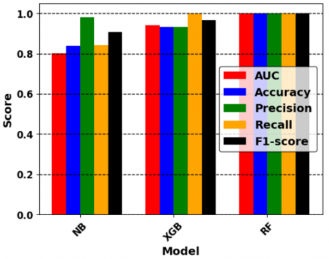
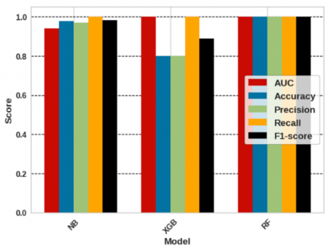
Figure 3 illustrates a bar chart that shows the simulated results for three classifiers i.e., NB, XGB, and proposed RF for the ring road curve. It compares models’ performance across various evaluation metrics such as AUC, Accuracy, Precision, Recall, and F1-score. It can be seen how each classifier is doing in different areas thanks to the color-coded representation.
The AUC values of all the classifiers are very high; RF achieved a flawless score of 1.0. Results for accuracy demonstrate that the RF classifier performs admirably with a perfect score of 1.0 followed by the XGB and then the NB classifier. Again, the RF-optimized classifier shows an outstanding precision performance of 1.0, whereas the NB comes after and the XGB comes last. The classifiers' capacity to catch all positive cases is highlighted by the Recall metric, which displays faultless performance by XGB and RF. The F1-score bar gives a remarkable result in the case of the proposed RF classifier that equals 1.0 in contrast to the others. In our simulated road curve classification situation, the optimized RF classifier performs better than the XGB and NB classifiers according to the given dataset with a perfect performance.
Figure 3. Comparative performance of NB, XGB, and proposed RF classifiers for ring road curve
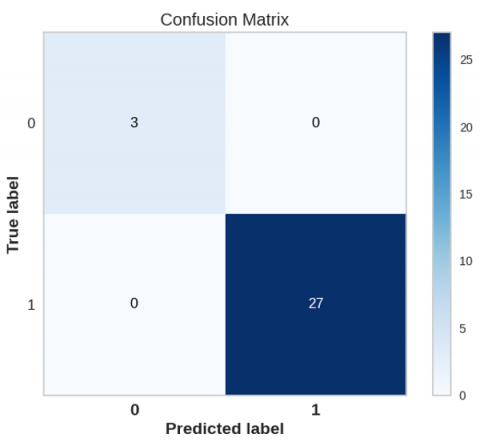
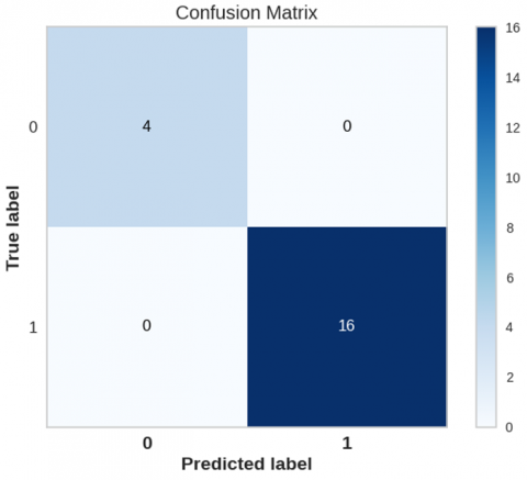
Figure 4. Proposed RF model confusion matrix for ring road curve
One of the main tools for evaluating classification problems is the confusion matrix, which shows how well the predicted classes perform. As shown in Figure 4, we have discovered that the RF model achieves the best classification accuracy when differentiating between the safe/unsafe events following a comprehensive examination. The findings show that every dataset used successfully predicts the labels of safe "1" with a perfect score. Similarly, unsafe "0"'s label prediction is 100% accurate.
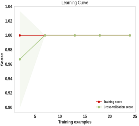
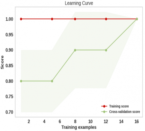
We display the learning curves of our RF best model for both the training and cross-validation runs in Figure 5 to prove its effectiveness. According to the figure, the RF model outperforms all others, with a training accuracy of 100% and a cross-validation accuracy of 100% as well. In particular, there is no room for improvement when the no fluctuating curve is present. In addition, there is a strong correspondence between the training and cross-validation curves, which shows that the model is effective.
Figure 5. Learning curves for the RF model for ring road curve
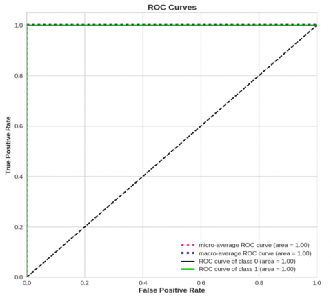
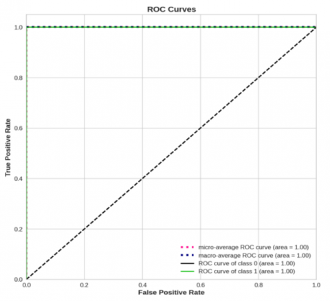
Figure 6. The ROC curves of the proposed RF model for ring road curve
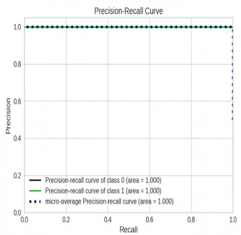
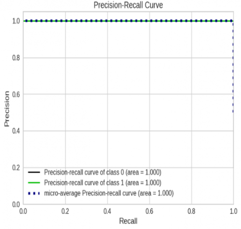
Figure 7. The precision-recall results of the proposed RF model for ring road curve
One way to visualize the correlation between the projected class's TP and FP rates is using the ROC curve. In terms of classification accuracy, our comprehensive investigation shows that the RF model regularly performs better than the others. The ROC curves that were generated by classifying safe and unsafe events using the superior RF model are shown in Figure 6. Successful classification rates of 100% for safe class "1" as well as unsafe class "0" are recorded.
The link between recall and precision for the most accurate strategy in terms of classification accuracy is shown in Figure 7. After exhausting all other available ML models, we exclusively show the precision-recall result based on the RF (best model). The RF model can differentiate between safe and unsafe events with a 100% accuracy rate.
7.2 Cairo Alex desert curve
Considering the results of the Cairo Alex desert curve, the XGB and optimized RF classifiers have AUC values of a perfect score of 1.0 in contrast to the NB classifier with less value shown in Figure 8. According to the accuracy results, the RF classifier is the best with a score of 1.0, followed by the NB classifier with a slight difference, while the XGB classifier comes after them at 0.8. The RF-optimized classifier once again outperforms the NB and XGB with a precision performance of 1.0. The recall statistic showcases the classifiers' ability to catch all positive examples with a perfect performance of 1.0. In contrast to the others, the suggested RF classifier achieves an impressive F1-score bar value of 1.0, while that of the NB and XGB classifiers are 0.984 and 0.889, respectively. In a nutshell, the modified RF classifier outperforms the XGB and NB classifiers in our simulated road curve classification scenario with perfect results proven by all the evaluation metrics.
After conducting a thorough investigation, it is found that the RF model yields the highest classification accuracy when distinguishing between safe and unsafe events as illustrated by the confusion matrix in Figure 9. Results demonstrate that all datasets accurately forecast the labels of safe "1" with a flawless score. Likewise, the label prediction for unsafe "0" is spot on with 100% accuracy.
Figure 8. The evaluation metric for different classifiers for Cairo Alex desert curve
Figure 9. Confusion matrix of the proposed RF model for Cairo Alex desert curve
Figure 10. RF proposed model's learning curves for Cairo Alex desert curve
Figure 11. ROC curves of the proposed RF model for Cairo Alex desert curve
Figure 12. RF model’s precision and recall for Cairo Alex desert curve
As evidence of its efficacy, we show in Figure 10 the learning curves of our RF best model during the training and cross-validation cycles. The RF model is clearly the best option, since it achieves a perfect score in both the training and cross-validation phases, as shown in the figure. Specifically, in the presence of the non-fluctuating curve, there is no possibility for progress. The model is also effective since the training and cross-validation curves are very congruent with one another.
As aforementioned, the ROC curve is a useful tool for visualizing the relationship between the predicted class's TP and FP rates. According to our extensive research, the RF model consistently outperforms the competitors in terms of classification accuracy. Figure 11 shows the ROC curves that were produced by categorizing events as safe or unsafe using the better RF model. Both the safe class "1" and the unsafe class "0" have 100% success rates in categorization.
Figure 12 shows the correlation between recall and precision for the best classification accuracy technique. Once we've tried every other ML model, we'll only display the accuracy-recall metric for the RF model i.e., best model. The RF model has a perfect track record of accurately identifying safe and unsafe occurrences.
7.3 Cairo Elsokhna curve
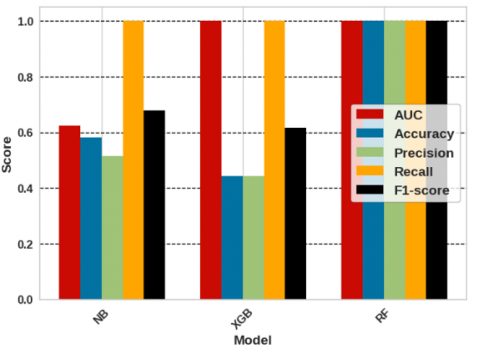
As illustrated by Figure 13, the Cairo Elsokhna curve, the optimized RF and XGB classifiers outperform the NB classifier in terms of AUC, which is about 0.625 in the case of the NB model. By a wide margin, the XGB classifier comes in at 0.444, while the NB classifier takes last place with a score of 0.581, as shown by the accuracy results. With a precision performance of 1.0, the RF optimized classifier once again surpasses the NB and XGB. Fortunately, all the classifiers' capacity to detect all positive examples with a flawless performance of 1.0 is demonstrated by the recall statistic. While the NB and XGB classifiers get F1-score bar values of 0.679 and 0.616, respectively, the proposed RF classifier stands out with an amazing 1.0. To summarize, in our simulated road curve classification situation, the updated RF classifier achieves better results than the XGB and NB classifiers, as evidenced by all assessment criteria.
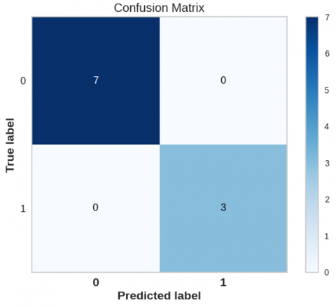
As shown in Figure 14's confusion matrix, an exhaustive analysis reveals that, when it comes to differentiating between safe and unsafe occurrences, the RF model produces the highest classification accuracy. The results show that every dataset performed perfectly when it came to predicting the labels of safe "1". Similarly, the unsafe "0" label prediction is also 100% accurate.
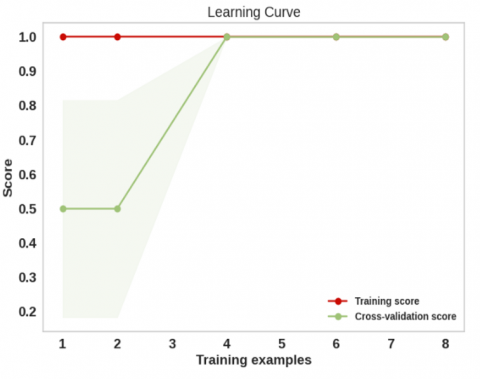
Our RF best model's learning curves across training and cross-validation cycles are displayed in Figure 15, demonstrating its effectiveness. Based on its flawless performance in both the training and cross-validation stages, the RF model stands out as the top choice, as illustrated in the figure. In particular, advancement is impossible when the non-fluctuating curve is present. Due to the high degree of congruence between the training and cross-validation curves, the model is likewise effective.
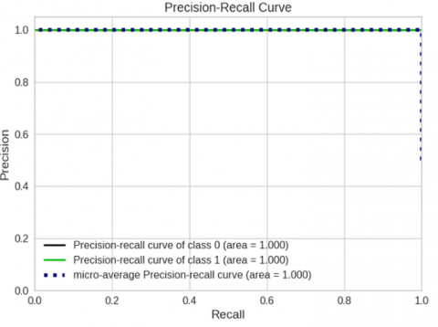
The best classification accuracy technique's recall and precision correlation is shown in Figure 16. After all the ML models have been exhausted, we will simply show the accuracy-recall metric for the best RF model. In terms of reliably determining which events are safe and which are not, the RF model has never failed.
Figure 13. The evaluation metric for different classifiers of Cairo Elsokhna curve
Figure 14. Confusion matrix of the proposed RF algorithm for Cairo Elsokhna curve
Figure 15. The learning curves of the RF proposed algorithm for Cairo Elsokhna curve
Figure 16. RF model’s precision and recall for Cairo Elsokhna curve
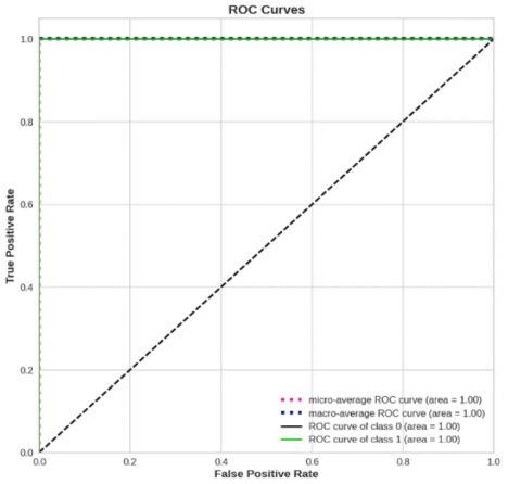
Figure 17. ROC curves of the proposed RF model for Cairo Elsokhna curve
In order to see how the TP and FP rates of the projected class relate to one another, the ROC curve can be a helpful tool. Our findings indicate that when compared to its rivals, the RF model routinely achieves superior classification accuracy. The improved RF model was used to classify events as safe or unsafe, and the resulting ROC curves are displayed in Figure 17. Classification success rates are 100% for both the safe "1" and unsafe "0" classes.
7.4 Train-test split and tuned hyperparameters
Table 4 presents the train-test split as well as the tuned hyperparameters (HPs) for different ML models applied to various curves. HPs play an essential role in determining the performance and behavior of ML algorithms. Through systematic changes, optimal values are selected to enhance model efficiency and generalization ability across different scenarios.
The potential of ML models in predicting non-compliance and assessing traffic safety, surpassing traditional statistical models, is a crucial topic for discussion. Unlike traditional statistical methods, ML algorithms can manage the complicated and nonlinear interactions included in traffic safety data, resulting in risk assessments and predictions that are more accurate. These models can influence large datasets to identify indirect trends and insights, enabling practical measures to mitigate potential risks and enhance overall traffic safety. Additionally, the flexibility of ML algorithms in incorporating different features and optimizing hyperparameters further boosts their effectiveness in capturing the complex dynamics of road safety.
In assessing ML classifiers for road curve safety, the discussion of evaluation metrics is crucial, the confusion matrix serves as a foundational tool, offering a detailed breakdown of actual and predicted class memberships, facilitating computation of essential metrics like recall, accuracy, precision, and F1-score. These metrics hold particular significance in the area of traffic safety, where accurate classification of safe and unsafe vehicles is paramount. For instance, a high accuracy indicates the percentage of correctly classified cases, while precision highlights the accuracy of positive predictions, crucial for identifying traffic safety. Similarly, recall measures the classifier's ability to capture all positive instances, thereby minimizing the risk of false negatives, which could lead to overlooked safety concerns. The F1-score, as a harmonic mean of precision and recall, strikes a balance between these metrics, providing a comprehensive assessment of classifier performance. Improvements in these metrics translate directly into enhanced traffic safety outcomes, enabling more precise identification of potential risks and facilitating proactive interventions to mitigate them effectively. Therefore, a comprehensive understanding and optimization of these evaluation metrics are essential for effectively leveraging ML classifiers in real-world traffic safety applications.
Table 4. Train-test split and tuned HP for different curves and adopted ML models
|
Curve |
No. of Samples |
Train-Test Split |
RF HP [11] |
Gaussian NB HP [21] |
XGB HP [24] |
|
Ring Road |
150 |
90%-10% |
n_estimators = 100 max_depth = 30 min_samples_split =2 min_samples_leaf = 2 max_features = log2 |
var_smoothing = 10-9 |
n_estimators =150 max_depth =5 learning_rate =0.01 subsample =0.5 colsample_bytree =0.5 |
|
Cairo Alex desert |
100 |
85%-15% |
n_estimators = 150 max_depth = 230 min_samples_split =2 min_samples_leaf = 2 max_features = log2 |
var_smoothing = 10-9 |
n_estimators =200 max_depth =3 learning_rate =0.01 subsample =0.5 colsample_bytree =0.5 |
|
Cairo Elsokhna |
50 |
70%-30% |
n_estimators = 50 max_depth = 20 min_samples_split =2 min_samples_leaf = 2 max_features = log2 |
var_smoothing = 10-9 |
n_estimators =100 max_depth =3 learning_rate =0.01 subsample =0.7 colsample_bytree =1.0 |
From analyzing the results, the following conclusions are obtained:
Building roads that can accommodate the diverse range of vehicle speeds is vital to ensure both safety and functionality. Instead of depending solely on static speed limits, designers must take into account the potential variations in driver speeds on the road. Designers should embrace a nuanced comprehension of the spectrum of speeds vehicles might adopt on a specific road segment. This strategy enables the development of a more practical and flexible design that aligns with the dynamic nature of traffic.
The results suggest that when employing the 85th percentile speed analysis, the likelihood of non-compliance surpasses 50% for all curves during off-peak hours, except for those two curves where it reaches 100%. This implies that nearly all vehicles engage in unsafe operations on these particular curves during off-peak hours.
Results of the application of the ML classifiers for accuracy demonstrate that the RF classifier performs admirably with a perfect score of 1.0 followed by the XGB and then the NB classifier for all curves.
Comparing the results of statistical analysis and ML in estimating curve safety proves that ML is better than statistical analysis.
Steps should be taken to force vehicles to work with speeds less than the design speed in all cases.
Based on the research findings, the authors recommend several practical activities for road authorities to address the problem of noncompliance. These recommendations are summarized as follows:
This research studied the problem of non-compliance using only vehicle speed. Future research could consider the effects of other variables such as weather conditions, road conditions, vehicle conditions, and driver characteristics.
Future research on horizontal curve safety could benefit from incorporating deep learning techniques. This approach may be particularly effective when working with large datasets.
[1] Alhomaidat, F.A. (2019). Impacts of Freeway Speed Limit on Safety and Operation Speed of Adjacent Arterial Roads. Western Michigan University.
[2] Elvik, R. (2012). Speed limits, enforcement, and health consequences. Annual Review of Public Health, 33: 225-238. https://doi.org/10.1146/annurev-publhealth-031811-124634
[3] Infante, P., Jacinto, G., Afonso, A., et al. (2022). Comparison of statistical and machine-learning models on road traffic accident severity classification. Computers, 11(5): 80. https://doi.org/10.3390/computers11050080
[4] Vayalamkuzhi, P., Amirthalingam, V. (2016). Influence of geometric design characteristics on safety under heterogeneous traffic flow. Journal of Traffic and Transportation Engineering (English Edition), 3(6): 559-570. https://doi.org/10.1016/j.jtte.2016.05.006
[5] Jeong, H., Liu, Y.L. (2017). Horizontal curve driving performance and safety affected by road geometry and lead vehicle. In Proceedings of the Human Factors and Ergonomics Society Annual Meeting, 61(1): 1629-1633. Sage CA: Los Angeles, CA: SAGE Publications. https://doi.org/10.1177/1541931213601893
[6] World Bank. (2019). Speed Variation Analysis: A Case Study for Thailand's Roads. World Bank. https://doi.org/10.1596/33097
[7] Tanishita, M., Van Wee, B. (2017). Impact of vehicle speeds and changes in mean speeds on per vehicle-kilometer traffic accident rates in Japan. IATSS Research, 41(3): 107-112. https://doi.org/10.1016/j.iatssr.2016.09.003
[8] Colombaroni, C., Fusco, G., Isaenko, N. (2020). Analysis of road safety speed from floating car data. Transportation Research Procedia, 45: 898-905. https://doi.org/10.1016/j.trpro.2020.02.078
[9] Wong, Y.D., Nicholson, A. (1992). Driver behaviour at horizontal curves: Risk compensation and the margin of safety. Accident Analysis & Prevention, 24(4): 425-436. https://doi.org/10.1016/0001-4575(92)90053-L
[10] Alnawmasi, N., Mannering, F. (2022). The impact of higher speed limits on the frequency and severity of freeway crashes: Accounting for temporal shifts and unobserved heterogeneity. Analytic Methods in Accident Research, 34: 100205. https://doi.org/10.1016/j.amar.2021.100205
[11] Faiz, R.U., Mashros, N., Hassan, S.A. (2022). Speed behavior of heterogeneous traffic on two-lane rural roads in Malaysia. Sustainability, 14(23): 16144. https://doi.org/10.3390/su142316144
[12] Gaber, M., Diab, A., Othman, A., Wahaballa, A.M. (2023). Analysis and modeling of rural roads traffic safety data. Sohag Engineering Journal, 3(1): 57-67. https://doi.org/10.21608/SEJ.2023.195115.1032
[13] Siregar, M.L., Tjahjono, T., Nahry. (2021). Speed change and traffic safety power model for inter-urban roads. Journal of Applied Engineering Science, 19(3): 853-861. https://doi.org/10.5937/jaes0-29180
[14] Basu, S., Saha, P. (2022). Evaluation of risk factors for road accidents under mixed traffic: Case study on Indian highways. IATSS Research, 46(4): 559-573. https://doi.org/10.1016/j.iatssr.2022.09.004
[15] Alghafli, A., Mohamad, E., Ahmed, A.Z. (2021). The effect of geometric road conditions on safety performance of Abu Dhabi Road intersections. Safety, 7(4): 73. https://doi.org/10.3390/safety7040073
[16] Goswami, S. (2022). Application of speed limit for road safety.
[17] Jimee, K., Poudel, G., Khadka, B., Karki, B. (2022). GIS-based analysis of road accidents for Prithvi highway of Pokhara city. JTTE-D-22-00518. https://doi.org/10.13140/RG.2.2.36598.88649
[18] Doecke, S.D., Dutschke, J.K., Baldock, M.R., Kloeden, C.N. (2021). Travel speed and the risk of serious injury in vehicle crashes. Accident Analysis & Prevention, 161: 106359. https://doi.org/10.1016/j.aap.2021.106359
[19] Afolayan, A., Abiola Samson, O., Easa, S., Modupe Alayaki, F., Folorunso, O. (2022). Reliability-based analysis of highway geometric Elements: A systematic review. Cogent Engineering, 9(1): 2004672. https://doi.org/10.1080/23311916.2021.2004672
[20] Yao, Y., Carsten, O., Hibberd, D., Li, P. (2019). Exploring the relationship between risk perception, speed limit credibility and speed limit compliance. Transportation Research Part F: Traffic Psychology and Behaviour, 62: 575-586. https://doi.org/10.1016/j.trf.2019.02.012
[21] Abdalzaher, M.S., Elsayed, H.A., Fouda, M.M., Salim, M.M. (2023). Employing machine learning and IoT for earthquake early warning system in smart cities. Energies, 16(1): 495. https://doi.org/10.3390/en16010495
[22] Perez, A., Larranaga, P., Inza, I. (2006). Supervised classification with conditional Gaussian networks: Increasing the structure complexity from Naive Bayes. International Journal of Approximate Reasoning, 43(1): 1-25. https://doi.org/10.1016/j.ijar.2006.01.002
[23] Budiawan, W., Saptadi, S., Tjioe, C., Phommachak, T. (2019). Traffic accident severity prediction using naive Bayes algorithm-a case study of Semarang toll road. In IOP Conference Series: Materials Science and Engineering, 598(1): 012089. https://doi.org/10.1088/1757-899X/598/1/012089
[24] Chen, T., Guestrin, C. (2016). Xgboost: A scalable tree boosting system. In Proceedings of the 22nd ACM SIGKDD International Conference on Knowledge Discovery and Data Mining, New York, NY, USA, pp. 785-794. https://doi.org/10.1145/2939672.2939785
[25] Zhang, H., Zhou, J., Jahed Armaghani, D., Tahir, M.M., Pham, B.T., Huynh, V.V. (2020). A combination of feature selection and random forest techniques to solve a problem related to blast-induced ground vibration. Applied Sciences, 10(3): 869. https://doi.org/10.3390/app1003086
[26] Abdalzaher, M.S., Moustafa, S.S., Abd-Elnaby, M., Elwekeil, M. (2021). Comparative performance assessments of machine-learning methods for artificial seismic sources discrimination. IEEE Access, 9: 65524-65535. https://doi.org/10.1109/ACCESS.2021.3076119