
Ali H. Al-Shakarchi* | Muna S. H. Marey | Manar Kashmola | Aesar A. Altaee | Huthaifa L. Mohamed | Ali Khairi Altoohafi
© 2026 The authors. This article is published by IIETA and is licensed under the CC BY 4.0 license (http://creativecommons.org/licenses/by/4.0/).
OPEN ACCESS
Credit card fraud has increased with the rapid expansion of digital payment systems, resulting in substantial financial losses and growing security concerns for users and financial institutions. Conventional machine learning approaches typically analyze transactions as independent tabular records, limiting their ability to capture temporal dynamics and complex relational dependencies among transaction sequences. This paper proposes a Unified Spatiotemporal Dynamic Graph Neural Network (USDGNN) for credit card fraud detection. The framework chronologically organizes transactions into temporal snapshots and applies K-Nearest Neighbors (KNN) to construct a dynamic graph for each snapshot, thereby representing local relationships among transactions over time. Stacked Graph Convolutional Gated Recurrent Unit (GConvGRU) layers jointly learn structural and temporal dependencies, while cost-sensitive training is employed to mitigate the severe class imbalance inherent in credit card fraud data. The proposed framework is evaluated using a benchmark real-world credit card transaction dataset and compared with Logistic Regression (LR), Naïve Bayes (NB), and Random Forest (RF) using accuracy, precision, recall, F1-score, and ROC-AUC. Experimental results show that USDGNN achieves an accuracy of 0.9991, precision of 0.8478, recall of 0.8667, and the highest F1-score among the evaluated models of 0.8571. The RF achieves higher precision, whereas LR and NB achieve higher recall. Under the reported chronological evaluation setting, these findings indicate that USDGNN provides a comparatively balanced precision–recall trade-off while explicitly capturing structural and temporal transaction relationships. The results demonstrate the potential of dynamic spatiotemporal graph learning as an effective framework for credit card fraud detection.
credit card fraud detection, Dynamic Graph Neural Network, temporal graph learning, Graph Convolutional Gated Recurrent Unit, class imbalance, machine learning
The fast integration of electronic payment methods and state-of-the-art e-commerce systems creates an important environment for a revolution in financial transactions, making them fast, convenient, and globally accessible [1, 2]. However, this advanced transformation also adds critical challenges in the security landscape, especially the increasing prevalence of credit card fraud [3]. Malicious activity has become more concentrated and characterized by sophisticated and diverse behaviors, leading to financial losses in finance, introducing security risks, and making financial systems untrustworthy [4].
Credit card fraud has been exposed in different forms, showing how the malicious behavior of hackers has evolved. A common fraud scenario includes identity theft [5], card-not-present [6], skimming of the card [7], account takeover [8], and synthetic identity fraud [9].
The above scenarios reveal how attackers exploit both human misuse and technical vulnerabilities. Beyond individual incidents, such fraud severely impacts organizations, causing significant financial losses and reputational damage and eventually driving customers to churn and lose trust in payment systems.
Although the fraud detection process is important, traditional approaches are still limited in addressing confusing fraud behaviors [10]. Traditional machine learning systems deal with transactions as separate records within the datasets, depending on handcrafted features and static learning methods [11]. Such methods struggle with several limitations, including their deficiency in detecting relationships between entities, their inability to handle class imbalance, their lack of awareness of concept drift, and limited temporal awareness. Consequently, they suffer from detecting evolving fraudulent patterns effectively [12].
To counter the limitations discussed above, current research is leaning more towards deep learning techniques such as Graph Neural Networks (GNNs). The GNN model can play a significant role in modeling complex structures by modeling financial transactions along with their associated nodes, such as card, user, device, and merchant, on a graph. Modeling this is essential for fraud detection because hackers can cluster and hide dependencies across multiple entities [12]. However, numerous state-of-the-art GNN-based methods usually operate on static graphs, which cannot represent the time-evolving nature of transactions.
In the real financial system, fraudulent acts constantly change within the same environment; transaction patterns evolve, and attackers learn to adjust their strategies to avoid detection. Given these examples, including temporal data in graph models is necessary to capture the dynamics of pattern evolution. This is achieved through a Dynamic Graph Neural Network (DGNN) [13].
Given these challenges, this paper proposes a Unified Spatiotemporal Dynamic Graph Neural Network (USDGNN) framework to detect credit card fraud. In USDGNN, we use K-Nearest Neighbors (KNN) to build a dynamic graph and partition the transaction dataset based on temporal conditions. The integration of Graph Convolutional Gated Recurrent Unit (GConvGRU) combines graph convolution with Gated Recurrent Units, allowing the proposed approach to learn temporal and spatial relations effectively.
To validate the effectiveness of the proposed approach, the experiments will be conducted on a real-world dataset of credit card transactions. Moreover, the proposed framework will be compared to traditional machine learning approaches such as Naïve Bayes (NB), Logistic Regression (LR), and Random Forest (RF). The analysis will be done using metrics such as accuracy, precision, recall, F1, and AUC-ROC.
The contributions to the proposed work can be summarized as follows:
•Develop a spatio-temporal graph neural unified framework by combining temporal transaction modeling, dynamic graph building, and graph recurrence learning for end-to-end credit card fraud detection.
•Construct a temporal snapshot-based KNN graph representation for the transaction network, taking into consideration both structural relationships and temporal evolution of transactions.
•Design a cost-sensitive stacked GConvGRU framework to learn spatio-temporal information in the presence of heavy class imbalance simultaneously.
•Evaluate the proposed framework on the Université Libre de Bruxelles (ULB) credit card fraud dataset using a chronological train–test setting and compare its classification performance with Random Forest, Logistic Regression, and Naïve Bayes in terms of accuracy, precision, recall, F1-score, and ROC-AUC.
The remainder of the paper is organized as follows. Section 2 presents the related literature, focusing on existing approaches for detecting fraud in credit cards. Section 3 demonstrates the proposed methodology, focusing on the temporal USDGNN framework and its constituent components. Section 4 outlines the experimental design and testing environments, presents and analyzes the results, and provides a fair, unbiased evaluation and comparison with baseline models. Finally, Section 5 concludes the paper and highlights promising directions for future work.
Credit card fraud detection has evolved significantly over the past decade, as fraudulent activities have become more severe and continue to hinder the growth of digital payment environments. Researchers have conducted extensive studies on credit card fraud detection using traditional machine learning (ML) models, deep learning models, graph-based methods, and DGNN architectures. This section provides the most related studies, organized by methodological paradigm, and reveals the research gaps that motivate the current work.
2.1 Traditional machine learning and deep learning approaches
Early credit card fraud detection methods relied mainly on rule-based, statistical, and conventional machine learning techniques. Comparative data-mining studies identify severe class imbalance as a principal challenge affecting fraud detection performance [14]. Models such as LR, DT, SVM, XGBoost, and RF remain widely used because of their computational efficiency and interpretability; however, they generally treat transactions as independent tabular instances and depend strongly on predefined or handcrafted attributes. Ensemble methods such as RF and XGBoost have reported F1-scores of up to 0.89 on imbalanced fraud datasets, whereas classifiers such as SVM show weaker performance under severe class imbalance [15].
Data-level and algorithm-level imbalance-handling strategies, including SMOTE, Random Undersampling (RUS), and hybrid resampling techniques, have been extensively investigated for credit card fraud detection. Reported results indicate that combining SMOTE with RF can increase classification accuracy to 99.89%, while boosting-based methods such as CtRUBoost have achieved precision values of up to 95.7% [16]. Nevertheless, these approaches primarily address class-distribution imbalance and do not explicitly model structural relationships among transactions or their evolving temporal dependencies.
Hybrid deep-learning approaches have also combined autoencoder-based anomaly detection with GNN components and Lambda-style architectures for real-time fraud analysis; however, reported performance remained limited, with an accuracy of approximately 78% in one evaluated configuration [17].
2.2 Graph Neural Network for fraud detection
GNNs have emerged as an appealing paradigm for fraud detection because financial operations represented by transactions form a network in which users, merchants, devices, and cards are nodes and transactions are edges. GNN methods can capture structural anomalies that traditional ML methods fail to capture.
Early GNN-based fraud detection approaches commonly relied on static or homogeneous graph representations. Encoder–decoder graph architectures have represented consumers and merchants as graph entities and incorporated engineered attributes such as distance and rolling averages, achieving an F1-score of 0.86 and an ROC-AUC of 0.92 on the Sparkov synthetic dataset [18]. However, temporal information in such approaches is typically encoded as static attributes rather than through explicitly evolving graph states, limiting their ability to represent changes in fraudulent behavior over time. This hinders the model from adapting to changing fraud patterns.
Event-based temporal graph models provide an alternative to fixed snapshots by treating transactions as a continuous stream of timestamped events and using memory and gated recurrent unit (GRU)-based mechanisms to retain temporal context; reported performance includes an F1-score of 0.4523 and an AUC of 0.7255 [19]. More recent temporal graph approaches explicitly incorporate time-dependent information into graph learning. Causal temporal graph models combine causal inspection and intervention mechanisms with temporal graph features to improve generalization against evolving fraudulent behavior, with reported AUC and F1-score values of 0.825 and 0.721, respectively, on the FFSD dataset [20]. These approaches demonstrate the importance of temporal graph modeling but employ specialized architectures and evaluation protocols that differ from the snapshot-based USDGNN framework.
Recent reviews further demonstrate the increasing importance of graph representation learning for financial fraud detection. Systematic evidence indicates that GNN-based methods can exploit relational structures among financial entities and transactions that conventional tabular classifiers do not explicitly capture, while also identifying temporal and dynamic graph modeling as important directions for evolving fraud scenarios [21]. More recent analyses organize financial-fraud GNNs according to their graph-learning architectures and emphasize the importance of capturing complex relational patterns, architectural adaptability, and deployment considerations in real-world financial networks [22]. Graph-learning research has also highlighted scalability, robustness, interpretability, and the dynamic nature of financial networks as continuing challenges for practical fraud-detection systems [21]. These findings reinforce the motivation for USDGNN, which combines transaction-level graph construction with recurrent graph learning to model both structural and temporal information.
Our proposed credit card fraud detection system uses continuous time with a dynamic GNN framework and memory-based temporal modeling under realistic criteria of imbalanced and delayed feedback.
2.3 Research gap and motivation
Although machine learning, deep learning, and GNNs have significantly improved credit card fraud detection, several limitations remain. Conventional machine learning algorithms treat each transaction as an independent case and therefore do not capture relationships within the data. Although graphs improve dependency modeling, existing solutions mostly rely on static graphs and cannot capture time dependencies in financial transaction data. Temporal GNN-based solutions overcome this problem but lack a general framework for temporal graph generation. Therefore, a research gap exists in developing an integrated temporal graph learning framework that simultaneously captures structural relationships, temporal evolution, and severe class imbalance. To address this gap, this study proposes a USDGNN framework that combines chronological transaction ordering, KNN-based temporal graph snapshots, stacked GConvGRU learning, and cost-sensitive optimization into a unified pipeline for robust and reproducible credit card fraud detection. Table 1 highlights the methodological comparison of representative credit card fraud detection approaches and the proposed USDGNN framework.
Table 1 compares the methodological attributes of various representative credit card fraud detection models. Traditional machine learning algorithms fail to model structural or temporal relationships between transactions. Graph methods improve fraud detection by modeling interactions between transactions, but most rely on static graph representations or have limited ability to address class imbalance. Even though temporal graph algorithms take into account time relations, they apply specialized architectures for certain cases.
Table 1. Methodological comparison of representative credit card fraud detection approaches and the proposed Unified Spatiotemporal Dynamic Graph Neural Network (USDGNN) framework
|
Study |
G |
T |
D |
I |
Key Limitation |
|
[14] |
× |
× |
× |
◐ |
Independent transactions |
|
[15] |
× |
× |
× |
◐ |
No structural learning |
|
[17] |
√ |
√ |
× |
◐ |
Static graph |
|
[18] |
√ |
× |
× |
◐ |
Static encoder–decoder |
|
[20] |
√ |
√ |
√ |
◐ |
Specialized architecture |
|
Proposed USDGNN |
√ |
√ |
√ |
√ |
Unified framework |
Related cybersecurity studies further demonstrate the effectiveness of data-driven learning methods across different threat-detection tasks. Machine learning combined with feature selection has been applied to improve phishing website detection using URL-based features [21], while comparative evaluations of machine learning and deep learning have examined their effectiveness for network intrusion detection [22]. These studies further illustrate the broader applicability of learning-based approaches to cybersecurity detection problems.
Recent systematic reviews confirm that, despite substantial progress in GNN-based financial fraud detection, important challenges remain in modeling dynamically evolving transaction relationships, designing robust graph structures, and maintaining effective learning under highly imbalanced financial data [21-24]. These observations further motivate the proposed USDGNN framework, which integrates chronological transaction modeling, snapshot-based KNN graph construction, recurrent graph learning, and cost-sensitive optimization within a unified fraud-detection pipeline.
This study presents a temporal fraud detection method that relies on DGNNs for tracking and modeling the transaction behavior that evolves in credit card systems. Unlike existing approaches that either process transactions independently or represent them using static graphs, the proposed framework models fraud detection as a sequence of evolving graph learning tasks. Transaction data is initially arranged chronologically and split into temporal snapshots; each snapshot is then represented as a graph constructed via feature-space similarity. This set of graph snapshots facilitates recurring graph learning with the help of GConvGRU. In this way, the framework can detect not only transactional relationships but also the dynamics of transactions through time.
Rather than proposing a novel GNN architecture, this paper presents a unified temporal graph learning approach that systematically combines chronological transactions, KNN-based graph generation, GConvGRU-based graph representation learning, and cost-sensitive optimization into a single pipeline. While each component has been examined separately, integrating them to detect credit card fraud has been studied less often.
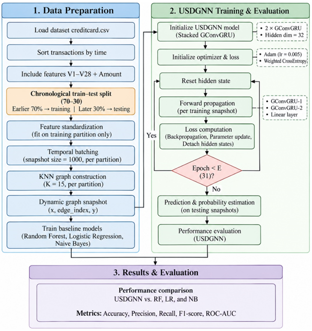
This framework is designed to address structural relations between transactions, time-related changes in behavioral patterns, and severe class imbalance, providing a realistic approach to fraud detection. Figure 1 illustrates the overall workflow of the proposed credit card fraud detection framework, depicting the complete processing pipeline from raw transaction acquisition to model evaluation and performance comparison.
Figure 1. The flow diagram of the Unified Spatiotemporal Dynamic Graph Neural Network (USDGNN) framework
The flow diagram illustrates the process of transferring transactional records into temporal graph snapshots, training a multi-layer GConvGRU-based USDGNN model, and ultimately comparing traditional ML models, including RF, NB, and LR, against the proposed USDGNN model. The flow diagram in Figure 1 details the temporal batching process, graph construction, dynamic learning and evaluation, and how these components integrate into a unified fraud detection framework. Below, we provide a brief illustration of the flow diagram; the next subsection details each stage.
The first step in the proposed fraud detection framework is to read raw credit card transactions and prepare them for preprocessing and temporal ordering. Then, the transactions are partitioned into snapshots of fixed size, where each snapshot is transformed into a graph using a similarity technique under the KNN algorithm. The resulting dynamic graph is then fed into the multi-layer GConvGRU-based USDGNN, which forces the model to learn temporally frequent instances.
To handle the class imbalance issues inherent in the credit card fraud detection dataset, a cost-sensitive method is adopted during the optimization. At the end of the framework, the proposed USDGNN’s performance is assessed and compared against traditional machine learning algorithms.
3.1 Dataset description and preprocessing
The credit card fraud detection dataset is used to evaluate the current work and is available on Kaggle. The dataset is released by the ULB, which reflects the real-world credit card transactions conducted by European cardholders over a period of a couple of consecutive days in September 2013 [25].
The overall dataset comprises 284807 transactions, including 492 instances labeled as fraudulent, representing a highly imbalanced proportion of 0.172% of the dataset entries. This poses a critical challenge for traditional ML algorithms and underscores the need to use advanced methods to address it.
To comply with privacy regulations, the original dataset attributes undergo Principal Component Analysis (PCA), resulting in 28 principal components named V1, V2, ..., V28. Due to security constraints, the dataset does not reflect any semantic correlation among the components. Nevertheless, two attributes remain in their original form: Time and Amount. Table 2 shows a sample of the dataset.
Table 2. Sample credit card fraud detection dataset
|
Time |
V1 |
V2 |
V8 |
Amt |
C |
|
406 |
-2.31 |
1.95 |
1.39 |
0.00 |
1 |
|
472 |
-3.04 |
-3.16 |
-0.07 |
529.00 |
1 |
|
0 |
-1.36 |
-0.07 |
0.10 |
149.62 |
0 |
|
1 |
-1.36 |
-1.34 |
0.25 |
378.66 |
0 |
First, order all transactions chronologically by the Time attribute. The ordered transaction stream is then divided chronologically into a 70% training partition containing the earlier transactions and a 30% testing partition containing the later transactions. This ordering is preserved throughout preprocessing, temporal snapshot generation, graph construction, model training, and evaluation so that the test partition represents transactions occurring after those used for model development.
Several characteristics of the chosen dataset make detecting fraud more difficult. First, the rate of fraudulent transactions is extremely low (0.172%), creating a class imbalance that may bias regular classifiers toward the majority class. Second, the transactions are ordered chronologically, which makes it possible to test temporal learning algorithms that will be able to detect behavioral changes. Finally, the features obtained by applying PCA and anonymizing the data retain their discriminatory power, making it unnecessary to use hand-crafted attributes.
To demonstrate the temporal events, let the stream of transactions be expressed as the following formula.
$\mathcal{J}=\left\{\left(x_i, y_i, t_i\right)\right\}_{i=1}^N$ (1)
where, $x_i$ denotes the feature vector of transaction $i, y_i$ is the binary class label $\{0,1\}$, and $t_i$ represents the timestamp of the transaction. The final dataset obtained is organized as follows:
$t_1 \leq t_2 \leq \cdots \leq t_N$
3.1.1 Feature selection
The model input consists of the PCA-transformed attributes (V1, …, V28) together with the Amount attribute. The Time attribute is retained only to establish chronological ordering and is excluded from the predictive feature matrix.
To avoid information leakage from future transactions, we standardize features after defining the chronological train–test partition. For each input feature, the mean and standard deviation are estimated exclusively from the training partition. The same training-derived parameters are subsequently applied to both the training and testing partitions. No statistics from the held-out test partition are used to fit the preprocessing transformation. The standard scale is employed, which is defined as the following equation:
$x^{\prime}=\frac{x-\mu}{\sigma}$ (2)
where, x denotes the original feature value, μ represents the mean of the feature, σ denotes its standard deviation, and x′ is the resulting standardized feature value.
After the chronological train–test partition and feature transformation are completed, temporal batching is performed independently within the training and testing partitions. Transactions in each partition retain their original chronological order and are divided into non-overlapping temporal snapshots of 1,000 transactions. The snapshot size is fixed throughout the experiments to maintain a consistent graph size and temporal batching scheme across successive GConvGRU inputs. However, 1,000 is a fixed experimental configuration rather than an empirically optimized temporal-window size. Thus, no temporal snapshot contains transactions from both the training and testing partitions, and the chronological boundary between model-development data and future evaluation data is preserved. As demonstrated in the flow diagram, each transaction is expressed by a distinct snapshot according to the following formula:
Assume that Sk represents the Kth snapshot:
$\mathcal{S}_k=\left\{x_{(k-1) B+1}, \ldots, x_{k B}\right\}$ (3)
where, B is equal to 1000, representing the snapshot size.
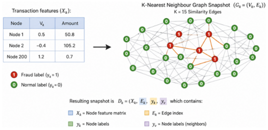
For each temporal snapshot, a KNN graph is constructed independently using k = 15. Each transaction within the snapshot is represented as a node, and edges are established according to feature-space similarity among transactions belonging to that snapshot only. Training graphs are therefore constructed exclusively from training transactions, whereas test graphs are constructed exclusively from transactions in the held-out chronological test partition. No KNN search or graph edge is allowed to cross the training–testing boundary. In mathematical terms, the graph snapshot can be defined as follows:
$\mathcal{G}_k=\left(\mathcal{V}_k, \mathcal{E}_k\right)$ (4)
where, $\mathcal{V}_k$ represents a transaction of snapshot k, and the edges are represented in the form as follows:
$e_{i j} \in \mathcal{E}_k|\Leftrightarrow| x_j \in \mathrm{KNN}\left(x_i\right)$ (5)
The KNN graph construction method maintains local similarity relationships while creating a sparse graph that is easy to handle for graph learning. It is suitable for detecting credit card fraud because fraudulent transactions tend to have locally similar behavior, even though they are very few compared to the rest of the dataset.
Each graph snapshot is represented in PyTorch Geometric as:
$\mathcal{D}_k=\left(X_k, E_k, y_k\right)$ (6)
where, $X_k$ is the feature vector of nodes, $E_k$ is the index of transaction edges, and $y_k$ contains classes of nodes. As an example of constructing a KNN graph for a single time point, see Figure 2, where every node is a transaction, while the edges represent similarity in the feature space for k = 15. This resulting graph, written as $(X_k, E_k, y_k)$ is used as input to the USDGNN.
Selecting the K value in KNN graph construction is critical because it directly affects graph connectivity and learning behavior. In this study, we set k to 15 to balance graph sparsity, local connectivity, and performance efficiency. Setting k to a small value limits information propagation and weakens graph connections, whereas a higher k may produce noisy connections in the graph. We empirically set the neighborhood size to k = 15 to balance graph sparsity, local connectivity, and computational efficiency.
Preliminary experiments indicated that this value produced stable graph structures while preserving sufficient neighborhood information for effective temporal graph learning within an adequate local neighborhood, enabling the USDGNN to learn meaningful similarities between patterns and reveal fraudulent transactions. Algorithm 1 simplifies the steps for constructing the KNN graph that serves as input to the USDGNN model.
|
Algorithm 1. Temporal batching and dynamic graph snapshot construction |
|
Input: Time-ordered transaction dataset $\boldsymbol{D}$, feature set $\boldsymbol{F}$, snapshot size $\boldsymbol{S}$, number of neighbors $\boldsymbol{K}$. Output: Dynamic graph snapshots $\left\{\boldsymbol{D}_1, \boldsymbol{D}_2, \ldots, \boldsymbol{D}_T\right\}$. Begin:
3.1 Construct the node feature matrix $X_t$ using $F$. 3.2 Build a KNN graph with $K$ nearest neighbors. 3.3 Generate the edge index $E_t$. 3.4 Assign node labels $y_t$. 3.5 Form the graph snapshot using $D_t=\left(X_t, E_t, y_t\right)$,
End. |
The training and testing graph snapshots generated through the leakage-controlled procedure described above constitute two chronologically separated graph sequences. Only the training sequence is used for model parameter optimization, whereas the later test sequence is retained exclusively for final performance evaluation. The generated graph snapshots constitute the sequential input to the USDGNN model, enabling recurrent graph learning across consecutive temporal windows.
3.2 Unified Spatiotemporal Dynamic Graph Neural Network architecture
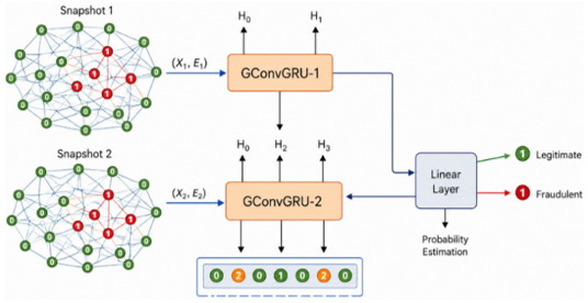
After dividing the chronologically ordered dataset into training and testing partitions, the model estimates preprocessing parameters from the training partition and independently transforms both partitions into temporal graph snapshots. The USDGNN is then trained exclusively on the training snapshot sequence to learn structural relationships within individual snapshots and temporal dependencies across consecutive training snapshots. The held-out chronological test snapshots are used only for final evaluation. Our proposed credit card fraud detection framework relies on a stacked GConvGRU, which captures dependencies related to transaction spatial characteristics and temporal dynamics across consecutive snapshots. In this work, the USDGNN includes two GConvGRU layers, each with a hidden layer of 32 units.
While regular GNN analyze graphs individually, GConvGRU improves on this by adding recurrence gates to the graph convolutional mechanism. This way, the information gathered from earlier graph snapshots can be used to influence the processing of later snapshots. In effect, the model not only captures spatial relationships within individual transaction graphs but also temporal relationships that define the evolution of transaction behavior.
Assume that
$\mathcal{D}_t=\left(X_t, E_t, y_t\right)$ (7)
Represent the snapshot of the graph at time t, where $X_t \in$ $\mathbb{R}^{N_t \times F}$ denotes the node feature array, $E_t$ is the edge, and $y_t$ is the class label. The updating of the hidden states of GConvGRU is defined as
$H_t=\operatorname{GConvGRU}\left(X_t, E_t, H_{t-1}\right)$ (8)
where, $H_{t-1}$ is the encoding of historical data from previous snapshots, and this is the core idea of “recurrent fashion learning” behind learning the evolving fraudulent behavior and eliminating the assumption that each transaction is an independent observation.
Figure 3. The Unified Spatiotemporal Dynamic Graph Neural Network (USDGNN) Architecture with Graph Convolutional Gated Recurrent Unit (GConvGRU) layers for credit card fraud detection
Figure 3 demonstrates the GDNN modeling and inference process. Referring to Figure 3, the first GConvGRU-1 layer receives each snapshot, denoted by $\left(X_{\mathrm{t}}, E_{\mathrm{t}}\right)$ and performs graph convolution, permitting the model to directly aggregate spatial correlation data from the neighboring transactions and maintain the temporal context utilizing hidden states, where the hidden state is updated according to the equation below:
$H_t^{(1)}=G C o n v G R U_1\left(X_t, E_t, H_{t-1}^{(1)}\right)$ (9)
The output of the first layer is fed to the second GConvGRU layer. The latter serves as a refinement node for representations by learning high-level temporal and relevant instances. The USDGNN model proposed herein can maintain transaction history while accommodating behavioral changes by spreading representations across consecutive graph snapshots. Learning through recurrence allows the model to distinguish fraudulent behavior from temporary changes in environmental behavior.
3.3 Handling imbalanced dataset
The credit card fraud dataset has a high-class imbalance, where frauds are just 0.172% of the entire dataset. To prevent the problem of optimization being biased towards the majority class, the paper uses cost-sensitive learning by incorporating the weighted cross-entropy loss function:
$L_{W C E}=-\frac{1}{N} \sum_{i=1}^N\left[w_0\left(1-y_i\right) \log \left(1-\hat{y}_i\right)+w_1 y_i \log \left(\hat{y}_i\right)\right.$ (10)
where, $y_i \in$ {0,1} is the ground-truth label, ŷᵢ is the predicted fraud probability, and w₀, w₁ are the class weights assigned to legitimate and fraudulent transactions, respectively. Rather than computing weights from inverse class frequencies, which would yield an extremely large minority weight given the severe class imbalance ratio in the training partition, we empirically set the class weights to w0 = 1.0 and w1 = 30.0 through preliminary experiments. This moderate positive class weight was selected to balance the precision–recall trade-off without causing the model to generate excessive false positives. These weights are implemented via PyTorch's CrossEntropyLoss with weight=torch. tensor ([1.0, 30.0]) and remain fixed throughout all training epochs.
In contrast, to ensure a fair comparison, classical machine learning models also address the imbalanced data problem. The LR and RF models are trained with balanced class weights, enabling them to mitigate class imbalance during optimization. Nevertheless, we included the NB model as a reference baseline without explicit class-imbalance correction.
To ensure clarity, Algorithm 2 outlines the proposed temporal credit card fraud detection method with USDGNN, including temporal snapshot creation, dynamic graph construction, and cost-sensitive USDGNN learning.
|
Algorithm 2. Temporal USDGNN-based credit card fraud detection |
|
Input: Credit card transaction dataset $\boldsymbol{D}$, snapshot size $\boldsymbol{B}$, KNN parameter $\boldsymbol{K}$, number of epochs $\boldsymbol{E}$. Output: Fraud probabilities and performance metrics. Process:
6.1 Perform forward propagation for each graph snapshot. 6.2 Compute the loss and update model parameters.
End. |
The computational complexity of the proposed USDGNN algorithm can be categorized into two main phases: graph construction and learning on temporal graphs. During pre-processing, graph construction maps each temporal snapshot to a KNN graph. However, for a snapshot with N transactions, the graph construction phase mainly depends on the nearest-neighbor search method, where each node connects to k other nodes, making the graph sparse. Since k remains constant, the number of edges scales with the number of transactions per snapshot.
In the training phase, the main computational expense comes from graph convolutions in the stacked GConvGRU blocks. This is because graph convolution operates on neighboring nodes rather than all combinations of nodes, so the computational complexity depends on the number of edges in the graph, not the square of the number of transactions.
3.4 Computational complexity analysis
Moreover, splitting the transaction flow into fixed-sized temporal snapshots lets the framework process data incrementally, avoiding the construction of a single graph containing all transactions. In addition, it makes the framework memory-efficient and scalable while retaining temporal relationships through recurrent graph learning. Thus, the USDGNN framework is well-suited for large-scale credit card fraud detection.
3.5 Evaluation metrics
The performance of the proposed temporal credit card fraud detection with USDGNN is evaluated using several numerical benchmark metrics, including accuracy, precision, recall, F1-score, and the Receiver Operating Characteristic (ROC) Area Under the Curve (AUC) visualization plot metric, which provides more comprehensive and reliable insight into fraud detection capability compared with accuracy. The numerical metrics are derived from a special numerical arrangement matrix called the Confusion Matrix (CM) [26]. The CM consists of four key values: True Positive (TP), True Negative (TN), False Positive (FP), and False Negative (FN).
The accuracy, precision, recall, and F1-score are derived from the CM and expressed in the following equations:
$\operatorname{Accuracy}~(A C)=\frac{(T P+T N)}{(T P+T N+F P+F N)}$ (11)
where, Accuracy (AC) denotes the proportion of correctly classified instances among all evaluated instances.
$\operatorname{Recall}~(\mathrm{R})=\frac{T P}{(T P+F N)}$ (12)
where, Recall (R), also known as Sensitivity or the True Positive Rate (TPR), measures the proportion of actual instances that are correctly identified by the model.
$\operatorname{Precision}~(P)=\frac{(T P)}{(T P+F P)}$ (13)
where, Precision (P) measures the proportion of instances predicted as fraudulent that are actually fraudulent.
$F 1-\operatorname{score}~(F)=\frac{2 \cdot R \cdot P}{(R+P)}$ (14)
where, F1-score (F) is the harmonic average of precision and recall, balancing both in their ability to correctly detect the fraud cases while at the same time avoiding as many false positives or false negatives as possible.
To ensure a leakage-free chronological evaluation, all reported experiments use the same 70–30 chronological partition defined in Section 3. We use transactions in the earlier 70% for model development, while retaining the later 30% as the held-out test set. We estimate feature-standardization parameters exclusively from the training partition and apply them unchanged to the test partition. Temporal batching and KNN graph construction are performed independently within each partition, ensuring that no preprocessing statistics, temporal snapshots, or graph edges cross the training–test boundary. The baseline classifiers are trained and evaluated using the same chronological training and test partitions to ensure a consistent comparison with USDGNN.
4.1 Testing environment
The experiment in this study assessed the efficacy of the USDGNN model framework for detecting fraud in credit card transactions within the constraints of recourse. All experiments were carried out on a personal computer to prove the practical feasibility of the research. Table 3 presents the full hardware and software specifications used in the experiment.
Table 3. Experimental testing environment
|
Category |
Configuration |
|
Hardware |
Intel® Core™ i5 PC, 8 GB RAM |
|
Operating System |
Windows 11 |
|
Environment |
Python, Anaconda, Jupyter Notebook |
|
Libraries |
pandas, NumPy, scikit-learn, PyTorch, PyTorch Geometric, PyTorch Geometric Temporal |
|
Model Architecture |
Graph Convolutional Gated Recurrent Unit (GConvGRU) |
In this scenario, we not only provide a replicable environment but also demonstrate the usability of the suggested USDGNN framework for large-scale operations without requiring supercomputing hardware.
4.2 Results
We obtained all reported test results from the held-out final 30% of the chronologically ordered transaction stream. Model fitting, preprocessing-parameter estimation, and training-stage optimization were restricted to the earlier 70% training partition. The test partition was not used to estimate standardization parameters or optimize model parameters.
This section presents a detailed evaluation of experiments conducted with the proposed USDGNN framework for credit card fraud detection, highlighting the model's efficiency compared with traditional ML models (e.g., RF, LR, and NB). In this regard, the comparison evaluates the models' classification performance in the critical case of an unbalanced dataset and the need to capture and track dynamic transactions. In addition to numerical metric evaluations, the results include visualization metrics to evaluate classification efficiency, including ROC-AUC plots for both USDGNN and traditional ML models.
The proposed USDGNN-based credit card fraud detection model remains consistently stable during training. This stability is reflected in the loss evolution during training, where the loss decreases from 0.2854 at epoch 0 to 0.0067 at the last epoch (i.e., epoch 30). Table 4 shows the classification performance of the proposed temporal credit card fraud detection with USDGNN versus the classical baseline classifiers (e.g., RF, LR, and NB).
Table 4. Evaluation metrics comparison of Unified Spatiotemporal Dynamic Graph Neural Network (USDGNN) and baseline traditional machine learning (ML) models
|
Model |
Accuracy |
Precision |
Recall |
F1-Score |
|
Random Forest (RF) |
0.9987 |
0.9189 |
0.7727 |
0.8395 |
|
Logistic Regression (LR) |
0.9878 |
0.2622 |
0.9773 |
0.4135 |
|
Naïve Bayes (NB) |
0.9786 |
0.1680 |
0.9773 |
0.2867 |
|
USDGNN |
0.9991 |
0.8478 |
0.8667 |
0.8571 |
All models show fairly good accuracy, but this is due to the natural class imbalance in the credit card fraud detection dataset; however, accuracy is not a dependable measure for fraud detection. In many similar cases, classification algorithms achieve high accuracy by favoring the majority target class and largely ignoring the minority target class. Thus, precision, recall, and F1-score measures are quite informative evaluation criteria that can be used to make fair comparisons.
Among the evaluated models, USDGNN achieved the highest F1-score of 0.8571, reflecting the strongest observed balance between precision and recall in the reported test split. Random Forest achieved the highest precision of 0.9189 but lower recall of 0.7727, whereas USDGNN achieved precision of 0.8478 and recall of 0.8667. Thus, the reported results do not indicate that USDGNN is uniformly superior across all metrics; rather, they show that USDGNN provides the highest F1-score and a comparatively balanced precision–recall profile among the evaluated classifiers.
The LR and NB models achieve extremely high recall; however, this high confidence comes at the cost of very low precision. Consequently, the F1-score recorded poor values. This limitation offers a crucial insight and highlights the limitations of linear and probabilistic algorithms on highly imbalanced datasets, where the model is biased toward predicting the majority target class. Our proposed USDGNN addresses this issue by constructing and exploiting graph neighborhood data, learning and modeling temporal correlations among transaction snapshots, and incorporating cost-sensitive learning throughout the optimization process. Consequently, within the reported test split, USDGNN achieved a comparatively balanced precision–recall profile, reflecting its ability to detect fraudulent transactions while limiting false-positive predictions relative to the high-recall baseline models.
Figure 4 demonstrates the ROC curves of the proposed USDGNN and traditional baseline classification models. USDGNN achieved an ROC-AUC of 0.9913, indicating strong discrimination between fraudulent and legitimate transactions in the reported test set. However, RF and LR achieved higher overall AUC values. Therefore, the ROC analysis should be interpreted together with the precision, recall, and F1-score results rather than as evidence of uniform superiority of USDGNN across all evaluation criteria.
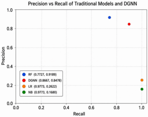
Figure 5 shows the precision-recall distribution of the evaluated models. This evaluation shows each model's effectiveness under an imbalanced class distribution. The RF model overruns the high-precision region, reflecting modest fraud detection that minimizes false alarms but abandons some detection capability.
Figure 4. ROC curves comparing the proposed Unified Spatiotemporal Dynamic Graph Neural Network (USDGNN) with baseline classifiers
Figure 5. Precision–Recall comparison of the evaluated classifiers
The LR and NB reside in the high-recall but low-precision region, demonstrating aggressive fraud-detection behavior that classifies many legitimate transactions as fraudulent. The proposed USDGNN occupies a comparatively balanced region of the precision–recall space, with a recall of 0.8667 and a precision of 0.8478. This position is consistent with its F1-score of 0.8571 and distinguishes its operating behavior from RF, which favors precision, and LR and NB, which favor recall at the expense of substantially lower precision. Table 5 lists selected studies on fraud detection, along with their techniques, data used, and performance results.
Since the studies summarized in Table 5 were conducted using different datasets, graph construction strategies, preprocessing procedures, and experimental protocols, the reported performance metrics are presented for contextual reference only and should not be interpreted as a direct empirical comparison with the proposed USDGNN framework. Instead, Table 5 illustrates the methodological evolution of fraud detection techniques from conventional machine learning methods to graph-based and temporal graph learning approaches, thereby motivating the development of the proposed USDGNN framework.
Table 5. Summary of representative credit card fraud detection studies and their reported performance
|
Study |
Data |
Accuracy |
F1-Score |
Model |
|
[14] |
Bench. |
- |
- |
ML |
|
[15] |
Mixed |
97–99 |
0.89 |
Ens.-ML |
|
[17] |
Private |
~78 |
~0.86 |
GNN+AE |
|
[18] |
Synth. |
97 |
0.86 |
ED-GNN |
|
[20] |
Yelp/Amaz. |
- |
0.72 |
CaT-GNN |
|
USDGNN |
ULB |
99.91 |
0.857 |
Temp. DGNN |
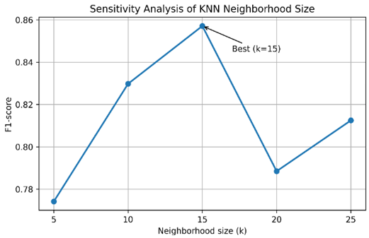
4.3 Sensitivity analysis of the K-Nearest Neighbors neighborhood size
To examine USDGNN's sensitivity to the KNN neighborhood size, we evaluated different values of k in the graph-generation process while keeping the temporal snapshot size fixed at 1,000 transactions. Accordingly, this analysis evaluates sensitivity to neighborhood connectivity only and should not be interpreted as a joint sensitivity analysis of all graph-construction parameters. The choice of neighborhood size directly controls the connectivity in the graph by determining how many transaction neighbors are connected to a single node within a particular temporal window; since information propagates throughout the graph during graph convolution via its topology, a suitable choice of k should provide balanced performance across all classes.
To examine the impact of k, the proposed USDGNN was trained and evaluated across neighborhood sizes of k = 5, 10, 15, 20, and 25, keeping all other parameters, including snapshot size, network architecture, optimizer, learning rate, and class weight settings identical across all configurations. It must be noted that, due to the absence of a separate validation set in the current experimental design, all reported sensitivity results were obtained by evaluating each k configuration directly on the same held-out chronological 30% test partition used for the main performance comparison in Section 4.2. Consequently, the selection of k = 15 as the reported best configuration was based on its observed test set F1-score performance rather than on an independent validation set. This represents a limitation of the current sensitivity analysis, the selected k value may be optimistically tuned to the specific test partition, and the reported performance differences across k values should therefore be interpreted as exploratory observations rather than as statistically validated conclusions. A rigorous future evaluation should employ a dedicated held-out validation partition, for example, a chronological 70/15/15 train, validation, test split, to select the optimal k independently of the final test set, followed by a single confirmatory evaluation on the held-out test partition. The sensitivity results are presented in Table 6.
From Table 6, we see that neighborhood size significantly affects the learning behavior of the proposed USDGNN. With a relatively small neighborhood (k = 5), the graph created is sparse, and information can’t easily propagate among neighborhood transactions. As a result, the model achieves relatively high accuracy but lower precision and F1-score.
Setting the neighborhood size to k = 10 significantly improves the graph's connectivity, thereby substantially improving both precision and F1-score. The maximum F1-score (0.8571) was observed at k = 15, accompanied by a reasonable precision (0.8478) and recall (0.8667), demonstrating a reasonable balance between sparsity and graph neighborhood connectivity in the USDGNN, allowing the capture of relevant structural connections without introducing excessive irrelevant information. Increasing the neighborhood size to k = 20 yields maximum recall (0.9111), whereby a larger fraction of fraudulent transactions is detected.
Table 6. Sensitivity analysis of the K-Nearest Neighbors (KNN) neighborhood size used for graph construction
|
Neighborhood Size (k) |
Accuracy |
Precision |
Recall |
F1-Score |
|
5 |
0.9986 |
0.7500 |
0.8000 |
0.7742 |
|
10 |
0.9989 |
0.7959 |
0.8667 |
0.8298 |
|
15 (Proposed) |
0.9991 |
0.8478 |
0.8667 |
0.8571 |
|
20 |
0.9985 |
0.6949 |
0.9111 |
0.7885 |
|
25 |
0.9988 |
0.7647 |
0.8667 |
0.8125 |
However, this enhancement in recall comes at the cost of a significant drop in precision (0.6949) due to the addition of false-positive predictions from high information transmission between unrelated transactions, which builds denser graphs. Increasing the neighborhood size to k = 25 partially recovers precision, but the F1-score remains lower than at k = 15. Thus, this indicates that densely connected graphs are not always the solution for improving fraud detection.
Figure 6 shows the effect of the KNN neighborhood size on the performance of the proposed USDGNN. In this scenario, the USDGNN performs optimally at k = 15, as the balance between graph sparseness and neighborhood size is optimal; larger k yields a denser graph structure, degrading the classifier's performance, while lower k reduces propagation.
Figure 6. Effect of the K-Nearest Neighbors (KNN) neighborhood size on the performance of the proposed Unified Spatiotemporal Dynamic Graph Neural Network (USDGNN)
Although a larger graph allows more structural information to propagate, it also includes numerous edges between unrelated transactions, introducing additional noise. It is worth noting that there is a slight performance improvement when increasing k from 20 to 25; this suggests that USDGNN performs well over a relatively broad range of k; nonetheless, it does not outperform our configuration. The results indicate that USDGNN maintains competitive performance across the evaluated neighborhood settings, yielding the highest observed F1-score.
This conclusion is limited to variation in neighborhood size because the temporal snapshot size remained fixed at 1,000 transactions throughout the analysis.
4.4 Discussion
The experimental results indicate that the evaluated classifiers exhibit different performance trade-offs. USDGNN achieved the highest F1-score (0.8571) and accuracy (0.9991), with precision (0.8478) and recall (0.8667). In contrast, Random Forest achieved the highest precision of 0.9189 but a lower recall of 0.7727, whereas Logistic Regression and Naïve Bayes achieved higher recall values of 0.9773 but substantially lower precision. Accordingly, USDGNN should be interpreted as providing the strongest observed F1-based precision–recall balance among the evaluated models rather than as outperforming every baseline on every metric.
These results are also confirmed by the ROC analysis. USDGNN had an AUC of 0.9913 and an optimal operating point in the low false-positive region, which is critical for any fraud detection system to be practically usable. Furthermore, the training loss showed a gradual decrease from 0.2854 in the initial epochs to 0.0067 by the end of 30 epochs, supporting the stability and effectiveness of convergence. In addition, the analysis of sensitivity to neighborhood size indicated that the value k = 15 yielded the highest observed F1-score of 0.8571 compared to other values of k tested, i.e., k = 5, 10, 15, 20, and 25. Nevertheless, it must be pointed out explicitly that this choice is made using test set evaluation rather than using a separately reserved validation set since there is no validation set specified for the current experiment. Therefore, this conclusion is to be considered as sensitivity exploration rather than validation of the optimal configuration.
The outcomes are consistent with the most recent progress reported in the literature on graph-based fraud detection methods. Conventional machine learning methods suffer significant performance degradation under severe class imbalance because transactions are treated as independent tabular records without modeling structural or relational dependencies [14]. While ensemble-based approaches can enhance classification accuracy, they remain limited in their ability to capture structural relationships among transactions [15]. Furthermore, although resampling techniques such as SMOTE combined with ensemble classifiers can partially address class imbalance, they fail to capture the temporal dynamics of evolving fraudulent behavior [16].
Some of these limitations have been partially addressed through graph-based approaches. An Encoder-Decoder Graph Neural Network (EDGNN) architecture applied to the synthetic Sparkov dataset achieved an F1-score of approximately 0.86 and an AUC of 0.92 [18]. The proposed USDGNN obtained a comparable F1-score of 0.8571 when evaluated on the highly imbalanced real-world ULB credit card dataset, demonstrating that dynamic graph learning can be applied effectively to more challenging real transaction data. Among temporal graph learning approaches, the CaT-GNN framework, which incorporates causal and temporal graph modeling, reported an F1-score of 0.721 [20], while the Temporal Graph Network (TGN)-based approach for online payment fraud detection reported an F1-score of 0.4523 with an AUC of 0.7255 [19]. In contrast to these approaches, the proposed USDGNN provides a unified end-to-end framework that combines chronological transaction ordering, KNN-based temporal graph construction, stacked GConvGRU learning, and cost-sensitive optimization. However, these comparisons should be regarded as contextual validation only, not as direct empirical comparisons, because the referenced studies used different datasets, graph construction strategies, preprocessing techniques, evaluation methods, and fraud distributions.
Several observations can be drawn from the reported experiments. First, under the evaluated chronological split, temporal graph learning produced a favorable precision–recall trade-off relative to the traditional machine learning baselines, as reflected by the highest observed F1-score for USDGNN. USDGNN models structural relationships among similar transactions together with temporal relationships across sequential transaction snapshots, whereas the evaluated conventional classifiers operate on tabular transaction features without explicit graph-based temporal modeling. Additionally, USDGNN models structural relationships between similar transactions and temporal relationships between sequential transaction snapshots, whereas traditional classifiers only model the sequential transactions. This enables the framework to incorporate information from preceding transaction snapshots when classifying transactions in subsequent snapshots. Second, the severe class imbalance in the ULB dataset is addressed through cost-sensitive optimization rather than resampling. By assigning a larger loss contribution to misclassified minority fraudulent transactions, the training objective reduces the model's tendency to favor the majority legitimate class while preserving the original class distribution. Third, the neighborhood sensitivity analysis is consistent with this: it validates the importance of graph construction on the overall performance. The neighborhood size k = 15 is large enough to capture the structure of the graph yet small enough to avoid the “graph density” seen with larger values of k, maximizing the F1-score. Finally, the proposed framework is practical and scalable for large-scale fraud detection while keeping learning stable during training by combining KNN-based graph construction with recurrent graph convolution.
Although the proposed USDGNN framework showed promising results in terms of performance, the following limitations should be noted. The experiments used only the public ULB credit card fraud dataset, collected over a short period and anonymized with PCA-transformed features. Hence, the applicability of the proposed framework to other financial institutions, geographical regions, or new fraud techniques is an important issue that needs to be explored.
Second, the temporal snapshot size was fixed at 1,000 transactions throughout the experiments. Although a sensitivity analysis was conducted for the KNN neighborhood size and yielded the highest observed F1-score, an equivalent sensitivity analysis of the temporal snapshot size was not performed. Because snapshot size directly affects graph size, temporal granularity, and the amount of structural information available within each graph, the selected value of 1,000 should be regarded as a fixed design choice rather than an empirically optimized parameter. Future work should evaluate multiple snapshot sizes and jointly examine their interaction with the KNN neighborhood size. Third, only one chronological train–test split was examined, and repeated training runs, confidence-interval estimation, and statistical significance testing were not conducted. Consequently, the reported differences should be interpreted as observed performance differences under the present experimental setting rather than as statistically significant improvements. Future evaluations using multiple independent runs, additional datasets, confidence intervals, and appropriate hypothesis tests are required to establish the statistical reliability and generalizability of the observed performance differences.
Lastly, only three traditional machine learning baselines (random forest, logistic regression, and naïve Bayes) were included and evaluated comparatively. The USDGNN can be compared with other state-of-the-art GNN architectures, graph attention networks, and recent temporal graph learning models in future work using the same experimental setup and conditions. Moreover, incorporating real-time streaming transaction analysis, adaptive graph generation, explainable graph learning, and online continual learning would further enhance its use in real-world financial fraud detection systems.
This paper introduced a temporal USDGNN framework for credit card fraud detection to address the limitations of classical machine learning algorithms in modeling dynamic transactions and evolving fraud behavior over time. Our proposed framework first represents transactions in chronological order as a sequence of KNN-based graph snapshots, then applies stacked GConvGRU layers to jointly learn transaction-to-transaction structural information and temporal transitions. We further introduced a cost-sensitive learning strategy to optimize fraud detection under severe class imbalance. Experimental results on the publicly available ULB credit card fraud dataset showed that USDGNN achieved 99.91% accuracy, 84.78% precision, 86.67% recall, and an F1-score of 85.71%, which was the highest F1-score among the evaluated models. Random Forest achieved higher precision, whereas Logistic Regression and Naïve Bayes achieved higher recall. Thus, within the reported chronological test split, USDGNN's main performance advantage was its more balanced precision–recall trade-off rather than uniform superiority across all evaluation metrics. Furthermore, the neighborhood-size sensitivity analysis showed that achieved the highest observed F1-score among the evaluated KNN settings under the fixed snapshot size of 1,000 transactions. This supports the selected neighborhood configuration for the present experimental setting, while the influence of temporal snapshot size remains to be investigated. These findings suggest that combining graph-based representations, temporal modeling, and cost-sensitive learning can provide a useful precision–recall trade-off for fraud detection under the evaluated experimental conditions. Yet, there are several limitations to this work. First, the experiments were conducted on one publicly available benchmark dataset; therefore, additional experiments on large-scale real-world financial transactions data should be performed in order to confirm the generalization ability of the algorithm. Furthermore, the proposed approach assumes fixed parameters for temporal snapshot creation and the size of the KNN neighborhood, which may not be appropriate for different transaction environments. In addition, our approach works offline; that is, the initial set of historical graph snapshots is created before training begins rather than from the transaction stream. Future work includes adapting the proposed framework for online dynamic graph learning for real-time fraud detection and developing a graph construction technique to automatically adjust parameters related to the KNN neighborhood and temporal snapshots. It would also be worthwhile to incorporate graph attention mechanisms, self-supervised graph representation learning, and other advanced temporal GNN architectures to detect new and more complex forms of fraud.
[1] Kumar, A. (2024). E-Commerce: Boon for global financial market. International Journal of Innovations in Science, Engineering and Management, 2: 115-121. https://ijisem.com/journal/index.php/ijisem/article/view/112.
[2] Shuai, Q., Huang, R., Liu, J., Zhang, L. (2025). Research prospect of e-commerce and financial payment. In Handbook of E-commerce in China, Singapore: Springer Nature Singapore, pp. 233-251. https://doi.org/10.1007/978-981-96-7629-3_15
[3] Goudar, S.I., Bhowmik, B. (2024). Intelligent fraud detection techniques in credit card and internet banking. In 2024 International Conference on Communication, Control, and Intelligent Systems (CCIS), Mathura, India, pp. 1-6. https://doi.org/10.1109/CCIS63231.2024.10932113.
[4] Reurink, A. (2018). Financial fraud: A literature review. Journal of Economic Surveys, 32(5): 1292-1325. https://doi.org/10.1111/joes.12294
[5] Saluja, S. (2024). Identity theft fraud-major loophole for FinTech industry in India. Journal of Financial Crime, 31(1): 146-157. https://doi.org/10.1108/JFC-08-2022-0211
[6] Seera, M., Lim, C.P., Kumar, A., Dhamotharan, L., Tan, K.H. (2024). An intelligent payment card fraud detection system. Annals of Operations Research, 334(1-3): 445-467. https://doi.org/10.1007/s10479-021-04149-2
[7] Guers, K., Chowdhury, M.M., Rifat, N. (2022). Card skimming: A cybercrime by hackers. In 2022 IEEE International Conference on Electro Information Technology (eIT), Mankato, MN, USA, pp. 575-579. https://doi.org/10.1109/eIT53891.2022.9813890
[8] Santoso, R., Gunawan, A.A. (2024). Detecting account takeover (ATO) in fintech companies using machine learning. In 2024 6th International Conference on Cybernetics and Intelligent System (ICORIS), Surakarta, Indonesia, pp. 1-6. https://doi.org/10.1109/ICORIS63540.2024.10903690
[9] Compagnino, A.A., Maruccia, Y., Cavuoti, S., et al. (2025). An introduction to machine learning methods for fraud detection. Applied Sciences, 15(21): 11787. https://doi.org/10.3390/app152111787
[10] Shanbhog, N.R., Totad, K.S., Hanchinal, A.R., Bidargaddi, A.P. (2024). Fraud detection in financial transactions using deep learning approach: A comparative study. In 2024 5th International Conference for Emerging Technology (INCET), Belgaum, India, pp. 1-7. https://doi.org/10.1109/INCET61516.2024.10593486
[11] Dastidar, K.G., Caelen, O., Granitzer, M. (2024). Machine learning methods for credit card fraud detection: A survey. IEEE Access, 12: 158939-158965. https://doi.org/10.1109/ACCESS.2024.3487298
[12] Rasul, I., Shaboj, S.I., Rafi, M.A., Miah, M.K., Islam, M.R., Ahmed, A. (2025). Detecting financial fraud in real-time transactions using Graph Neural Networks and anomaly detection techniques. Journal of Economics, Finance and Accounting Studies, 6(1): 131-142. https://doi.org/10.32996/jefas.2024.6.1.13
[13] Cai, L., Chen, Z., Luo, C., et al. (2021). Structural temporal Graph Neural Network for anomaly detection in dynamic graphs. In Proceedings of the 30th ACM International Conference on Information & Knowledge Management, Gold Coast, Queensland, Australia, pp. 3747-3756. https://doi.org/10.1145/3459637.3481955
[14] Bhattacharyya, S., Jha, S., Tharakunnel, K., Westland, J.C. (2011). Data mining for credit card fraud: A comparative study. Decision Support Systems, 50(3): 602-613. https://doi.org/10.1016/j.dss.2010.08.008
[15] Alrasheedi, M.A. (2025). Enhancing fraud detection in credit card transactions: A comparative study of machine learning models. Computational Economics, 68: 779-805. https://doi.org/10.1007/s10614-025-11071-3
[16] Sulaiman, S.S., Nadher, I., Hameed, S.M. (2024). Credit card fraud detection challenges and solutions: A review. Iraqi Journal of Science, 65(4): 2287-2303. https://doi.org/10.24996/ijs.2024.65.4.42
[17] Alarfaj, F.K., Shahzadi, S. (2025). Enhancing fraud detection in banking with deep learning: Graph Neural Network and autoencoders for real-time credit card fraud prevention. IEEE Access, 13: 20633-20646. https://doi.org/10.1109/ACCESS.2024.3466288
[18] Cherif, A., Ammar, H., Kalkatawi, M., Alshehri, S., Imine, A. (2024). Encoder-decoder graph neural network for credit card fraud detection. Journal of King Saud University-Computer and Information Sciences, 36(3): 102003. https://doi.org/10.1016/j.jksuci.2024.102003
[19] Saldaña-Ulloa, D., De Ita Luna, G., Marcial-Romero, J.R. (2024). A temporal graph network algorithm for detecting fraudulent transactions on online payment platforms. Algorithms, 17(12): 552. https://doi.org/10.3390/a17120552
[20] Duan, Y., Zhang, G., Wang, S., et al. (2024). CaT-GNN: Enhancing credit card fraud detection via causal temporal Graph Neural Network. arXiv preprint arXiv:2402.14708. https://doi.org/10.48550/arXiv.2402.14708
[21] Motie, S., Raahemi, B. (2024). Financial fraud detection using graph neural networks: A systematic review. Expert Systems with Applications, 240: 122156. https://doi.org/10.1016/j.eswa.2023.122156
[22] Saeed, M.S., Mustafa, M.W., Sheikh, U.U., Jumani, T.A., Mirjat, N.H. (2024). Deep learning for credit card fraud detection: A review of algorithms, challenges, and solutions. IEEE Access, 12: 96893-96910. https://doi.org/10.1109/ACCESS.2024.3426955
[23] Cheng, D., Zou, Y., Xiang, S., Jiang, C. (2025). Graph neural networks for financial fraud detection: A review. Frontiers of Computer Science, 19(9): 199609. https://doi.org/10.1007/s11704-024-40474-y
[24] Li, E., Chen, M., Xiang, S., Chen, L. (2025). Graph learning-empowered financial fraud detection: Progress and future directions. Intelligent Computing, 4: 0146. https://doi.org/10.34133/icomputing.0146
[25] Dal Pozzolo, A., Caelen, O., Johnson, R.A., Bontempi, G. (2015). Calibrating probability with undersampling for unbalanced classification. In 2015 IEEE Symposium Series on Computational Intelligence, Cape Town, South Africa, pp. 159-166. https://doi.org/10.1109/SSCI.2015.33
[26] Abdul Salam, M., Fouad, K.M., Elbably, D.L., Elsayed, S.M. (2024). Federated learning model for credit card fraud detection with data balancing techniques. Neural Computing and Applications, 36: 6231-6256. https://doi.org/10.1007/s00521-023-09410-2