Muhammad Khamim Asy’ari*![]() | Vinar Shinta Saitama Sitanggang | Kevin Bestian Ginting
| Vinar Shinta Saitama Sitanggang | Kevin Bestian Ginting![]()
© 2025 The authors. This article is published by IIETA and is licensed under the CC BY 4.0 license (http://creativecommons.org/licenses/by/4.0/).
OPEN ACCESS
The use of solar energy as electrical energy in Indonesia is still relatively small, accounting for 0.15GWp of a total of 207.8GWp capacity. The sustainability of renewable energy in Indonesia is an important aspect towards national energy security and one of the efforts is to create a real-time reliability monitoring system. Reliability is an important factor in the longevity of the components of a power plant. The purpose of this research is to create a real-time reliability monitoring system for a solar power plant (SPP) which is developed through two stages, modeling the SPP system and designing a reliability system. The SPP system model was built using an artificial neural network (ANN) which uses time and previous measurement data as input and three lags as variations. Measurement data is divided into training data and testing data with a ratio of 70:30. The ANN model for the reliability system is developed based on failure detection, which occurs when the predicted value deviates from the actual measurement by more than five percent. Each occurrence of failure will be detected and entered into Benard's approximation to determine the value of reliability. The results of the ANN model for the most accurate prediction system are achieved by using time and lag-3 voltage data as inputs. The resulting MSE value is 8.963×10⁻³ for training data and 9.533×10⁻³ for testing data. The SPP reliability value was 0.683 in the first year and continued to decrease by 0.376 in the second year. Preventive maintenance needs to be done when the reliability reaches 0.55 with a maintenance interval of 21 months.
anomaly detection, artificial neural network, reliability, solar power plant, voltage
The demand for electrical energy in Indonesia continues to rise. The State Electricity Company reported that national electricity consumption in 2018 was 232,296 TWh and is expected to grow by 5.1 percent annually. However, energy sources are still dominated by coal and fossil fuels by 59,6 percent [1]. However, the energy supply remains heavily dependent on coal and fossil fuels, accounting for 59.6 percent of the total energy mix 111. In response, the government is transitioning to renewable energy sources to reduce CO₂ emissions, with solar energy being a promising alternative.
Indonesia has significant solar energy potential [1]. Indonesia has significant solar energy potential. The National Energy General Plan (2017) estimates a generation capacity of 207.89GW, yet the installed capacity remains far below the target, reaching only 0.15GWp out of the 6.5GW target for 2025 [2]. The data shows that the energy produced by SPP is still far below the target. Of course, this still far-reaching level of achievement was triggered by several challenges.
The challenges of developing renewable energy can be seen from the problems in the form of investment costs, access to efficient technology, access to cheap funding, and reasonable selling prices or economic prices [3]. The biggest challenges in the development of renewable energy, especially in the development of SPPs, are economy and efficiency. Solar Power Plants (SPPs) are highly demanded as an energy source because they generate electricity in an environmentally friendly and cost-effective way, utilizing the unlimited potential of solar energy [4]. However, despite their advantages, SPPs still face technical and operational challenges that must be addressed to ensure consistent reliability and performance. A study of 23 renewable energy development projects across 17 countries found that almost 21 percent of the projects failed, and only 48 percent remained fully functional over time. This is largely due to a lack of responsibility, inadequate maintenance, and the use of low-quality technologies that compromise the reliability and capability of the systems in the long term [5]. Unanticipated failures that prolong downtime periods further worsen the situation and negatively impacting the financial performance of the investment [6]. In response to these challenges, one important effort is the development of a real-time reliability monitoring system, aimed at ensuring the sustainable performance of solar power plants. Reliability of renewable energy systems plays a significant role in optimizing decisions in design and economical operation over a long period of time [7].
Reliability is the probability of an item to be able to carry out the specified function, under certain operating conditions and environment for a specified period of time [8]. This malfunction has the potential to affect the efficiency of system performance which in turn will also increase maintenance costs at the level of severe damage. Several studies have concluded that energy and maintenance are generally the main factors affecting production costs. A real-time reliability monitoring system could address these issues by enabling early detection of failures, preventing total system breakdowns, and minimizing downtime.
Research on monitoring the reliability levels of Solar Power Plants (SPP) has been extensively conducted by several researchers. One method used is the control chart. A control chart is a diagram that provides an image of the behavior of a process. The determination of the control chart is based on the calculation of statistical values computed from the entire sample. In a control chart, limits are set where a process can be said to deviate, consisting of the Upper Control Limit (UCL) and the Lower Control Limit (LCL). Reliability values are calculated using an exponential distribution obtained based on the failure rate by considering the number of data points deviating from the set limits. The results show that the reliability value decreases to 0.55 after the SPP has been operating for 22 days [9]. Another method used involves a control chart with a Weibull distribution, which can represent many Probability Density Functions (PDF). The system reliability value of 0.3 occurs at an operational time of 5 days [10]. Reliability calculations for solar panels use the beta distribution and binomial distribution with a data working life of 17 years. The results show that reliability decreases from 100% at 12 years of working life to 2.5% at 17 years of working life [11]. Another study also uses the Reliability Block Diagram (RBD) approach with components such as Balance of System (BOS), inverter, Photovoltaic (PV) module, converter, and storage system. Reliability calculations are based on each subsystem. The reliability of the PV subsystem is 0.7956 after 10 years and 0.5036 after 30 years. The best Probability Density Function (PDF) for solar modules is the exponential distribution [12].
While previous research has explored various methods for assessing solar power plant (SPP) reliability, most approaches rely on offline statistical analyses, such as control charts, Weibull distributions, beta-binomial models, and Reliability Block Diagrams (RBDs). These methods provide valuable insights into system performance but lack real-time monitoring capabilities, limiting their ability to detect failures promptly. This study addresses this gap by proposing a real-time reliability monitoring system for SPPs. Unlike existing approaches, the proposed system enables continuous assessment of reliability metrics, allowing for early detection of potential failures and faster decision-making to optimize maintenance strategies [12]. By integrating real-time data acquisition and analysis, this research enhances the operational efficiency of SPPs, reduces maintenance costs, and contributes to the broader effort of improving the reliability and sustainability of solar energy systems.
The research method consists of six stages, namely data collection, data processing, data testing, SPP system modeling, model testing, anomaly detection design, and reliability monitoring design.
2.1 Data collecting
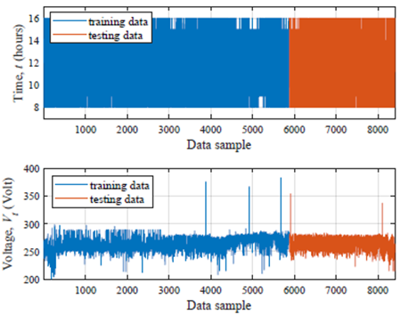
The data used is voltage measurement data from the solar power plant located at the Pandansimo Hybrid Power Plant, Bantul, Yogyakarta. The data consists of measurement results collected over a period of 5 years. Nine measurements are taken daily at one-hour intervals, from 08:00 to 16:00 GMT+7.
2.2 Data processing
Voltage measurement data is graphed based on time. The measurement data is also carried out by separating outliers using a box plot. The data is divided into two parts, namely training data and test data with a ratio of 70:30. The training data is used to obtain the weight and bias values of the ANN model and the test data is used to test the ANN model obtained previously.
2.3 Data testing
The data were tested using the correlation test, autocorrelation function (ACF) test, and partial autocorrelation function (PACF) test. The correlation test aims to get the value of the relationship between the independent variables and one dependent variable. The Pearson correlation test equation is shown in Eq. (1) [13, 14].
${{r}_{xy}}=\frac{n\sum\limits_{i=1}^{n}{x}y-\left( \sum\limits_{i=1}^{n}{x} \right)\left( \sum\limits_{i=1}^{n}{y} \right)}{\sqrt{\left\{ n\sum\limits_{i=1}^{n}{{{x}^{2}}}-{{\left( \sum\limits_{i=1}^{n}{x} \right)}^{2}} \right\}\left\{ n\sum\limits_{i=1}^{n}{{{y}^{2}}}-{{\left( \sum\limits_{i=1}^{n}{y} \right)}^{2}} \right\}}}$ (1)
ACF is a linear relationship between time series data x(i) and x(i-1) with the aim of identifying the model and the stationarity of the data in mean and covariance [15]. The ACF equation is shown in Eq. (2).
${{\rho }_{k}}=\frac{\sum\limits_{i=k+1}^{N}{(y(}i)-\bar{y})(y(i-k)-\bar{y})}{\sum\limits_{i=1}^{N}{(y(}i)-\bar{y}{{)}^{2}}}$ (2)
ρk is the autocorrelation function, y(i) is the i-th measurement data, and i is the time lag which refers to the delay or shift in time-series data, meaning that past values of a variable are used as inputs to predict future values.
PACF is the correlation between x(i) and x(i-1) after removing any linear dependence or x(t) and x(t-h). This coefficient is denoted ϕhh with a different, h [13]. If x(t) is a normally distributed time series, then:
${{\phi }_{hh}}=\operatorname{cor}\left( {{X}_{t}},{{X}_{t-h}}\mid {{X}_{t-1}},{{X}_{t-2}},\ldots ,{{X}_{t-h+1}} \right)$ (3)
A common method for determining PACF is to use the following Yule-Walker Eq. (4).
$\begin{gathered}\phi_{h 1}+\rho(1) \phi h_2+\rho(2) \phi h_3+\cdots+\rho(h-1) \phi h_{h h}=\rho(1) \\ \rho(1) \phi h_1+\phi h_2+\rho(1) \phi h_3+\cdots+\rho(h-2) \phi h_{h h}=\rho(2) \\ \rho(h-1) \phi h_1+\rho(h-2) \phi h_2+\rho(h-3) \phi h_3+\cdots+\phi h_{h h}=\rho\end{gathered}$ (4)
And the value of ϕhh is obtained as Eq. (5).
${{\phi }_{hh}}=\frac{\rho (h)-\sum\limits_{j=1}^{h-1}{{{\phi }_{h-1,j}}}\rho (h-j)}{1-\sum\limits_{j=1}^{h-1}{{{\phi }_{h-1,j}}}\rho (j)}$ (5)
2.4 System modeling
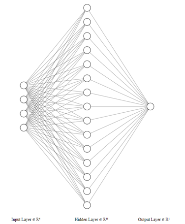
Measurement data is modeled using an artificial neural network (ANN) with input in the form of time, previous measurement data, and output in the form of current measurement data. The ANN scheme for modeling is shown in Figure 1. ANN consists of an input layer (leftmost) that receives data, hidden layers (middle) that process information using weights, biases, and activation functions, and an output layer (rightmost) that produces the final result. As a subset of machine learning, ANN is designed to recognize patterns and make predictions by learning from data through iterative training processes.
The ANN model is presented in a matrix form, with the number of nodes set to 15. The activation function in the hidden layer uses the sigmoid function while the output layer uses a linear function. The sigmoid activation function in the hidden layer and the linear activation function in the output layer were chosen because they are simple, commonly used, and fit the normalized input data range [16]. The mean square error (MSE) value was chosen at 0.01 as the standard for the iteration to finish. The learning algorithm used is Levenberg-Marquardt. The Levenberg-Marquardt algorithm is highly valued for its accuracy and is often applied in ANNs, but the probability of convergence at local extrema with errors approaching the global extrema is very low [17, 18]. The Adaptive Moment Estimation (ADAM) algorithm is an alternative algorithm that can be used for large datasets, deep models, and using modern frameworks such as TensorFlow/PyTorch. The general ANN equation is shown in Eq. (6).
Figure 1. ANN scheme
$\hat{y}={{f}_{o}}\left[ \sum\limits_{j=1}^{{{N}_{h}}}{{{w}_{o}}}{{f}_{h}}\left( \sum\limits_{i=1}^{{{N}_{x}}}{{{w}_{h}}}x+{{b}_{h}} \right)+{{b}_{o}} \right]$ (6)
wh is the hidden weight, x is the input data, bh is the input bias, fh is the activation function in the hidden layer, wo is the output weight, bo is the output bias, fo is the activation function in the output layer and yo is the model output. Nx is the number of inputs and Nh is the number of nodes.
2.5 Testing modeling
Model testing is carried out to see the difference in the difference between the model output and the actual measurement output. Testing is carried out using the mean square error (MSE) that measures the average squared difference between predicted and actual values. MSE is shown in Eq. (7) [19, 20].
$MSE=\frac{1}{{{N}_{y}}}\sum\limits_{i=1}^{{{N}_{y}}}{{{(y-\hat{y})}^{2}}}$ (7)
Ny is the amount of data from y, y is the measurement output, and $\hat{y}$ is the model output.
2.6 Design of anomaly detection
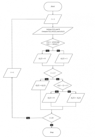
The measurement result is considered to be an anomaly (failure) when the measurement result exceeds the specified limits including the upper control limit (UCL) and lower control limit (LCL). The allowed error limit is five percent or 0.05. the UCL and LCL equations are shown in Eqs. (8) and (9). The anomaly detection algorithm flowchart is shown in Figure 2.
(a)
(b)
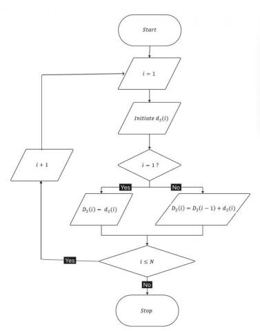
Figure 2. Flowchart (a) anomaly detection algorithm (b) calculation of the cumulative number of anomalies
$UCL(i)=y(i)+0.05y(i)$ (8)
$LCL(i)=y(i)+0.05y(i)$ (9)
The arrangement of the anomaly detection algorithm is as follows:
The arrangement of the cumulative anomaly calculation algorithm is as follows:
2.7 Design of reliability monitoring
The detected anomaly d2(i) is assumed to be a failure in the reliability calculation. Failures will be counted cumulatively, D2(i). Reliability calculations are carried out based on Benard's approximation which is shown in Eq. (10) [14].
$R(i)=1-\frac{{{D}_{2}}(i)-0.3}{{{N}_{{{D}_{2}}}}+0.4}$ (10)
R(i) is the current reliability in i, D2(i) is the cumulative failure and ND2 is the total number of failures.
3.1 Results of data acquisition and processing
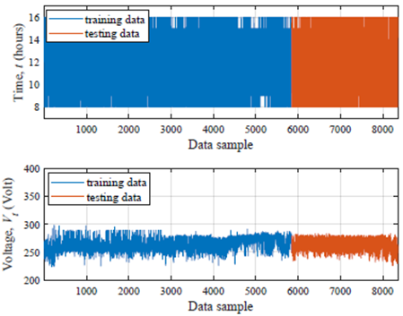
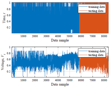
The results of the data division for training data and test data are shown in Figure 3 with a composition of 70:30. Figure 3 (a) is a graph of the training data and test data before the outliers and Figure 3 (b) is a graph of the training data and test data after the outliers. Outlier data is done to remove data that is outside the ideal data range. Data before the outlier range between 200.3 to 383 and after the outlier, data range between 223.6 to 298.2 with 51 data is removed. Outliers can have a significant influence on ANN modeling in real time monitoring. Figure 3 (a) shows that the voltage value fluctuates within the specified time range, with one instance where the value significantly spikes. Therefore, an outlier is performed for values that are outside the range so that Figure 3 (b) is obtained.
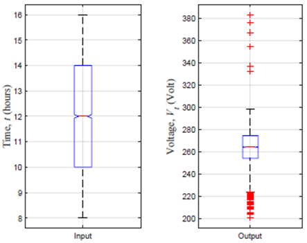
Figure 4 shows the box plots before and after the outliers for the time data and stress data. Box plots provide a visual representation of the quartiles, mean values, and outliers of the data set. Box plots also provide an overview of data that are outside the box plot or out of reach. MSEThe time variation is in the range of 10 to 14 hours and the voltage data variation is in the range of 254 volts to 274 volts. The result shows that in Figure 4 (a) there are still stress data that are outside the box plot, which means that the data is outside the range of the data, so these data must be removed. Figure 4 (b) shows that the data is already in the box plot area, which means that the data is within the measurement data range.
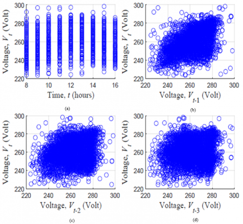
Figure 5 shows that there is a relationship between the voltage data from the current solar power plant, Vt with time t and the previous voltage data, Vt-k. Figure 5 (a) shows the relationship between the voltage data from the current solar power plant, Vt and the time, t correlation coefficient value of 0.2744 before removing outliers and 0.2725 after removing outliers. Figure 5 (b) shows the relationship between the current voltage data, Vt and the previous voltage data, Vt-k namely lag-1 (Vt-1), lag-2 (Vt-2), and lag-3 (Vt-3) respectively 0.6229, 0.3426, 0.1296 for before removing outliers and 0.6429, 0.3424, 0.1077 for after removing outliers. The value of the correlation coefficient can be seen in Table 1.
Table 1 shows that the largest correlation coefficient value is shown by the relationship between the current voltage data, Vt to previous data, Vt-1 for data after removing outliers, which is equal to 0.6429 which is classified as strong.
Figure 4. Box plot
Figure 5. Scatter plot (a)Vt to t; (b) Vt to Vt-1; (c) Vt to Vt-2; (d) Vt to Vt-3
Table 1. Correlation coefficient value
|
Input |
Output, Vt |
|
|
Before Removing The Outliers |
After Removing The Outliers |
|
|
t |
0.2744 |
0.2725 |
|
Vt-1 |
0.6229 |
0.6429 |
|
Vt-2 |
0.3426 |
0.3424 |
|
Vt-3 |
0.1296 |
0.1077 |
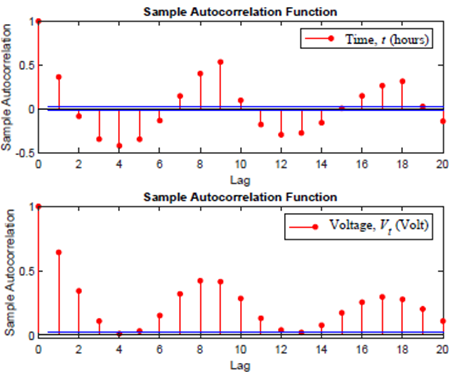
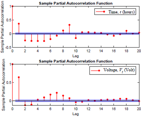
Figure 6 shows the ACF and PACF graphs from the training data and test data. Figure 6 (a) shows that there is no cut-off on the ACF graph but decreases following an exponential shape. Figure 6 (b) shows that there is almost a cut-off on the PACF graph. This shows that the time series method can be used in the design of reliability monitoring designs in real time.
Figure 7 shows a graph of normalized data from training data and test data. Normalization aims to make measurement data, namely time data and voltage data from the solar power plant, within the same range. Data normalization is typically performed within the range of 0 to 1 or -1 to 1. In this study, normalization is applied within the range of 0 to 1.
(a) ACF
(b) PACF
Figure 6. Graphic of correlation function
Figure 7. Graph of normalized data
3.2 Results of solar power plant modeling
The results of modeling solar power plant data obtained from ANN in matrix form are shown in Eq. (11) and Figure 8.
$w_k=\left[\begin{array}{cccc}4.333 & 4.324 & 0.364 & 8.210 \\ 0.689 & 9.413 & -0.499 & -4.797 \\ -4.681 & 6.177 & -6.012 & 4.071 \\ 9.591 & 1.243 & 4.183 & 3.582 \\ 6.088 & 9.722 & -0.242 & -6.759 \\ 6.814 & -3.898 & -5.133 & 1.857 \\ -3.940 & 9.085 & 4.484 & 0.384 \\ 1.298 & 8.228 & 5.075 & 5.790 \\ 5.729 & 6.322 & 6.601 & 5.250 \\ 12.880 & -4.161 & -1.979 & 3.278 \\ 5.969 & -0.774 & 5.474 & -7.249 \\ -7.998 & -3.909 & 3.114 & -2.091 \\ 0.945 & 8.737 & -5.064 & 2.118 \\ -6.252 & 10.753 & -0.610 & -0.103 \\ -1.991 & 7.002 & -4.411 & 5.020\end{array}\right] b_k=\left[\begin{array}{c}-16.787 \\ -8.876 \\ 1.613 \\ -11.669 \\ -5.241 \\ -2.085 \\ -5.535 \\ -9.546 \\ -11.842 \\ -2.292 \\ 0.758 \\ 2.971 \\ 1.358 \\ -4.342 \\ -10.364\end{array}\right]$ (11)
$\begin{aligned} & w_0=\left[\begin{array}{lllllllllllllll}-0.835 & -0.905 & 0.188 & -0.081 & 0.087 & -0.228 & 0.238 & -0.136 & 0.219 & -0.282 & -0.024 & -0.575 & -0.455 & -0.268 & 0.222\end{array}\right] \\ & b_0=\left[1.129 \right]\end{aligned}$
Figure 8. Comparison graph of the ANN model with measurement data output
Table 2. MSE value
|
Input |
MSE form Training Data |
MSE form Testing Data |
|
t, Vt-1 |
8.994×10⁻³ |
8.430×10⁻³ |
|
t, Vt-1, Vt-2 |
8.948×10⁻³ |
9.667×10⁻³ |
|
t, Vt-1, Vt-2, Vt-3 |
8.963×10⁻³ |
9.533×10⁻³ |
|
Vt-1, Vt-2, Vt-3 |
1.208×10⁻² |
1.408×10⁻² |
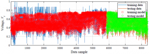
Figure 8 shows the results of matrix modeling using training data and test data. Figure 8 consists of a training data graph, namely the actual solar power plant power data and a test data graph, namely a graph of the modeling results with the matrix obtained. It can be seen that the resulting graph is close to the actual data graph. The MSE value from the results of a comparison of the training data graph and the test data can be seen in Table 2.
The smallest MSE value for reliability modeling using training data is 8.948×10⁻³ with the input variable time data, t and lag-1 voltage data, Vt-1. The MSE value in the training data for each variation of the input variable is not much different, which is in the range of 8.948×10⁻³ to 1.208×10⁻². The smallest MSE value for the model with test data is 8.948×10⁻³ with the input variable time data, lag-1, and lag-2 voltage data. MSE values in the test data are in the range of 8.994×10⁻³ to 1.408×10⁻². The ANN model is selected with t, Vt-1, Vt-2, Vt-3 as inputs. This is to accommodate all measurement values and to note that the MSE value is still less than 0.01.
3.3 Results of reliability modeling
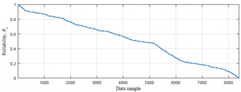
The results of reliability modeling for solar power plant are anomaly detection and reliability graph that are shown in Figure 9 and Figure 10.
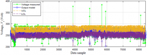
Figure 9 shows an anomaly detection graph, namely a graph that shows the results of comparing the model output with measurement output. The number of detected anomalies is 507 in 8402 data. Reliability calculations are carried out based on the anomalies that occur and are shown in Figure 9.
Figure 10 shows a graph of the reliability of a solar power plant. The reliability value of the solar power plant in the first year is 0.683 and will continue to decrease by 0.376 in the second year. To produce maximum reliability, it is necessary to optimize performance by operating according to Standard Operating Procedures (SOP). In addition, preventive maintenance needs to be done when the reliability reaches 0.55 with a maintenance interval of 21 months.
Figure 9. Graph of anomaly detection
Figure 10. Graph of reliability
Modeling of real time reliability monitoring system for solar power plants can be carried out using time series, past voltage data and time as input variables to predict future voltage data. The largest correlation coefficient value is the relationship between the voltage data from the current solar power plant to previous data for data after removing outliers, which is equal to 0.6429. The results of reliability modeling for the best predictive system are using input variables, time and voltage data with lag-1, lag-2, and lag-3. The resulting MSE value is 8,963×10-3 for training data and 9,533×10-3 for test data. The solar power plants reliability value was 0.683 in the first year and continued to decrease by 0.376 in the second year. Preventive maintenance needs to be done when reliability reaches 0.55 with a maintenance interval of 21 months. Implementing this real-time reliability monitoring system in existing solar power plants can optimize maintenance scheduling, reducing unexpected failures and operational downtime. This approach can lead to significant cost savings by extending the lifespan of system components and minimizing unnecessary maintenance expenses. Future research will develop a system for detecting or identifying types of errors in the machine using machine learning algorithms.
The authors gratefully acknowledge financial support from the Institut Teknologi Sepuluh Nopember for this work, under project scheme of the Departmental Fund Research Project 2024.
[1] Afif, F., Martin, A. (2022). Tinjauan potensi Dan Kebijakan energi surya di Indonesia. Jurnal Engine: Energi, Manufaktur, dan Material, 6(1): 43-52. https://doi.org/10.30588/jeemm.v6i1.997
[2] Rahman, Y.A., Pamuso, M., Fauzi, R., Siswanto, A. (2022). Performansi grid tie inverter dengan variasi pembebanan pada PV-On grid module trainer. ELKOMIKA: Jurnal Teknik Energi Elektrik, Teknik Telekomunikasi, & Teknik Elektronika, 10(2): 287. https://doi.org/10.26760/elkomika.v10i2.287
[3] Arsita, S.A., Saputro, G.E., Susanto, S. (2021). Perkembangan kebijakan energi nasional dan energi baru terbarukan Indonesia. Jurnal Syntax Transformation, 2(12): 1779-1788. https://doi.org/10.46799/jst.v2i12.473
[4] Silaban, S., Sitompul, P. (2023). Instalasi pembangkit listrik tenaga surya kapasitas 450 watt. Sinergi Polmed: Jurnal Ilmiah Teknik Mesin, 4(1): 41-48. https://doi.org/10.51510/sinergipolmed.v4i1.1011
[5] Nur’Aini, E., Budiarto, R., Setiawan, B., Ma'arif, A. (2021). Reliability analysis and maintainability for the design of grid and hybrid solar power plant systems in Wonogiri Regency. ELKHA: Jurnal Teknik Elektro, 13(1): 77-83.
[6] Gangwar, L., Singh, S. (2024). Reliability analysis of different capacities solar PV power plant. IOSR Journal of Electrical and Electronics Engineerin, 19(3): 1-15. https://doi.org/10.9790/0853-1903010115
[7] Raghuwanshi, S.S., Arya, R. (2020). Reliability evaluation of stand-alone hybrid photovoltaic energy system for rural healthcare centre. Sustainable Energy Technologies and Assessments, 37: 100624. https://doi.org/10.1016/j.seta.2019.100624
[8] Romeu, J.L. (2003). Practical reliability engineering. Technometrics, 45(2): 173. https://doi.org/10.1198/tech.2003.s133
[9] Causia Aguisti, F., Musyafa, A., Khamim Asy'ari, M. (2020). Analysis of RAM (Reliability, Availability, Maintainability) Production of Electric Voltage from 48 v PV (Photovoltaic) at Pantai Baru Pandansimo, Indonesia. E3S Web of Conferences, 190: 00010. https://doi.org/10.1051/e3sconf/202019000010
[10] Fitrianingtyas, P., Asy’ari, M.K., Elyawati, N., Musyafa, A. (2024). Reliability, maintainability and availability analysis of solar power plant in Pantai Baru using voltage measurement data. E3S Web of Conferences, 479: 05001. https://doi.org/10.1051/e3sconf/202447905001
[11] Liu, Y. (2021). Reliability analysis of photovoltaic module based on measured data. In IOP Conference Series: Earth and Environmental Science. IOP Publishing, 793(1): 012019. https://doi.org/10.1088/1755-1315/793/1/012019
[12] Sayed, A., El-Shimy, M., El-Metwally, M., Elshahed, M. (2019). Reliability, availability and maintainability analysis for grid-Connected solar photovoltaic systems. Energies, 12(7): 1213. https://doi.org/10.3390/en12071213
[13] Ervintyana, L., Widjaja, A., Liliawati, S.L. (2023). Analisis deret waktu dari produk yang terjual menggunakan beberapa teknik populer. Jurnal Teknik Informatika dan Sistem Informasi, 9(1): 110-126. https://doi.org/10.28932/jutisi.v9i1.5933
[14] Ebeling, C.E. (2019). An Introduction to Reliability and Maintainability Engineering. Waveland Press.
[15] Heteroskedasticity, A.C. (2018). Implemetasi model autoregressive (AR) dan autoregressive conditional heteroskedasticity (ARCH) untuk memprediksi harga emas. Indonesian Journal on Computing, 3(2): 29-44. https://doi.org/10.21108/indojc.2018.3.2.225
[16] Goyal, M., Goyal, R., Lall, B. (2019). Learning activation functions: A new paradigm for understanding neural networks. arXiv preprint arXiv:1906.09529. https://doi.org/10.48550/arXiv.1906.09529
[17] Mikhaylov, A., Tarakanov, S. (2020). Development of levenberg-Marquardt theoretical approach for electric networks. Journal of Physics: Conference Series, 1515(5): 052006. https://doi.org/10.1088/1742-6596/1515/5/052006
[18] Giap, Q.H., Nguyen, D.L., Nguyen, T.T.Q., Tran, T.M.D. (2022). Applying neural network and levenberg-Marquardt algorithm for load forecasting in IA-Grai district, gia lai province. Tạp chí Khoa học và Công nghệ-Đại học Đà Nẵng, 20(6): 13-18. https://doi.org/10.31130/ud-jst.2022.240ict
[19] Asy’ari, M.K., Noriyati, R.D., Indriawati, K. (2019). Soft sensor design of solar irradiance using multiple linear regression. In 2019 International Seminar on Intelligent Technology and Its Applications (ISITIA), Surabaya, Indonesia, pp. 56-60. https://doi.org/10.1109/ISITIA.2019.8937150
[20] Mukromin, R.I., Asy'ari, M.K. (2020). Prediksi daya panel surya kapasitas 50 wp menggunakan model regresi linier majemuk. Jurnal Teknologi Bahan dan Barang Teknik, 10(2): 58-65. https://doi.org/10.37209/jtbbt.v10i2.166