Jose Manuel Palomino Ojeda*![]() | Lenin Quiñones Huatangari
| Lenin Quiñones Huatangari![]() | Jeiden Revilla Arce
| Jeiden Revilla Arce![]() | Nilthon Arce Fernández
| Nilthon Arce Fernández![]() | Marcos Antonio Gonzales Santisteban
| Marcos Antonio Gonzales Santisteban![]() | Marco Antonio Martínez Serrano
| Marco Antonio Martínez Serrano![]()
© 2024 The authors. This article is published by IIETA and is licensed under the CC BY 4.0 license (http://creativecommons.org/licenses/by/4.0/).
OPEN ACCESS
In Peru, confined masonry houses are self-built, which makes it crucial to determine their seismic vulnerability. The objective of the research was to estimate the seismic vulnerability of confined masonry dwellings in the Pueblo Libre-Jaén sector using assembly algorithms. A database was constructed with data obtained from the National Institute of Civil Defense (INDECI), scientific articles, and theses. Subsequently, the data set was divided into a training set (80%) and a validation set (20%), employing the stacking method with five combinations CB_1, CB_2, CB_3, CB_4, and CB_5. The basic algorithms Gradient-Boosting, Random-Forest, Extra-Tree, and Decision-Tree were utilized as the base algorithms, with the final estimator being the Random Forest Meta-Learner. The models were trained and validated in Python, achieving accuracies of 94.95, 95.48, 95.39, and 95.66 for the base models and 95.62, 95.23, 95.76, 95.90, and 94.80% for the ensemble models. The most accurate models were the simple Gradient Boosting (95.66%) and the assembled models CB_3 (95.76%) and CB_4 (95.90%). The CB_4 model, which is composed of the Decision Tree and Gradient Boosting algorithms, was applied to the Pueblo Libre sector and yielded a reliability estimate of greater than 95% for the seismic vulnerability of confined masonry. This estimate was classified as high (1.48%), moderate (32.85%), and low (65.67%). It is anticipated that the model implemented will enable engineers and authorities to implement mitigation measures to reinforce housing in the event of a seismic event.
automation, ensembled algorithms, Gradient Boosting, masonry housing, seismic vulnerability, random forest
Seismic vulnerability is the susceptibility of a region, structure, or population to damage or loss from an earthquake [1]. It includes factors such as building quality, soil type, geographic location, seismic response capacity [2], type of material, structural system, workmanship [3], structural fragility, population density, and disaster response capability are pivotal factors that influence a community's resilience in the face of seismic events. These constituents permit nations susceptible to natural disasters to quantify fundamental aspects of vulnerability and delineate their capacities for national risk management [4, 5].
Confined masonry dwellings are widely used due to their low cost compared to other structural systems [6]. They are subjected to seismic movements of varying intensities caused by the movement of tectonic plates, resulting in human, economic, and material losses [7].
In Peru, most masonry constructions are self-built and do not adhere to the technical masonry standard (E.070) or the seismic design standard (E.030). Instead, they are based on the advice of a mason or master mason with empirical knowledge, resulting in structures that are vulnerable to seismic events. As a result, these houses do not ensure proper structural behavior or the safety of their inhabitants [8]. Several buildings in Arequipa (16 incidents), Ica (12 incidents), Tacna (9 incidents), and Ucayali (8 incidents) have suffered damage and structural deterioration due to frequent earthquakes with magnitudes greater than 5.0 on the Richter scale. This damage has been irreparable and has caused the collapse of the buildings [1]. Seismic events have occurred frequently, causing damage to masonry houses, such as cracks in walls, columns, and beams, leaving them vulnerable to future seismic events [9].
Determining seismic vulnerability involves both qualitative and quantitative methods, each requiring different approaches and data depending on factors such as the country [4], time, costs, and resources [10]. This presents a challenge for researchers and professionals involved in assessing and managing seismic vulnerability, as gaps in the literature must be identified. Ortega et al. [10], evaluated the seismic vulnerability of vernacular buildings using the SVIVA methodology; however, their research did not include the analysis of masonry dwellings. Firmansyah et al. [2] highlight the paucity of research on the impact of limited building data on the accuracy of large-scale vulnerability assessment models in low- and middle-income countries. Bektaş and Kegyes-Brassai [11] note that some studies rely on data collected from a single geographic location, which restricts the applicability of methods developed at a regional or global level. This generates the need for further improvement of seismic vulnerability assessment methods to achieve greater accuracy and applicability in different contexts.
Ensemble methods are effective strategies for improving the generalization and robustness of predictive models. They improve model predictive performance by individually training several models and integrating their predictions. This is achieved by integrating predictions from multiple base estimators, which are constructed using a specific learning algorithm or a combination of several algorithms [12].
The research proposes a new method for classifying large-scale seismic vulnerability using ensemble algorithms. It addresses gaps in the literature by extracting patterns from large databases to accurately identify factors that influence vulnerability to seismic events. Furthermore, this methodology aids in the creation of sturdy and dependable predictive models that can adjust to various forms of geographic and structural data, among others.
The research aimed to estimate the seismic vulnerability of confined masonry housing in the Pueblo Libre sector. Assembly algorithms were employed to estimate the level of vulnerability, categorizing it as low, medium, or high, as well as identifying potential damage scenarios that could ensue in the event of a seismic event.
Researchers have employed various techniques to assess seismic vulnerability. Ortega et al. [10] developed a vulnerability index formula, SVIVA, to assess the seismic susceptibility of vernacular dwellings. To this end, they conducted a comprehensive analysis of key parameters and assigned weights to them through statistical analysis and expert judgment. They then proceeded to analyze the seismic behavior of the buildings through parametric numerical simulations using finite element models to study the influence of the selected parameters.
Izquierdo et al. [1] analyzed seismic vulnerability in the Pisco region of Peru by integrating machine learning and hierarchical analysis methods to assess seismic risk. The methodology used Random Forest to assess seismic hazard and AHP for vulnerability, focusing on social and physical factors.
Rojas et al. [13] evaluated the structural integrity of blocks B3 and B4 at the Humberto Molina Hospital in Zaruma, Ecuador, using the international code ASCE/SEI 41-13. The evaluation aimed to identify structural deficiencies and propose rehabilitation alternatives. The methodology involved collecting basic information, conducting field inspections, evaluating the structure, and proposing rehabilitation alternatives. The study revealed overall inadequacies in the hospital facilities, and recommendations for rehabilitation were provided based on national and international standards.
Firmansyah et al. [2] conducted vulnerability assessments at a regional scale to identify building typology through an objective labeling process using a decision tree. In the initial phase, a decision tree was constructed to classify building typology. This was trailed by the growth of a machine learning model utilizing a convolutional neural network (CNN) trained on labeled datasets in the subsequent phase. Finally, in the third phase, the potential utility of the CNN model for assessing city vulnerability was examined. The study found that the CNN model enhanced the identification of building typology, enabling the estimation of the city's structural vulnerability.
Bektaş and Kegyes-Brassai [11] developed a seismic vulnerability assessment (SVR) method that demonstrated higher accuracy than conventional methods based on neural networks. The SVR method was compared to conventional methods and neural networks, and it showed higher applicability and accuracy. The results indicated that the SVR method achieved an accuracy of 68%, significantly higher than that of conventional methods, which have rates lower than 30%. The importance of adopting a new framework for developing SVR methods that incorporate artificial intelligence algorithms, machine learning, such as fuzzy logic, and neural networks, to construct models based on multiple data is emphasized.
Sauti et al. [14] developed an index for seismic hazard exposure in the Sabah Municipal District by identifying and constructing exposure vulnerability indicators. The methodology included multivariate data normalization, calculation of weights of indicator variables, and map overlay to assess seismic risk. The results showed that combining spatial data and statistical analysis is a feasible approach to assessing vulnerability to natural disasters.
López-Almansa and Montaña [15] conducted an investigation into the seismic vulnerability of mid-rise steel structures in Bogotá, Colombia. The study involved numerical and seismic performance evaluation analyses of eighteen representative prototype buildings with varied earthquake-resistant systems. The seismic responses of these buildings were compared.
Najar et al. [16] developed a land use planning framework based on seismic micro zonation to reduce seismic vulnerability and promote resilience to natural disasters. They performed seismic hazard assessment, soil response analysis, liquefaction analysis, and seismic micro zonation using technologies such as geographic information systems (GIS) and geospatial modeling. The study indicates that incorporating seismic zoning regulations into land use planning can enhance a city's resilience to seismic disasters by identifying high-risk areas and proposing mitigation measures.
Talledo et al. [17] conducted a study to assess the efficacy of reinforced concrete technology for combined seismic and thermal strengthening interventions in existing buildings. The study demonstrated the suitability of the technology in seismic risk class assessment. The methodology included numerical analyses to evaluate the proposed technology in an existing reinforced concrete building. The analyses employed synthetic measures, including Expected Annual Loss and Life Safety Index. The findings of the study demonstrated that the implementation of reinforced concrete technology led to an enhancement of the seismic risk rating of the evaluated building.
Lin et al. [18] enhanced the multi-hazard resilience of multi-story reinforced concrete structures through the implementation of a novel precast portal frame system, designated as the multi-hazard resistant precast concrete (MHRPC) system. The researchers employed a methodology that included cyclic seismic testing and progressive collapse testing on three types of portal frames: conventional, progressive collapse design, and the MHRPC system. The findings indicated that the progressive collapse design exerted a pronounced influence on the seismic behavior of the structures.
Huang et al. [19] examined the seismic performance of staggered stringer truss systems through experimental and numerical analysis, focusing on different failure modes. The methodology included the design and testing of two truss specimens, which demonstrated that the specimen designed for chord failure exhibited superior seismic performance. The experimental results demonstrated that the specimens ST1 and ST2 exhibited different behaviors under load. Specimen ST1 exhibited higher lateral stiffness and energy dissipation capacity compared to ST2.
Sadeghi et al. [20] evaluated and compared the seismic performance of buildings constructed using industrial and conventional techniques in Iran. The researchers employed nonlinear incremental dynamic analysis to assess the seismic behavior of three structural systems. The findings indicated that reinforced concrete shear walls exhibited more reliable collapse fragility curves and outperformed typical eccentrically braced portal frames. Moreover, modern buildings constructed with industrial methods exhibited a lower seismic risk and superior overall performance compared to traditional construction techniques.
Several authors employ a variety of models to assess the seismic vulnerability of constructions. These include mathematical, statistical, vulnerability index, machine learning, deep learning, progressive collapse design, numerical analysis, and seismic performance assessment models; land use planning based on seismic micro zoning; nonlinear finite element models; and models based on international codes (see Table 1). There is a dearth of research investigating the utilization of ensemble algorithms to assess seismic vulnerability in confined masonry dwellings.
Table 1. Models for the estimation of seismic vulnerability of buildings
|
Autor |
Parameters |
Method |
Application |
|
Ortega et al. [10] |
Wall slenderness, Roof thrust, Type of material, Horizontal diaphragms, Maximum wall span, Wall openings, Number of floors, Previous structural damage, In-plane index and Wall-to-wall connections |
Vulnerability index |
Seismic evaluation of vernacular buildings |
|
Izquierdo et al. [1] |
Soil type, DEM, Bearing capacity, Slope, Land use |
Machine learning (Random Forest) and hierarchical analysis |
Seismic risk assessment |
|
Rojas et al. [13] |
Architectural configuration, material condition, and structural system, |
International Code ASCE/SEI 41-13 |
Structural evaluation of blocks B3 and B4 of the Humberto Molina Hospital in Zaruma, Ecuador |
|
Firmansyah et al. [2] |
Confined Masonry, RC Infilled Masonry, Timber Structure, and Unconfined Masonry |
Convolutional Neural Networks (CNN) |
Vulnerability assessment at the regional scale |
|
Bektaş and Kegyes-Brassai [11] |
Age of the structure, building height, number of floors, ground floor configuration, roof design, building positioning, plinth area, distance from the seismic source, foundation type, other floor constructions, plan irregularities, land surface conditions, risk of liquefaction, fundamental period, and spectral acceleration |
Neural Networks (ANN) |
Estimation of seismic vulnerability |
|
Sauti et al. [14] |
Age structure, Gender, Population density, Household density, Household residence density, and Building (residential) density |
Multivariate statistical analysis |
Generation of a seismic risk exposure map in the Sabah municipal district |
|
López et al. [15] |
Direction, Vertical distribution, Length, Earthquake-resisting system, and Number of floors |
Numerical and seismic performance evaluation analysis |
Seismic vulnerability of medium-rise steel buildings in Bogota, Colombia |
|
Najar et al. [16] |
The intensity of ground motion, subsurface characteristics, liquefaction potential, and amplification of seismic waves |
Land use planning based on seismic microzonation |
Reducing seismic vulnerability and promoting resilience to natural disasters |
|
Talledo et al. [17] |
RC-framed skin with external plaster and RC buildings retrofitted with bare RC-framed skin |
Numerical analysis |
Evaluation of seismic risk class |
|
Lin et al. [18] |
Self-centering/high-strength prestressed tendons, resistance to progressive collapse forces, and the behavior of beam-column joints |
Progressive collapse design |
Precast concrete structural system engineered to withstand multiple hazards, addressing both seismic and structural requirements |
|
Huang et al. [19] |
Hysteresis loop, structural rigidity, dissipated energy, and ductility factor |
Capacity design method |
Evaluate the seismic effectiveness of the staggered truss system across diverse failure mechanisms |
|
Sadeghi et al. [20] |
Modular design, execution, integrated Management, executor experiences, desirability and comfort |
Evaluation using nonlinear finite element models |
Contrasts the seismic performance of structures erected through industrial construction techniques with conventional Iranian building methods |
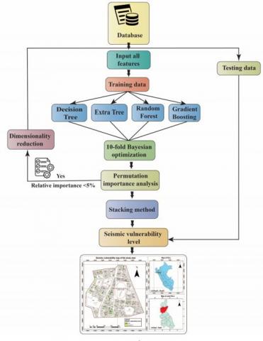
The study implemented assembly algorithms to determine the seismic vulnerability of masonry houses. A database of 3760 masonry houses was compiled from various repositories in Peru. The variables were entered and the base models were trained, including Decision-Tree, Extra-Trees, Random-Forest, and Gradient-Boosting, using a 10-fold cross-validation with the Bayesian method. The process involved analyzing the relevance of each variable about seismic vulnerability. If the dimensionality was less than 5%, the variables were reduced from eleven to seven. Following this, a training (80%) and validation (20%) data set were created. Finally, five ensemble models were developed using the Stacking method, with the Random-Forest meta-classifier. This method integrates the forecasts from multiple base classifiers to enhance the final prediction accuracy. Once the model had been validated using the validation dataset, it was applied to assess the seismic vulnerability of confined masonry dwellings in the Pueblo Libre sector of Jaen, Cajamarca, Peru (see Figure 1).
3.1 Seismic vulnerability
The susceptibility of a building or structure to damage or collapse due to the action of an earthquake. This can be reduced by reinforcement or protection measures to better resist seismic forces [21]. In a building, this is contingent upon the absence of attributes that impact the structural components. These deficiencies can be attributed to a number of factors, including the effects of aging, inadequate maintenance, outdated design, material properties, construction site conditions, and natural phenomena [22].
There are different evaluation methods, with the vulnerability index being the most widely used to determine the seismic vulnerability of masonry buildings [23]. The Benedetti-Petrini vulnerability scale for masonry buildings was employed as a foundation for this study. The parameters were derived by applying a weighted sum of numerical values representing the "seismic quality" of each structural and nonstructural factor that affects the seismic behavior of masonry structures. Each parameter was assigned, during the technical visits (inspections), one of the four classes A, B, C, and D. The "A" rating is optimal with a numerical value Ki=0, while "D" is the most unfavorable with a numerical value Ki=45 [24], as shown in Tables 2 and 3. For example, if parameter number four "Building location and foundation" corresponds to a seismically unsafe configuration, it is assigned a rating of "D" and a numerical value of K4=45. Table 2 illustrates the 11 structural parameters utilized by Peruvian Standard E-0.70 (confined masonry), with the parameters assigned the attributes A, B, C, and D based on their compliance with the aforementioned structural parameters.
Figure 1. Research flowchart
Table 2. Structural parameters for seismic vulnerability assessment
|
Parameter |
Symbol |
Description |
|
Type and organization of the resistant system |
TO |
A: Masonry buildings complying with the E 070 standard B: Buildings that do not comply with at least one requirement of E 070 C: Buildings with beams and columns that are only partially confining D: Buildings without confinement beams or columns or self-construction |
|
Resistant system quality |
RS |
A: The building's resistant system has the following three characteristics:
B: The resistant system does not have one of the characteristics of class A C: The resilient system does not exhibit two of the characteristics of Class A D: The resistant system does not have any of the characteristics of class A |
|
Conventional resistance |
CR |
A: RC < 0.50 B: 0.50 ≤ RC < 1.00 C: 1.00 ≤ RC < 1.50 D: 1.50 ≤ RC |
|
Position of the building and foundation |
PB |
A: Building founded on rigid soil and by standard E - 070 B: Building founded on intermediate and flexible soil, according to standard E - 070 C: Building founded on intermediate and flexible soil, according to standard E - 070 D: Building founded without an approved project or technical advice |
|
Horizontal diaphragms |
HD |
A: Diaphragm buildings that meet the following conditions
B: Building that does not comply with one of the Class A conditions C: Building that does not comply with two of the Class A conditions D: Building that does not comply with any of the conditions of Class A |
|
Plant configuration |
PC |
A: IRP ≤ 0.10 B: 0.10 < IRP ≤ 0.50 C: 0.50 < IRP ≤ 1.00 D: IRP > 1.00 |
|
Configuration in elevation |
CE |
A: Building with: ± ΔA/A ≤ 10% B: Building with: 10% < ± ΔA/A ≤ 20% C: Building with: 20% < ± ΔA/A ≤ 50% D: Building with: ± ΔA/A ≥ 50%; Presents irregularities of soft floor |
|
Maximum distance between walls |
MD |
A: Building with L/S < 15 B: Building with 15 ≤ L/S ≤ 18 C: Building with 18 ≤ L/S ≤ 25 D: Building with L/S ≥ 25 |
|
Type of cover |
TC |
A: Stable cover duly fastened to the walls with appropriate connections B: Unstable cover made of light material and in good condition C: Unstable cover made of light material and in poor condition D: Unstable deck in poor and uneven conditions |
|
Non-structural elements |
NE |
A: Building that does not contain poorly connected non-structural elements B: Building with balconies and parapets well connected to the resistant system C: Building with balconies and parapets poorly connected to the resistant system D: Building that has water tanks or any other type of element |
|
State of conservation |
SC |
A: Walls in perfect condition and without visible cracks B: Walls in good condition, with small cracks, less than two millimeters C: Building without cracks, but in a poor state of repair D: Walls with strong deterioration in their components |
After evaluating each parameter, a weighted sum was performed using the weight factors to obtain the final vulnerability index using Eq. (1) [25, 26]:
$I v=\sum_{i=1}^{11} k i * W i$ (1)
where:
$I v$: Benedetti-Petrini vulnerability index.
$k i$: Numerical value of the vulnerability index of Benedetti-Petrini.
$W i$: Weight coefficient of the Benedetti-Petrini vulnerability index.
Table 3. Benedetti-Petrini vulnerability scale
|
Parameters |
Ki Class |
Factor |
|||
|
A |
B |
C |
D |
Wi |
|
|
CR |
0 |
5 |
25 |
45 |
1.50 |
|
TO |
0 |
5 |
20 |
45 |
1.00 |
|
HD |
0 |
5 |
15 |
45 |
1.00 |
|
CE |
0 |
5 |
25 |
45 |
1.00 |
|
TC |
0 |
15 |
25 |
45 |
1.00 |
|
SC |
0 |
5 |
25 |
45 |
1.00 |
|
PB |
0 |
5 |
25 |
45 |
0.75 |
|
RS |
0 |
5 |
25 |
45 |
0.25 |
|
MD |
0 |
5 |
25 |
45 |
0.25 |
|
NE |
0 |
0 |
25 |
45 |
0.25 |
After the evaluation of the Vulnerability Index ($I v$) corresponding to each confined masonry structure, whose values range from 0 to 382.5 according to the established methodology, the process of normalizing the Normalized Vulnerability Index ($I v n$) to a scale of 0 to 100 was initiated, see Eq. (2).
$I v n=\frac{I v * 100}{382.5}$ (2)
where:
$I v n$ = Normalized Vulnerability Index.
$I v $ = Vulnerability index.
After finding the normalized vulnerability index, which ranges from 0 to 100, it was classified according to the vulnerability ranges in Table 4.
Table 4. Vulnerability index ranges
|
Vulnerability Assessment Scale |
|
|
0 < Ivn < 20 |
Low |
|
20 ≤ Ivn < 40 |
Moderate |
|
Ivn ≥ 40 |
High |
3.2 Algorithms
3.2.1 Decision tree
It is a structure in which data is divided according to a criterion (test). Each node of the tree represents a distinct test on a specific attribute. Each branch represents the outcome of the test, while the leaves of the node indicate the classes or distributions of classes. Each data instance has several attributes, one of which (the target or class attribute) indicates the class to which each instance belongs. The ID3, C4.5, and J4.8 algorithms are some examples of commonly used decision trees. They also offer the benefit of generating comprehensible models with satisfactory accuracy across various application domains. Information gain is the difference in entropy before and after a change. Entropy represents the expected value of information, defined as -log2(xi) where xi is the frequency of the classification label in the sample set S recorded as p(xi) [27].
3.2.2 Extra tree
The algorithm, integrated within the Python sci-kit-learn module, is distinguished by its user-friendly interface, which requires minimal adjustment of meta-parameters, and its demonstrated computational efficiency. The algorithm is parameterized by three key aspects during the training phase. The first parameter determines the maximum number of features (K) that are considered for node splitting during the construction of decision trees. The second parameter specifies the minimum sample size required for node division. Finally, the third parameter indicates the number of trees (ntrees) included in the ensemble. Furthermore, the algorithm demonstrates a reduced susceptibility to overfitting in comparison to alternative techniques such as neural networks or individual decision trees. This reduced susceptibility to overfitting arises from the tendency of the algorithm to avoid capturing idiosyncratic features specific to the training data, including random noise, which may not generalize well to other samples from the same distribution. Conversely, ensemble learning methods are generally more resilient against this phenomenon. It is noteworthy that the Extra-Trees algorithm was specifically designed to address this concern [28].
3.2.3 Random forest
The algorithm is an integral component of the learning process. It employs multiple randomized decision trees, integrating their predictions through the averaging process. The algorithm is comprised of two principal phases: construction and prediction. In the construction phase, a number of decision trees are generated using different training sets. The objective is to create an accurate model while minimizing the risk of overfitting. In the subsequent prediction phase, the final result is obtained by averaging the predictions of each tree. The efficacy of the algorithm is gauged by a multitude of metrics, including the resilience of the classifier parameters to perturbation, the capacity to withstand noise, and fluctuations in the size of the training set [29]. Table 5 provides a detailed account of the algorithm, as presented by Sagi et al. [12], including a comprehensive overview of its inputs and outputs.
Table 5. Structure of the random forest
|
Random Forest |
|
Input: $I D T$ (a decision tree inductor), T (The iteration count), S (training set), $\mu$ (the size of the subsample.), N (the count of attributes utilized in each node). Output: $M_t: \forall=1, \ldots, T$ for each in $1, \ldots, T$A do $S_t \leftarrow$ Sample $\mu$ instances from $S$ with replacement, Build a classifier $M_t$ using IDT (N) on $S_t$ $t++$ end |
3.2.4 Gradient Boosting
The presented method is an ensemble learning approach that constructs a predictive model through the iterative incorporation of sequentially adjusted weak learners, as demonstrated in Eqs. (3)-(5). he general problem is to learn a functional mapping $y=F(X ; \beta)$ from data $\left\{x_i, y_i\right\}_{i=1}^n$ where is the set of parameters of F such that some cost function is minimized. Boosting assumes $F(x)$ follows an “additive” expansion form $F(x)=\sum_{m=0}^M p_m f\left(x, \tau_m\right)$, where, $f$ is called the weak or base learner with a weight $\rho$ and a parameter set $\mathcal{\tau}$ accordingly, $\left\{p_m, \tau_m\right\}_{m=1}^M$ compose the whole parameter set $\beta$. Gradient Boosting approximates with two steps. First, it fits $f\left(x ; \tau_m\right)$ by:
$\tau_m=\arg \min \sum_{i=1}^n\left(g_{i m}-f\left(x_i, \tau\right)\right)^2$ (3)
where,
$g_{i m}=\left[\frac{\partial \Phi\left(y_i, F\left(x_i\right)\right)}{\partial F\left(x_i\right)}\right]_{F(x)=F_{m-1(x)}}$ (4)
Second, it learns $\rho$ by:
$p_m=\arg \min \sum_{i=1}^n \Phi\left(y, F_{m-1}\left(x_i\right)+p f\left(x_i ; \tau_m\right)\right)$ (5)
Then, it updates $F_m(x)=F_{m-1}(x)+p_m f\left(x ; \tau_m\right)$ [30]. In practice, however, shrinkage is often introduced to control overfitting, and the update becomes $F_m(x)=F_{m-1}(x)+v p_m f\left(x ; \tau_m\right)$, where, $0<v \leq 1$. If the weak learner is the regression tree, the complexity of $f(x)$. The GBM's performance is influenced by tree depth and the minimum number of samples at end nodes. In addition to choosing appropriate parameters for shrinkage and tree structure, subsampling can further improve the model's performance [31]. The performance of the GBM can be improved by subsampling, which involves fitting each base learner to a random subset of the training data. This can help increase the diversity among trees and improve the predictive ability of the overall model.
3.3 Data matrix
A database was created using information from the National Institute of Civil Defense (INDECI), scientific articles, and theses related to the seismic vulnerability of masonry dwellings. The data was collected from various academic repositories in Peru between 2017 and 2023 using data collection sheets for 3827 masonry dwellings. The variables considered in this study include the building location and foundation, type and organization of the resistant system, quality of the resistant system, horizontal diaphragms, plan configuration, elevation configuration, maximum distance between walls, type of roof, nonstructural elements, state of preservation, conventional resistance, and seismic vulnerability. These variables are based on the Benedetti Petrini method [10, 32]. Table 6 displays the description, type, and range of variables A, B, C, and D, while Figure 2 shows their respective frequencies. Additionally, Table 7 presents the descriptive statistical analysis of the variables, including unique values and the frequency of the maximum class.
Table 6. Description, classification, and scope of the 12 variables collected
|
Variable |
Description |
Type |
Range |
|
Type and organization of the resistant system |
Rate the degree of organization of the vertical elements. |
Ordinal |
A, B, C, D |
|
Resistant system quality |
It characterizes the type of masonry commonly utilized, contingent upon the material's type and homogeneity |
Ordinal |
A, B, C, D |
|
Conventional resistance |
It rates the reliability of the resistance that the building can withstand against horizontal loads. |
Ordinal |
A, B, C, D |
|
Position of the building and foundation |
It delineates the impact of soil and foundation characteristics on seismic behavior |
Ordinal |
A, B, C, D |
|
Horizontal diaphragms |
Qualifies the connection of the vertical resisting system at the transition of vertical loads. |
Ordinal |
A, B, C, D |
|
Plant configuration |
It qualifies the plant shape of the building |
Ordinal |
A, B, C, D |
|
Configuration in elevation |
It qualifies the elevation shape of the building |
Ordinal |
A, B, C, D |
|
Maximum distance between walls |
It qualifies excessive spacing between transversely located walls. |
Ordinal |
A, B, C, D |
|
Type of cover |
It specifies the typology and assigns a determined weight to the roof structure of a building |
Ordinal |
A, B, C, D |
|
Non-structural elements |
It qualifies the non-structural elements present in a building that can cause damage |
Ordinal |
A, B, C, D |
|
State of conservation |
It qualifies the presence of internal flaws in the structure, produced by failures in the construction process |
Ordinal |
A, B, C, D |
|
Seismic vulnerability |
Estimates the vulnerability index inherent in the buildings |
Ordinal |
High, Moderate, Low |
Table 7. Descriptive statistics of the variables
|
Variables |
Unique |
Top |
Freq |
|
Conventional resistance |
4 |
B |
1857 |
|
Type and organization of the resistant system |
4 |
B |
1871 |
|
Resistant system quality |
4 |
C |
2429 |
|
Horizontal diaphragms |
4 |
A |
1720 |
|
Positioning of the building and foundation |
4 |
C |
2319 |
|
Maximum distance between walls |
4 |
C |
2434 |
|
Plant configuration |
4 |
A |
2952 |
|
Configuration in elevation |
4 |
A |
3071 |
|
State of conservation |
4 |
B |
2002 |
|
Type of cover |
4 |
A |
2415 |
|
Non-structural elements |
4 |
A |
2171 |
|
Seismic vulnerability |
3 |
Moderate |
1961 |
Figure 2. Frequencies of each variable of the database
3.4 Study area
The masonry houses in Jaen, which are constructed in a traditional manner using handmade materials and without the guidance of a professional in the construction process (see Figure 3), were selected to apply the algorithm that had been trained and validated in the research. For this reason, the houses of the Pueblo Libre sector were studied, taking into account the seismic risk of the city of Jaén, which is located in seismic zone two according to the E.030 standard. The sector is situated in the province of Jaén, department of Cajamarca, Peru, at the following geographical coordinates: 5°42'12.06"S, 78°48'25.61"W (see Figure 4).
Figure 3. Confined masonry dwellings Jaen, Peru
3.5 Data processing
3.5.1 Selection of variables
Ensemble algorithms were used to estimate the seismic vulnerability of masonry houses in the Pueblo Libre sector of Jaen. A target dataset was selected for the discovery process. The Python programming language was used in this stage to select attributes based on the 'Random Forest Feature Importance' algorithm. This algorithm assigns weights to each variable based on its relevance to the output variable, which in this case is seismic vulnerability. After classifying the attributes, we reduced the dimensionality of the variables since their relative importance is less than 5%, resulting in a value of 1.8%. Consequently, we employed seven input variables that yielded the most information regarding the output variable, seismic vulnerability.
Figure 4. Map of the study area
3.5.2 Data standardization
The 'Label Encoding' technique was used to standardize variables in the dataset. This technique involves iterating over each column in the categorical dataset and creating a LabelEncoder object. The LabelEncoder class, which is part of the scikit-learn library, is used to transform categorical variables into numeric variables by assigning them a unique numeric value.
3.5.3 Pre-processing
To enhance data quality, we conducted a thorough data cleaning process to rectify anomalous data. Our cleaning procedures specifically targeted two main issues: missing values in certain records and duplicate data entries. The Python programming language, in conjunction with the Jupyter interface, was employed to achieve this objective. The pandas and NumPy data analysis libraries, which are both highly sophisticated and powerful, were leveraged to accomplish this task.
3.6 Ensemble combination
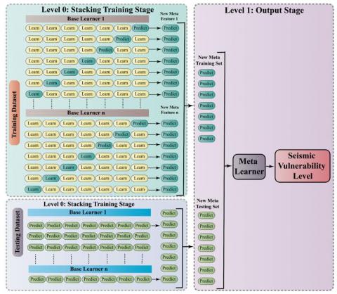
The study employed a hierarchical algorithm ensemble (SG) approach to enhance the performance of the model. This approach comprises two stages of learning. In the initial stage, a combination of machine learning algorithms, including CART, MARS, and Lasso, among others, is employed to generate a set of metadata from the original training set [33]. In the second stage, the meta-learner is employed to train the metadata set, resulting in the desired outcomes [34] (see Figure 5). The principles outlined by Sagi and Rokach [12] were followed to generate the ensemble models. Firstly, it was ensured that the base learners were as diverse as possible, in order to take advantage of multiple algorithms. Secondly, the objective was to achieve high predictive performance in the individual algorithms to avoid compromising the accuracy of the final model.
In accordance with the principles previously delineated, the study selected a machine learning (ML) ensemble algorithm in conjunction with four classical ML algorithms: The selected algorithms were Decision Tree, Extra Tree, Random Forest, and Gradient Impulse. Prior research has demonstrated the efficacy of these ML techniques in addressing the issue of algorithmic instability, which can result in the introduction of unintended errors. These methods have been validated for their robustness on diverse datasets, thereby contributing to the reduction of such errors. The stacking approach involves the combination of multiple base learners through a meta-learner. Consequently, the selection of a straightforward meta-learner is of paramount importance in order to prevent overfitting [35].
The parameters for each simple model were subsequently configured, including Gradient-Boosting, Random-Forest, Extra-Tree, and Decision-Tree. The Decision-Tree algorithm was configured with 'gini' node splitting, an undefined maximum tree depth (None), and specified minimum sample criteria required to split an internal node and form a leaf node. Similarly, the Extra-Tree and Random-Forest models were configured in detail. This entailed defining the number of trees in the ensemble, the node splitting criteria, The minimum sample threshold for a leaf node, and the number of features when searching for the optimal split, among other parameters. The Gradient-Boosting model was optimized concerning three parameters: the learning rate, the number of reinforcement stages, and the maximal tree depth.
The models CB_1, CB_2, CB_3, CB_4, and CB_5 were generated by combining the simple models using the Random-Forest metaclassifier with 10 folds for internal cross-validation. The predictions of the base models were combined (See Table 8).
Figure 5. Types of distribution of each variable
Table 8. Parameters of simple and assembled models
|
Type |
Model |
Symbol |
Parameters |
Explanation |
|
Simple |
Decision Tree |
DT |
max_depth = none |
The maximal tree depth |
|
min_samples_leaf = 1 |
The minimum sample threshold for a leaf node |
|||
|
Criterion= ‘gini’ |
Criteria for dividing nodes |
|||
|
min_samples_split = 2 |
The minimum sample needed to split an internal node |
|||
|
Extra Tree |
ET |
Bootstrap = False |
If boot samples are to be used when constructing trees |
|
|
min_samples_split = 2 |
The minimum sample needed to split an internal node |
|||
|
Criterion = 'gini' |
Criteria for dividing nodes |
|||
|
min_samples_leaf = 1 |
The minimum sample threshold for a leaf node |
|||
|
n_estimators = 200 |
Number of trees in the assembly |
|||
|
n_jobs = -1 |
Number of parallel jobs to be executed |
|||
|
Random Forest |
RF |
max_depth = 25 |
Maximum depth of each tree |
|
|
Criterion = ‘gini’ |
Criteria for dividing nodes |
|||
|
min_samples_leaf = 1 |
The minimum sample threshold for a leaf node |
|||
|
n_estimators = 150 |
The number of trees within the forest |
|||
|
min_samples_split = 2 |
The minimum sample needed to split an internal node. |
|||
|
random_state = 2022 |
Random seed to control randomness |
|||
|
n_jobs = 1 |
Number of parallel jobs to be executed |
|||
|
Gradient Boosting |
GB |
max_depth = 4 |
Maximum depth of base trees |
|
|
min_samples_leaf = 1 |
The minimum sample threshold for a leaf node |
|||
|
learning_rate = 0.1 |
Learning rate |
|||
|
min_samples_split = 2 |
The minimum sample needed to split an internal node. |
|||
|
n_estimators = 120 |
Number of reinforcement stages |
|||
|
Ensemble |
Extra Tree + Decision Tree + Gradient Boosting + Random Forest |
CB_1 |
Estimators = DT, ET, RF, GB |
Set of base models |
|
final_estimator = RF |
Meta-classifier |
|||
|
Cv = 10 |
Determines the number of folds to validate |
|||
|
Extra Tree + Decision Tree + Random Forest |
CB_2 |
Estimators = DT, ET, RF |
Set of base models |
|
|
final_estimator = RF |
Meta-classifier |
|||
|
Cv = 10 |
Number of folds for validation |
|||
|
Extra Tree + Random Forest + Gradient Boosting |
CB_3 |
Estimators = ET, RF, GB |
Set of base models |
|
|
final_estimator = RF |
Meta-classifier |
|||
|
Cv = 10 |
Determines the number of folds to validate |
|||
|
Decision Tree + Gradient Boosting |
CB_4 |
Estimators = DT, GB |
Set of base models |
|
|
final_estimator = RF |
Meta-classifier |
|||
|
Cv = 10 |
Determines the number of folds to validate |
|||
|
Decision Tree + Random Forest |
CB_5 |
Estimators = DT, RF |
Set of base models |
|
|
final_estimator = RF |
Meta-classifier |
|||
|
Cv = 10 |
Determines the number of folds to validate |
3.7 Model evaluation
After training five models using the database, three models were selected for validation based on their high prediction percentage during training. The selected models were the simple Gradient Boosting model and the assembled models CB_3 and CB_4. To validate the models, 20% of the collected data was used to compare the results obtained using the Benedetti Petrini method and the proposed assembled models.
After estimating the seismic vulnerability, we evaluated the different models using a confusion matrix to assess the algorithms' performance during prediction (See Table 9).
Table 9. Confusion matrix
|
Actual Class |
Predicted Class |
|
|
|
Positive |
Negative |
|
Positive |
True positives (TP) |
False negatives (FN) |
|
Negative |
False positives (FP) |
True negatives (TN) |
The matrix comprises four components: the true positive rate (TP) represents the correctly classified positive cases, while false negatives (FN) are instances that have been inaccurately classified. Likewise, the true negatives (TN) signify correctly identified negative cases, and the false positive rate (FP) indicates erroneously labeled positive instances. The aforementioned values can be utilized to compute the metrics described in Eqs. (6)-(9).
Precision $=\frac{T P}{T P+F P}$ (6)
Accuracy $=\frac{T P+T N}{T P+T N+F P+F N}$ (7)
Recall $=\frac{T P}{T P+F N}$ (8)
F-measure $=\frac{2 * \text { Precision } * \text { Recall }}{\text { Precision }+ \text { Recall }}$ (9)
Accuracy is a statistical metric that assesses the effectiveness of a classification model. It is frequently utilized in classification tasks. Recall, also known as true positive rate or sensitivity, is a metric that gauges the model's capability to identify pertinent instances. This is done by determining the proportion of instances with conditions AM or BM that are correctly identified by the model. Both metrics range from 0 to 1 and are often interrelated via the F-measure, which represents the harmonic mean of precision and recall [29, 36].
3.8 Seismic vulnerability map
The seismic vulnerability was estimated, and a representative map was created using ArcGIS software. The map was based on the spatial and non-spatial data collected from the Sub-Management of Urban Development and Cadastral of the Provincial Municipality of Jaen. The spatial reference system used was based on Datum WGS-84 and UTM projection in Zone 18. 67 polygons were generated to consolidate and systematize the characteristics of the houses in the sector, along with their respective level of seismic vulnerability estimated by the CB_4. A table of properties was created to display this information. A thematic map was generated using the symbology and design tools of ArcMap 10.8 to display the areas of seismic vulnerability of each house. ArcGIS is an effective tool for creating seismic vulnerability maps. By integrating geospatial data and statistical analysis, it is possible to generate maps that identify areas with greater susceptibility to earthquake damage. This allows for better planning and management of seismic risk, making it very useful for decision-making in risk reduction and mitigation planning [14].
4.1 Data matrix
The data matrix consisted of 3760 records of confined masonry housing and 12 variables collected from the National Institute of Civil Defense (INDECI), scientific articles, and theses. Each parameter is classified into four classes of increasing vulnerability. A, B, C, and D are determined based on the parameters of the Peruvian Norms E-070 (confined masonry) and E-030 (seismic-resistant design). The aforementioned parameters are analogous to those obtained by Neves et al. [6], who employed 14 parameters of the Benedetti Petrini method, which were subsequently grouped into a structural system of the building, irregularities, and their interaction, conservation status, and other elements. Chieffo et al. [25] evaluated the seismic vulnerability of vertical structures and developed a simplified empirical formulation to predict vibration periods using 15 parameters. These parameters include the organization, nature, and location of the building, foundation type, distribution of plan resisting elements, in-plane regularity, and vertical regularity, among others. Each attribute is classified as A, B, C, or D, with low, moderate, and high vulnerability levels, similar to Formisano et al. [24]. Pasqual et al. [7] the RE.SIS.TO® method also utilizes comparable variables, such as the count of floors and the vertical distance between each floor, predominant use of the building, structural typology, presence of reinforced concrete elements, and position of infills within the structures.
4.2 Selection of variables
The Random Forest algorithm collected eleven variables, which were evaluated by measuring the information gained concerning seismic vulnerability. Table 10 shows that the Conventional resistance and Plant configuration variables contributed the most and least information, respectively.
Table 10. Classification of variables by their weights
|
Variables |
Symbol |
Weights |
|
Conventional resistance |
CR |
0.194 |
|
State of conservation |
SC |
0.151 |
|
Positioning of the building and foundation |
PB |
0.118 |
|
Type and organization of the resistor system |
TO |
0.118 |
|
Type of cover |
TC |
0.111 |
|
Horizontal diaphragms |
HD |
0.110 |
|
Configuration in elevation |
CE |
0.074 |
|
Resistant system quality |
RS |
0.045 |
|
Non-structural elements |
NE |
0.034 |
|
Maximum distance between walls |
MD |
0.025 |
|
Plant configuration |
PC |
0.018 |
The dimensionality of the input variables was reduced to seven, following the recommendation of Li et al. [34], since the minimum relative importance is 1.8%, which is less than the established 5%. The seven variables are conventional resistance, state of conservation, building layout and foundation, type, and organization of the resistance system, as well as specific characteristics such as type of roof, horizontal diaphragms, and elevation configuration. These variables were used to generate the assembled models, as shown in Table 11.
Table 11. Variables selected for model generation
|
Variables |
Symbol |
Weights |
|
Conventional resistance |
CR |
0.194 |
|
State of conservation |
SC |
0.151 |
|
Positioning of the building and foundation |
PB |
0.118 |
|
Type and organization of the resistor system |
TO |
0.118 |
|
Type of cover |
TC |
0.111 |
|
Horizontal diaphragms |
HD |
0.110 |
|
Configuration in elevation |
CE |
0.074 |
4.3 Model development, training, and validation
After defining the variables, we developed four simple models: Decision Tree, Extra Tree, Random Forest, and Gradient Boosting, as well as five ensemble models (CB_1, CB_2, CB_3, CB_4, and CB_5) using the Machine Learning Classifier library from scikit-learn at Google Colab. These models combined several base algorithms and were trained and validated. We evaluated the performance of the models using several metrics, including Kappa, Accuracy, Precision, Sensitivity, and F-measure. According to Dietterichl et al. [37], these ensemble algorithms improve predictive performance by avoiding overfitting, reducing computational cost, and better representing the dataset.
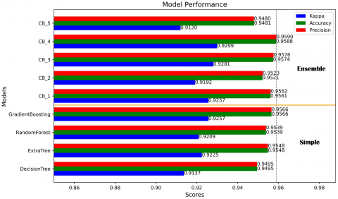
The simple models achieved accuracies of 0.9495, 0.9548, 0.9539, and 0.9566, with Kappa values of 0.9137, 0.9225, 0.9209, and 0.9257, respectively. Meanwhile, the ensemble models had accuracies of 0.9562, 0.9523, 0.9576, 0.9590, and 0.9480, with Kappas of 0.9257, 0.9192, 0.9281, 0.9299, and 0.9120. The Gradient-Boosting algorithm of the simple models stood out as the best, with a Kappa, Accuracy, Precision, Recall, and F-measure of 0.9257, 0.9566, 0.9566, 0.9566, and 0.9565. The best combination of the assembled models was the Ensemble CB_4 model, which consisted of the Decision-Tree and Gradient-Boosting algorithms. It achieved a Kappa of 0.9299, Accuracy of 0.9588, Precision of 0.9590, Recall of 0.958, and F-measure of 0.9587. The other models achieved Kappa scores of 0.9285 and 0.9565, respectively.
The models, particularly the Gradient-Boosting model, demonstrate exceptional accuracy and predictive ability, as shown in Table 12. Ensemble models also show promise, with certain combinations, such as Decision Tree + Gradient Boosting, exhibiting notably superior performance compared to other ensembles. These findings are comparable to those of Fernández-Delgado et al. [38] compared 179 algorithms across 17 distinct families using 121 datasets. The analysis revealed that random forest techniques consistently exhibited superior performance compared to other learning methodologies, particularly when utilizing random forest and boosting with 1,000 trees, which achieved the highest average ranking among the various algorithms assessed. These findings indicate that both straightforward and ensemble models are effective in predicting seismic vulnerability in masonry housing.
Figure 6 shows a detailed performance comparison of the predictive models. The section includes the 'Simple' models, such as Decision Tree, Extra Tree, Random Forest, Gradient Boosting, and 'Ensemble' models featuring the combined models CB_1 to CB_5. Each bar represents the models' scores on three key metrics: Kappa, Accuracy, and Precision. The values are close to each other and mostly above 0.90. The CB_4 model achieved the highest accuracy at 95.90%, outperforming both the other combinations and simple models.
The study's results surpass the models proposed by other authors. Firmansyah et al. [2] achieved an F1 score of 84.33% using a CNN model, while Bektaş and Kegyes-Brassai [11] obtained 68% using neural networks. In contrast, Bessason et al. [3] used a logistic zero inflation beta regression model and achieved 90%.
Table 12. Performance indicator for seismic vulnerability prediction models
|
Type |
Model |
Kappa |
Accuracy |
Precision |
Recall |
F-measure |
|
Simple |
Decision Tree |
0.9137 |
0.9495 |
0.9495 |
0.9495 |
0.9494 |
|
Extra Tree |
0.9225 |
0.9548 |
0.9548 |
0.9548 |
0.9547 |
|
|
Random Forest |
0.9209 |
0.9539 |
0.9539 |
0.9539 |
0.9537 |
|
|
Gradient Boosting |
0.9257 |
0.9566 |
0.9566 |
0.9566 |
0.9565 |
|
|
Ensemble |
Extra Tree + Decision Tree + Gradient Boosting + Random Forest |
0.9257 |
0.9561 |
0.9562 |
0.9561 |
0.9561 |
|
Extra Tree + Decision Tree + Random Forest |
0.9192 |
0.9521 |
0.9523 |
0.9521 |
0.9522 |
|
|
Extra Tree + Random Forest + Gradient Boosting |
0.9281 |
0.9574 |
0.9576 |
0.9574 |
0.9575 |
|
|
Decision Tree + Gradient Boosting |
0.9299 |
0.9588 |
0.9590 |
0.9588 |
0.9587 |
|
|
Decision Tree + Random Forest |
0.9120 |
0.9481 |
0.9480 |
0.9481 |
0.9480 |
Figure 6. Comparison of the performance of single and assembled models
Figure 7 presents the confusion matrix of the performance of the four simple classification models (Gradient Boosting, Random Forest, Extra Tree, and Decision Tree) in the prediction of the seismic vulnerability classes. The levels of classification were designated as High, Moderate, and Low. In the High class, the Decision Tree model demonstrated the greatest accuracy with 127 correct predictions, followed by Gradient Boosting with 126, Extra Tree with 125, and Random Forest with 121. In the Moderate class, the Extra Tree model achieved 567 correct predictions, closely followed by the Random Forest model with 566, the Gradient Boosting model with 565, and the Decision Tree model with 558. In the Low class, the performance of the models is comparable, with Gradient Boosting and Random Forest achieving 389 correct predictions, while Extra Tree and Decision Tree achieve 386 and 387, respectively. These results demonstrate a high level of accuracy across all models, with the Decision Tree model exhibiting the highest level of accuracy in the High class, while the Extra Tree and Random Forest models demonstrated the greatest accuracy in the Moderate class.
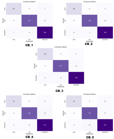
Figure 8 illustrates the performance of the five assembled models (CB_1 to CB_5) in the prediction of seismic vulnerability, categorized as High, Moderate, and Low. In the High class, models CB_2 and CB_3 exhibited the highest number of correct predictions, with 88 each, while CB_5 demonstrated the lowest performance, with 82 correct predictions. In the Moderate class, model CB_4 stands out with 370 correct predictions, followed by CB_1 and CB_2 with 366, CB_3 with 364, and CB_5 with 362. In the Low class, all models exhibited comparable performance, with CB_5 achieving the highest accuracy with 270 correct predictions. The results demonstrate a high level of accuracy for model CB_4 in the Moderate class and for CB_2 and CB_3 in the High class.
A comparison of the simple and ensemble models reveals that the CB_4 ensemble model accurately predicts the seismic vulnerability classes. The simple models tend to exhibit greater consistency overall, while the assembled models demonstrate greater specialization in the different classes. These findings underscore the importance of selecting an appropriate classification model according to the specific needs of seismic vulnerability analysis. The correct identification of high, moderate, and low areas is essential for the implementation of effective mitigation strategies and the optimization of resources in seismic risk management.
Figure 7. Confusion matrix of simple models
Figure 8. Matrix of confusion of the assembled models
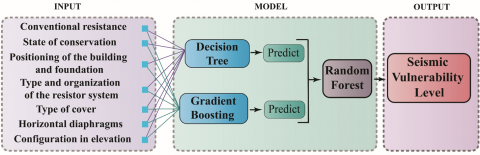
Figure 9 shows the structure of the assembled model. Seven input variables were selected: Conventional resistance, State of conservation, Positioning of the building and foundation, Type and organization of the resistor system, Type of cover, Horizontal diaphragms, and Configuration in elevation. These variables provide additional information for the output variable. The CB_4 model assembly comprises a Decision Tree and Gradient-Boosting machine learning algorithms that individually predict seismic vulnerability, resulting in two outputs. These outputs are then processed by the Random Forest meta-classifier, which consolidates them to provide an overall result that reflects the level of seismic vulnerability.
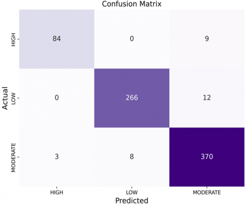
Figure 10 displays the confusion matrix of the best model (CB_4), which was obtained during validation with 20% of the database. The matrix shows that 35.24% of the dwellings were correctly classified as Low level, while 11.30% were correctly classified as High level. However, only 49.20% of the dwellings were correctly classified as moderate level. According to the confusion matrix, 1.06% of the dwellings in the High level were misclassified as Moderate level.
This model offers a more precise and reliable evaluation of seismic vulnerability. It can process large amounts of data for large-scale assessments without incurring high computational costs. Its accuracy rate of 95.90% surpasses that of other models in the literature. As a result, it was utilized to estimate the seismic vulnerability of the Pueblo Libre sector in Jaen, Cajamarca, Peru.
Figure 9. Structure of the CB_4 Model Assembly
Figure 10. Confusion matrix of the CB_4 model
4.4 Application of the validated model to the study area
After the validation of the CB_4 model, the seismic vulnerability of the sector Pueblo Libre, Jaen, Cajamarca, Peru, was estimated, evaluating 67 closed masonry houses, the parameters of the variables: Conventional resistance, state of conservation, positioning of the building and foundation, type and organization of the resistance system, type of cover, horizontal diaphragms and configuration in elevation were collected and entered into the model, obtaining a level of vulnerability in qualitative scale, of high (1. 48%), moderate (32.85%) and low (65.67%) as Ortega et al. [10], who used the same scale with other variables. Figure 11 shows in the rows the level of vulnerability and in the columns, the masonry houses evaluated at different points of the Pueblo Libre sector.
The predominant vulnerability level observed in the Pueblo Libre sector was classified as low to moderate. These findings align with the city's historical context, the anthropogenic attributes of its populace, and the degree of exposure to seismic events. This notion is corroborated by Izquierdo-Horna et al [1], who obtained a vulnerability level of very high and high in the city of Pisco. In addition, the variable's type and organization of the resistance system, conventional resistance, positioning of the building and foundation rated as B and C, and the horizontal diaphragms, configuration in elevation, type of cove, and state of conservation rated as A and B are those that determine the geometric, constructive, structural and environmental characteristics of the closed masonry houses of the sector in the event of a seismic event. It has been determined that a house has a high level of vulnerability and is prone to collapse during a seismic event. Given these risks, mitigation measures were proposed, such as structural reinforcement, continuity of structural elements, demolition of houses with cracks, and structural and construction advice for homeowners. The seismic vulnerability map, shown in Figure 12, was created using the Geographic Information System (GIS) following the methodology of Formisano et al [24] and Sauti et al [5]. The map indicates that the majority of houses have a low to moderate level of vulnerability, with over 32% falling into this category. On the right, two additional maps are presented: one for the Department of Cajamarca and another for Peru, both showing the location of the study area. The map legend indicates the High vulnerability level in red, Moderate in yellow, and Low in green.
Figure 11. Seismic vulnerability level of Pueblo Libre sector, Jaen, Cajamarca, Peru
Figure 12. Seismic vulnerability map of Pueblo Libre sector, Jaen, Cajamarca, Peru
This research proposes an innovative methodology for determining the seismic vulnerability of confined masonry dwellings. The methodology employs ensemble algorithms to automate the assessment, distinguishing itself from other methodologies in its ability to identify hidden patterns in the data.
The data-driven approach developed integrates parameters of the structural and geometric characteristics of masonry dwellings, which differs significantly from conventional methods based on linear equations. Two distinct model types were developed: simple and ensemble. Among the simple models, the Gradient-Boosting algorithm exhibited the highest degree of accuracy, with a score of 0.9566. Among the ensemble models, CB_4 (decision tree + gradient boosting) exhibited the highest degree of accuracy, achieving a score of 0.9590. This model was identified as the most accurate model for estimating seismic vulnerability, exhibiting a significant enhancement in the precision of the assessments.
The level of vulnerability obtained on a qualitative scale is classified as high (1.48%), moderate (32.85%), and low (65.67%) when applying the CB_4 ensemble model to the Pueblo Libre sector of Jaen (Peru). The ability to automate the evaluation of the dataset allows for the implementation of preventive measures and response planning for potential large seismic events. These models serve as essential tools for providing accurate and detailed assessments of seismic vulnerability, thereby facilitating decision-making processes.
For future research, it is recommended that these methods be applied to other types of structures and in different geographical contexts to validate and extend the generalization of the results. Furthermore, it would be advantageous to examine the integration of real-time data and the utilization of deep learning techniques to enhance the precision and responsiveness of the models. The implementation of hybrid approaches combining different ensemble algorithms could provide new insights and enhance the robustness of seismic evaluations.
[1] Izquierdo-Horna, L., Zevallos, J., Yepez, Y. (2022). An integrated approach to seismic risk assessment using random forest and hierarchical analysis: Pisco, Peru. Heliyon, 8(10): 1-9. https://doi.org/10.1016/j.heliyon.2022.e10926
[2] Firmansyah, H.R., Sarli, P.W., Twinanda, A.P., Santoso, D., Imran, I. (2024). Building typology classification using convolutional neural networks utilizing multiple ground-level image processes for city-scale rapid seismic vulnerability assessment. Engineering Applications of Artificial Intelligence, 131: 107824. https://doi.org/10.1016/j.engappai.2023.107824
[3] Bessason, B., Bjarnason, J.Ö., Rupakhety, R. (2020). Statistical modeling of seismic vulnerability of RC, timber, and masonry buildings from complete empirical loss data. Engineering Structures, 209: 109969. https://doi.org/10.1016/j.engstruct.2019.109969
[4] Sauti, N.S., Daud, M.E., Kaamin, M., Sahat, S. (2023). A comprehensive review of holistic indicators for seismic vulnerability assessment of Malaysia. International Journal of Disaster and Natural Hazards Engineering, 18(3): 631-642. https://doi.org/10.18280/ijdne.180315
[5] Sauti, N.S., Daud, M.E., Kaamin, M. (2020). Construction of an integrated social vulnerability index to identify spatial variability of exposure to seismic hazard in Pahang, Malaysia. International Journal of Disaster and Natural Hazards Engineering, 15(3): 365-372. https://doi.org/10.18280/ijdne.150310
[6] Neves, F., Costa, A., Vicente, R., Oliveira, C.S., Varum, H. (2012). Seismic vulnerability assessment and characterization of the buildings on Faial Island, Azores. Bulletin of Earthquake Engineering, 10(1): 27-44. https://doi.org/10.1007/s10518-011-9276-0
[7] Pasqual, F., Berto, L., Faccio, P., Saetta, A., Talledo, D. A. (2023). Seismic vulnerability assessment of RC buildings at compartment scale: The use of CARTIS form. Procedia Structural Integrity, 44: 203-210. https://doi.org/10.1016/j.prostr.2023.01.027
[8] Briceño, C., Moreira, S., Noel, M. F., Gonzales, M., Vila-Chã, E., Aguilar, R. (2019). Seismic vulnerability assessment of a 17th-century adobe church in the Peruvian Andes. International Journal of Architectural Heritage, 13(1): 140-152. https://doi.org/10.1080/15583058.2018.1497224
[9] Cuadra, C., Saito, T., Zavala, C. (2013). Diagnosis for seismic vulnerability evaluation of historical buildings in Lima, Peru. Journal of Disaster Research, 8(2): 320-327. https://doi.org/10.20965/jdr.2013.p0320
[10] Ortega, J., Vasconcelos, G., Rodrigues, H., Correia, M. (2019). A vulnerability index formulation for the seismic vulnerability assessment of vernacular architecture. Engineering Structures, 197: 109381. https://doi.org/10.1016/j.engstruct.2019.109381
[11] Bektaş, N., Kegyes-Brassai, O. (2024). Enhancing seismic assessment and risk management of buildings: A neural network-based rapid visual screening method development. Engineering Structures, 304: 117606. https://doi.org/10.1016/j.engstruct.2024.117606
[12] Sagi, O., Rokach, L. (2018). Ensemble learning: A survey. WIREs Data Mining and Knowledge Discovery, 8(4): e1249. https://doi.org/10.1002/widm.1249
[13] Rojas, P.P., Moya, C., Caballero, M., Márquez, W., Briones-Bitar, J., Morante-Carballo, F. (2023). Assessing and mitigating seismic risk for a hospital structure in Zaruma, Ecuador: A structural and regulatory evaluation. International Journal of Structural and Structural Engineering, 13(4): 597-610. https://doi.org/10.18280/ijsse.130402
[14] Sauti, N. S., Daud, M. E., Kaamin, M., Sahat, S. (2021). Development of an exposure vulnerability index map using GIS modeling for preliminary seismic risk assessment in Sabah, Malaysia. International Journal of Disaster and Natural Hazards Engineering, 16(1): 111-119. https://doi.org/10.18280/ijdne.160115
[15] López-Almansa, F., Montaña, M. A. (2014). Numerical seismic vulnerability analysis of mid-height steel buildings in Bogotá, Colombia. Journal of Constructional Steel Research, 92: 1-14. https://doi.org/10.1016/j.jcsr.2013.09.002
[16] Najar, I.A., Ahmadi, R., Khalik, Y.K.A., Mohamad, N.Z., Jamian, M.A.H., Najar, N.A. (2022). A framework of systematic land use vulnerability modeling based on seismic microzonation: A case study of miri district of Sarawak, Malaysia. International Journal of Disaster and Natural Hazards Engineering, 17(5): 669-677. https://doi.org/10.18280/ijdne.170504
[17] Talledo, D.A., Federico, R., Rocca, I., Pozza, L., Savoia, M., Saetta, A. (2023). Seismic risk assessment of a new RC-framed skin technology for integrated retrofitting interventions on existing buildings. Procedia Structural Integrity, 44: 918-925. https://doi.org/10.1016/j.prostr.2023.01.119
[18] Lin, K., Lu, X., Li, Y., Guan, H. (2019). Experimental study of a novel multi-hazard resistant prefabricated concrete frame structure. Soil Dynamics and Earthquake Engineering, 119: 390-407. https://doi.org/10.1016/j.soildyn.2018.04.011
[19] Huang, W., Zhou, X., Zhou, Q., Zhou, Z., Xu, G., Liu, S. (2024). Experimental study and numerical analysis on the failure mode of the staggered truss framing system. Engineering Structures, 307: 117878. https://doi.org/10.1016/j.engstruct.2024.117878
[20] Sadeghi, A., Moghadam, A.S., Fathi, F. (2023). Evaluation and comparison of seismic performance of industrially and traditionally constructed buildings in Iran, a case study of Yasooj. Structures, 55: 747-762. https://doi.org/10.1016/j.istruc.2023.06.032
[21] Lourenço, P.B., Roque, J.A. (2006). Simplified indexes for the seismic vulnerability of ancient masonry buildings. Construction and Building Materials, 20(4): 200-208. https://doi.org/10.1016/j.conbuildmat.2005.08.027
[22] Domaneschi, M., Zamani Noori, A., Pietropinto, M.V., Cimellaro, G.P. (2021). Seismic vulnerability assessment of existing school buildings. Computers & Structures, 248: 106522. https://doi.org/10.1016/j.compstruc.2021.106522
[23] Kassem, M.M., Mohamed Nazri, F., Noroozinejad Farsangi, E. (2020). The efficiency of an improved seismic vulnerability index under strong ground motions. Structures, 23: 366-382. https://doi.org/10.1016/j.istruc.2019.10.016
[24] Formisano, A., Landolfo, R., Mazzolani, F.M., Florio, G. (2010). A quick methodology for seismic vulnerability assessment of historical masonry aggregates. In COST C26 Final Conference "Urban Habitat Constructions under Catastrophic Events", Naples. https://doi.org/10.13140/2.1.1706.3686
[25] Chieffo, N., Formisano, A., Mochi, G., Mosoarca, M. (2021). Seismic vulnerability assessment and simplified empirical formulation for predicting the vibration periods of structural units in aggregate configuration. Geosciences, 11(7): 7. https://doi.org/10.3390/geosciences11070287
[26] Chieffo, N., Formisano, A., Landolfo, R., Milani, G. (2022). A vulnerability index-based approach for the historical center of the city of Latronico (Potenza, Southern Italy). Engineering Failure Analysis, 136: 106207. https://doi.org/10.1016/j.engfailanal.2022.106207
[27] Mantovani, R. G., Horváth, T., Cerri, R., Vanschoren, J., de Carvalho, A.C.P.L.F. (2016). Hyper-parameter tuning of a decision tree induction algorithm. In 2016 5th Brazilian Conference on Intelligent Systems (BRACIS), Recife, Brazil, pp. 37-42. https://doi.org/10.1109/BRACIS.2016.018
[28] Gavel, A., Andrae, R., Fouesneau, M., Korn, A.J., Sordo, R. (2021). Estimating [α/Fe] from Gaia low-resolution BP/RP spectra using the ExtraTrees algorithm. Astronomy & Astrophysics, 656: A93. https://doi.org/10.1051/0004-6361/202141589
[29] Palomino Ojeda, J.M., Quiñones Huatangari, L., Cayatopa Calderón, B.A. (2023). Employing data mining techniques for engineering soil classification: a unified soil classification system approach. Mathematics in Engineering and Physical Sciences, 10(6): 1994-2002. https://doi.org/10.18280/mmep.100609
[30] Chen, Y., Jia, Z., Mercola, D., Xie, X. (2013). A gradient boosting algorithm for survival analysis via direct optimization of concordance index. Computational and Mathematical Methods in Medicine, 2013: e873595. https://doi.org/10.1155/2013/873595
[31] Friedman, J.H. (2002). Stochastic gradient boosting. Computational Statistics & Data Analysis, 38(4): 367-378. https://doi.org/10.1016/S0167-9473(01)00065-2
[32] Angjeliu, G., Cardani, G., Garavaglia, E. (2023). Rapid assessment of the seismic vulnerability of historic masonry structures through fragility curves approach and national database data. Developments in the Built Environment, 14: 100140. https://doi.org/10.1016/j.dibe.2023.100140
[33] Xu, W., Kang, Y.F., Chen, L.C., Wang, L.Q., Qin, C.B., Zhang, L.T., Liang, D., Wu, C.Z., Zhang, W.G. (2023). Dynamic assessment of slope stability based on multi-source monitoring data and ensemble learning approaches: A case study of Jiuxianping landslide. Geological Journal, 58(6): 2353-2371. https://doi.org/10.1002/gj.4605
[34] Li, C., Wang, L., Li, J., Chen, Y. (2024). Application of multi-algorithm ensemble methods in high-dimensional and small-sample data of geotechnical engineering: A case study of swelling pressure of expansive soils. Journal of Rock Mechanics and Geotechnical Engineering. https://doi.org/10.1016/j.jrmge.2023.10.015
[35] Su, J., Wang, Y., Niu, X., Sha, S., Yu, J. (2022). Prediction of ground surface settlement by shield tunneling using XGBoost and Bayesian Optimization. Engineering Applications of Artificial Intelligence, 114: 105020. https://doi.org/10.1016/j.engappai.2022.105020
[36] Palomino Ojeda, J. M., Pérez Herrera, N., Quiñones Huatangari, L., Cayatopa Calderón, B.A. (2023). Determination of steel area in reinforced concrete beams using data mining techniques. Revue d'Intelligence Artificielle, 37(4): 817-824. https://doi.org/10.18280/ria.370401
[37] Dietterichl, T.G. (2002). Ensemble Learning. In M. Arbib (Ed.), The Handbook of Brain Theory and Neural Networks, MIT Press, 405-408. https://philpapers.org/rec/ARBTHO.
[38] Fernández-Delgado, M., Cernadas, E., Barro, S., Amorim, D. (2014). Do we need hundreds of classifiers to solve real-world classification problems? Journal of Machine Learning Research, 15(1): 3133-3181. https://jmlr.org/papers/v15/delgado14a.html.