Hayder Osamah Dawood Alkhalidi*![]() | Semih Bilgen
| Semih Bilgen![]()
© 2024 The authors. This article is published by IIETA and is licensed under the CC BY 4.0 license (http://creativecommons.org/licenses/by/4.0/).
OPEN ACCESS
A novel deep learning architecture, BSRDNN (brain signal recognition deep neural network), based on a one-dimensional convolutional neural network model (1D-CNN) and artificial neural network (ANN), is proposed for drowsiness detection from single-channel electroencephalographic (EEG) data. The effectiveness of the method is shown using the MIT/BIH polysomnographic EEG dataset (MIT/BIH-PED) with more than 80h long-term EEG data collected by a single electrode. EEG signals for 16 subjects were classified by BSRDNN as wakefulness, drowsiness, and sleep. BSRDNN was used via two approaches: Option 1 consists of feature extraction and classification by deep learning; in Option 2, feature and classification are performed by machine learning algorithms, naïve Bayes (NB), k-nearest neighbours (KNN), random forest (RF), and stochastic gradient descent (SGD). Combined-subject validation was applied extraction to enhance the performance of the proposed technique. Simulations demonstrated better performance in terms of accuracy, recall, F1-score and precision compared to the current state-of-the-art techniques applied to the same dataset: We obtained 92.31% overall accuracy in Option 1, and 94.8-100% in Option 2. The proposed novel BSRDNN model demonstrates clear superiority over those featured in published research that used the same MIT/BIH-PED dataset. It can perform its designated task with less trainable parameters and arithmetic operations compared to other models, resulting in faster training and testing phases. This enhanced speed facilitates quicker drowsiness detection, thereby reducing the overall time required for the process.
single channel drowsiness detection, novel deep learning architecture, machine learning, one dimensional convolutional neural network (1D-CNN)
Drowsiness impairs the brain's responsiveness, which is crucial for speedy decision-making. Drowsiness is one of the primary contributors to the incidence of traffic accidents following high-speed driving or alcohol intake [1]. A common and brief condition of inattention that occurs when a person transitions from being awake to being asleep is referred to as drowsiness. Drowsiness detection has been an increasingly popular topic in recent years, especially since vehicle makers study and develop early warning systems for driver drowsiness. Subjective, vehicle, behaviour, and physiology-based sleepiness detection methods have been presented [2-6]. Physiology-based sleepiness detection technologies are becoming progressively more accurate and efficient due to biological detection and sensor improvement [6, 7]. Physiology-based sleepiness detection uses electrophysiological signals such as electrooculographic (EOG), electrocardiographic (ECG), and electroencephalogram (EEG) data or combinations of these signals [8-10]. EEG may capture millisecond events and measure a person's mental tension, drowsiness, and emotional state [11, 12]. The EEG is not prohibitively expensive and may quickly and painlessly be obtained from the scalp, making it popular in drowsiness and sleep investigations [13, 14]. Earlier drowsiness detection techniques collected EEG signals from several brain regions using multi-channel EEG equipment [15]. These techniques may improve the accuracy of sleep detection. However, the following issues can arise from the capacity to obtain vast volumes of electrical brain data rapidly via EEG signals:
•The use of multi-dimensional data requires a large amount of storage space.
•Excessive computation time.
•Sensors for collecting multi-channel data are expensive to produce.
•Multiple sensors on a driver’s skull are annoying and impractical.
In recent years, there has been a competition among researchers to improve the accuracy of drowsiness detection. This improvement is often achieved by devising new and novel methods for extracting features or by combining multiple features from different physiological signals across various domains. Researchers have explored handcrafted-engineered feature extraction methods [16-25] and fully automated approaches [26-33] using deep learning techniques. Upon reviewing existing literature and comparing works on the MIT/BIH-PED dataset for drowsiness detection, several studies stand out. For instance, the study [20] and the studies [22-24] focused on the frequency domain, employing methods such as fast Fourier transform (FFT), power spectral density (PSD) and wavelet transform (WT) for signal processing and feature extraction, obtaining good accuracies ranging from 83%-86.5% and 90.27%, 88.80% and 87.20%, respectively. In the studies [18, 19], both time and frequency domains were explored using WT and PSD, achieving accuracies between 83.6%-87.4% and 81.7%-86.5%. A remarkable accuracy score of 92.28% for sleepiness detection was reported [21]. Adaptive Hermite decomposition (AHD) was used in the time-frequency domain; the researchers worked on entropies in the process of signal processing and feature extraction and obtained an accuracy of 85.51% [25]. The MIT/BIH-PED signal was converted to pictures, and transfer learning (ResNet, AlexNet and VGG UNet) was utilised to identify a subject’s tiredness, with 97.92% and 94.31% accuracy, respectively [26, 27]. Adaptive variational mode decomposition (AVMD) was applied to analyse EEG signals and decompose them into several modes [16]; the features were extracted using a different entropy method. An ensemble-boosted tree classifier was utilised to obtain a higher accuracy of 97.19%. A unique hybrid technique was created to extract combination features from biomedical signals using blood and MIT/BIH-PED signals; the researchers achieved 99.01% accuracy [17]. A combination of MIT/BIH-PED and EOG hybrid novel feature extraction was used; the researchers utilised a gradient boosting decision tree (GBDT) as a classifier to achieve 91.34% accuracy [34]. The most extractable features of MIT/BIH-PED and ECG signals were combined to achieve 99.93% accuracy [35]. A deep learning architecture based on an attention mechanism combining convolutional layers, LSTM, and 1D-residual blocks was proposed; using Bi-GRU for classification and MIT/BIH-PED, the researchers achieved 98.38% accuracy for two classes: Awake and drowsiness [36]. To address limitations found in previous studies, we present a new deep learning architecture called BSRDNN that is built on a 1D-CNN and an ANN for drowsiness detection using single-channel EEG data from MIT/BIH-PED. The BSRDNN processes single-channel EEG data instead of using hybrid physiological signals to reduce complexity, computation time and mathematical operations resulting from pre-processing and feature extraction [17, 34-36]. It can extract features without converting them into 2D images [26, 27] or relying on handcrafted-engineered feature extraction methods [16-25]. Moreover, BSRDNN reduces arithmetic operation time and total trainable parameters compared to parallel models [26-30, 37]. BSRDNN was applied using two approaches: Option 1 performs feature extraction and classification using deep learning, while Option 2 consists of feature extraction and classification using machine learning algorithms (NB, KNN, RF and SGD). By identifying the appropriate and discriminant features extracted by the novel BSRDNN, our work classified the MIT/BIH-PED data into three categories: awakeness, drowsiness and sleep. The proposed novel BSRDNN model demonstrates clear superiority over those featured in published research that used the same MIT/BIH-PED dataset. It can perform its designated task with less trainable parameters and arithmetic operations compared to other models, resulting in faster training and testing phases. This enhanced speed facilitates quicker drowsiness detection, thereby reducing the overall time required for the process.
The rest of this paper is organised as follows: Section 2 explains the methodology and pre-processing applied to the dataset and the structure of the novel BSRDNN. Section 3 illustrates and provides an overview of the simulation and the metrics used to evaluate our approach, the training and testing phases, and the results that we obtained compared to state-of-the-art studies that worked on MIT/BIH-PED. Finally, Section 4 presents the discussion, conclusion, limitations and recommendations for future work, respectively.
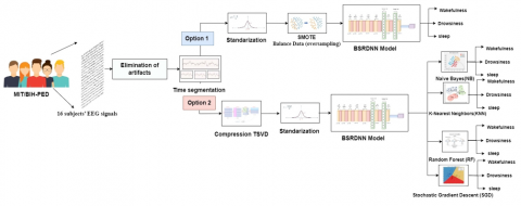
After pre-processing the MIT/BIH-PED single-channel EEG data to remove artefacts, two filters were applied: a notch filter to eliminate power line interference and a bandpass filter ranging between 0.15 and 45 Hz to remove insignificant noise. After that, time segmentation was applied to the data on 16 subjects available in MIT/BIH-PED. The data were segmented into 30 s windows depending on the label. Figure 1 shows the two Options used to implement the proposed method. In Option 1, BSRDNN was used for feature extraction and classification after scaling and applying the data oversampling algorithm to the dataset. In Option 2, feature extraction and classification were performed by machine learning algorithms, specifically NB, KNN, RF and SGD. These blocks are explained in detail below.
Figure 1. The main blocks used in Options 1 and 2
2.1 Dataset and pre-processing steps
We used the pre-recorded MIT/BIH-PED [38] data set, collected by a single electrode and this data is open to the public and may be found on the Physionet.org website, which is presented by the National Institutes of Health (NIH). Signals in that data set were recorded at a frequency of 250 Hz, and the electrodes C3-O1, C4-A1, and O2-A1 collected the sleep EEG data from 16 subjects’ left or right scalps, depending on the active area in the subjects’ brain. The EEG data were classified into three categories: awake (W), non-rapid eye movement sleep (NREM), and rapid eye movement (REM). Awake (W) is a state of consciousness in which a person is alert and able to do daily tasks.
The second type of sleep, the NREM, is divided into four stages. Stage 1 (S1) is associated with drowsiness; it represents a transition between waking and sleeping. The subsequent stages, such as Stage 2 (S2), Stage 3 (S3), and Stage 4 (S4), are linked to different states of sleep [39]. REM sleep, or stage R is a sleep stage characterized by the random rapid movement of the eyes. Artefacts interfere with EEG by reducing information from its signals. It was essential to remove the artefacts completely from the MIT/BIH-PED without distorting the information in the EEG signal relating to brain activity. Hardware artefacts were removed from every epoch (30 seconds) in the data by using a notch filter to eliminate the power line interference and a band-pass filter ranging between 0.15 Hz-45 Hz to remove nonsignificant high-frequency noise as shown in the Algorithm 1. The filters were applied in succession to all epochs to eliminate resonance noise and eye blink artefacts [20, 23, 29, 30].
|
Algorithm 1. Algorithm for elimination artifacts form EEG signals |
|
All subject's input: EEG [16] // Entered all EEG signals for 16 subjects. Subject_counter = 1 // Initialization Subject counter with value 1. While (Subject_counter <= 16) // While loop to take all 16 subjects. EEG_data = EEG (Subject_counter) // Initialization EEG data variable with all 16 subjects. MLength = length (EEG_data) // measure the EEG length signal for all 16 subjects Counter = 1 // Initialization Counter variable with value 1. Division = MLength / 7500 // Initialization the Division variable with total length of EEG signal over 7500 sample (30 sec) Column = 1 // Initialization Column variable with value 1. While (Counter <= Division) // while loop to take every 7500 sample to sec and make filtering to them. EEG = Perform filtering using 0.1 Hz to 45 Hz // filter band-pass filter applied to remove the non-significant high frequency noise. EEG.hand = Perform filtering using 0.15 Hz to 45 Hz // band-pass filter applied to remove the non-significant high frequency noise. Column = Column+7500 // take the next 7500 sample (30 Sec) Counter++ // Increase the Counter variable. END while END while |
2.2 Data segmentation
Two important sleep quality standards exist: Rechtschaffen and Kales produced the first in 1968, while the American Academy of Sleep Medicine (AASM) developed the second in 2007 [40]. The MIT/BIH-PED was assessed based on the first standard, and the data were labelled every 30 s. At 250 Hz, each 30 s of data contains 7500 samples, resulting in 10258 raw samples with 7500 (30 s) columns for 16 subjects.
2.3 Compression of raw EEG data using truncated singular value decomposition
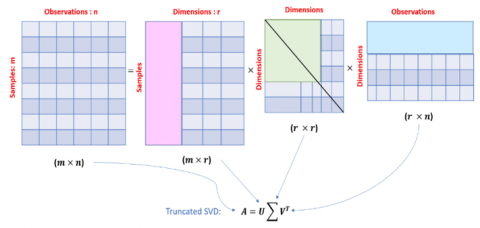
Truncated singular value decomposition (TSVD) is a method of matrix factorization that divides matrix $\mathrm{A}$ into the three matrices U, $\sum$, and V, as shown in Figure 2. TSVD corresponds to the operation $\boldsymbol{A}=\boldsymbol{U} \sum \boldsymbol{V}^T$ where $\boldsymbol{A}$ represents an $(\boldsymbol{m} \times \boldsymbol{n})$ data matrix, where $\boldsymbol{m}$ and $\boldsymbol{n}$ are the numbers of rows and columns of the samples and observations, respectively. $\boldsymbol{U}$ is the left truncated singular vector $(\boldsymbol{m} \times \boldsymbol{r})$, where $r$ represents the shortened dimension index. $\sum$ on the other hand, displays the truncated singular values of an $(\boldsymbol{r} \times \boldsymbol{r})$ matrix, and the right singular vector of an $(\boldsymbol{r} \times \boldsymbol{n})$ truncated matrix is represented as $\boldsymbol{V}^{\boldsymbol{T}}$ [41].
Figure 2. Schematic diagram of the TSVD
After segmentation into 30 s (7500 samples), we employed TSVD in Option 2. EEG signals from 7500 samples (30 s) were compressed into 25 (0.1 s), 125 (0.5 s), 250 (1 s), 375 (1.5 s), 500 (2 s), and 625 (2.5 s) samples. The TSVD technique showed us how to reduce redundant data by selecting important features based on data variance and a productive data compression method that preserves vital information in EEG data while achieving a high compression ratio.
2.4 Data scaling (Standardization)
The rescaling strategy inherent to machine learning has prevented characteristics with wider ranges from dominating others. Therefore, all EEG data inputs were rescaled to have the properties of a typical normal distribution [42]. The sample standard score was computed as Eq. (1):
$z=\left(\frac{x-\mu}{\sigma}\right)$ (1)
where, x represents the input sample or EEG data, $\mu$ signifies the mean calculated for the data or the global average, and $\sigma$ is the standard deviation. Standardization involves setting the mean to zero and the standard deviation to one to reduce computation time and improve accuracy for deep neural networks.
2.5 Imbalanced data (Oversampling data)
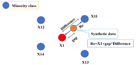
The synthetic minority oversampling technique (SMOTE) [43] is one of the most popular oversampling techniques for addressing the imbalance issue. It is a way of creating synthetic data by modifying various processes. It is one of the most prominent of these approaches; it can also balance the distribution of classes but does not provide any additional information to the model. SMOTE calculates feature vector distances for the minority class. Figure 3 shows that the difference is multiplied by a random value to balance all classes and added to the preceding feature vector.
Figure 3. Overcoming class imbalance using SMOTE
2.6 Proposed BSRDNN model
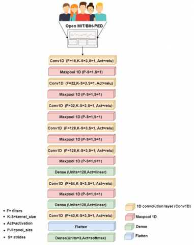
CNNs are specialized artificial neural networks for data processing and feature extraction [44-46]. To classify data, a CNN extracts features from video (3D), image (2D), or speech signal (1D) data. Each CNN model comprises a convolution layer with kernels or filters to do this. This enables the network to construct feature vectors. In our network, a pooling layer was used to minimize data dimensionality, and a dense layer was used to improve performance. CNN performs a dot product operation to develop features. The input data and filter kernel weights are used to do this. The dot product operation was entrusted to a certain kind of CNN (1D, 2D, or 3D) with a specific size of kernel based on the dimensions of the input dataset signals, which can be classified using 1D-CNN directly from raw data, reducing computational and signal transform costs. 1D-CNN requires fewer arithmetic operations than 2D-CNN. Without converting single-channel EEG inputs to 2D, it may detect tiredness. This inspired us to create our own BSRDNN, a very advanced neural network constructed using 1D-CNN and ANN (Figure 4). The baseline model for the BSRDNN’s design was based on the VGG19 net by Gallo [46]. By duplicating 1D-CNN layers with the same filter value and size, especially Conv1d (32*3) and Conv1d (128*3), this duplication of Conv1d layers resulted in increased training speed, reduced training samples per unit time and enhanced accuracy. Two layers of dense (128) neurons were placed between the convolution layers. This idea came from a DenseNet suggested by Wang et al. [47]. The concept behind this approach is to enable each layer to access the features of all preceding layers, thereby enhancing the gradient flow during training and facilitating the network’s acquisition of knowledge for improved accuracy instead of using a long short-term memory (LSTM) layer. Tables 1 and 2 describe BSRDNN layers for two Options. It is assumed that the raw EEG signals can be representative of by x and that the filter or kernel size is $K_s$. The $K_s$ samples of a specific signal window, with weights for a filter-kernel assigned at random by $K_s$, were created with new $K_s$ Qvalues by the dot product operation, as Eq. (2):
$x_{\text {new }}=\operatorname{Act}\left(x *\right.$ kernel $_{k s}+$ Bias $\left._{k s}\right)$ (2)
where,
Act: Activation function.
Bias: Bias value of kernel.
*: Convolution dot operation.
kernel: Size of filters with size $K_s$.
$x$: EEG signal within N data points $x_1, x_2 \ldots, x_N$.
In the place of the EEG, $K_s$ models, the mean of these new $K_s$ values or their largest values, were employed. This process was iterated until every sample contained in the entire signal was processed. The optimal number and size of filters affect their performance. The terms used in Figure 4 and Tables 1 and 2 are defined as follows.
Figure 4. Structure of proposed model (BSRDNN) based on hybrid 1D-CNN and ANN
Output shape: This represents the output shape in Table 1 from the first layer of Conv 1D (7498,16). The first integer, 7498 in the first row, represents the length vector after applying filter size 3 on 7500 samples (30 sec). The second integer, 16, represents the number of filters applied to the EEG signal. The other layers were calculated as in the first layer.
Parameters: These are typically the weights of the connections. In this case, these parameters were learned during the training stage and can be calculated by (((size filter*number of channel) + bias) *number of filters); in our case, (((3*1) + 1) *16) we obtained 64 in the first layer. The other layers were calculated as in the first layer.
Table 1. Summary of the proposed BSRDNN in Option 1 model based on 1D-CNN and ANN, showing computational complexity
|
Layer No. |
Layer (Type) |
Filter*Kernel Size |
UNIT SIZE |
Complexity Computational |
|
|
Parameters |
Output Shape |
||||
|
1 |
Conv 1D |
16*3 |
– |
64 |
(7498, 16) |
|
2 |
Maxpool 1D |
– |
– |
0 |
(7498, 16) |
|
3 |
Conv 1D |
32*3 |
– |
1568 |
(7496, 32) |
|
4 |
Maxpool 1D |
– |
– |
0 |
(7496, 32) |
|
5 |
Conv 1D |
32*3 |
– |
3104 |
(7494, 32) |
|
6 |
Maxpool 1D |
– |
– |
0 |
(7494, 32) |
|
7 |
Conv 1D |
128*3 |
– |
12416 |
(7492, 128) |
|
8 |
Maxpool 1D |
– |
– |
0 |
(7492, 128) |
|
9 |
Conv 1D |
128*3 |
– |
49280 |
(7490, 128) |
|
10 |
Maxpool 1D |
– |
– |
0 |
(7490, 128) |
|
11 |
Dense |
– |
128 |
16512 |
(7490, 128) |
|
12 |
Conv 1D |
64*3 |
– |
24640 |
(7488, 64) |
|
13 |
Maxpool 1D |
– |
– |
0 |
(7488, 64) |
|
14 |
Dense |
– |
128 |
8320 |
(7488, 128) |
|
15 |
Conv 1D |
40*1 |
– |
5160 |
(7488, 40) |
|
16 |
Flatten |
– |
– |
0 |
299520 |
|
17 |
Dense |
– |
3 |
898563 |
3 |
Table 2. Summary of the proposed BSRDNN model in Option 2 using TSVD 25,125,250,325,500,625, showing computational complexity
|
Layer No. & Type |
Output Shape and Parameters (Complexity Computational) for TSVD (25,125,250,325,500,625) |
||||||
|
TSVD=25 |
TSVD=125 |
TSVD=250 |
|||||
|
1 |
Conv 1D |
(23, 16) |
64 |
(123, 16) |
64 |
(248, 16) |
64 |
|
2 |
Maxpool 1D |
(23, 16) |
0 |
(123, 16) |
0 |
(248, 16) |
0 |
|
3 |
Conv 1D |
(21, 32) |
1568 |
(121, 32) |
1568 |
(246, 32) |
1568 |
|
4 |
Maxpool 1D |
(21, 32) |
0 |
(121, 32) |
0 |
(246, 32) |
0 |
|
5 |
Conv 1D |
(19, 32) |
3104 |
(119, 32) |
3104 |
(244, 32) |
3104 |
|
6 |
Maxpool 1D |
(19, 32) |
0 |
(119, 32) |
0 |
(244, 32) |
0 |
|
7 |
Conv 1D |
(17, 128) |
12416 |
(117, 128) |
12416 |
(242, 128) |
12416 |
|
8 |
Maxpool 1D |
(17, 128) |
0 |
(117, 128) |
0 |
(242, 128) |
0 |
|
9 |
Conv 1D |
(15, 128) |
49280 |
(115, 128) |
49280 |
(240, 128) |
49280 |
|
10 |
Maxpool 1D |
(15, 128) |
0 |
(115, 128) |
0 |
(240, 128) |
0 |
|
11 |
Dense |
(15, 128) |
16512 |
(115, 128) |
16512 |
(240, 128) |
16512 |
|
12 |
Conv 1D |
(13, 64) |
24640 |
(113, 64) |
24640 |
(238, 64) |
24640 |
|
13 |
Maxpool 1D |
(13, 64) |
0 |
(113, 64) |
0 |
(238, 64) |
0 |
|
14 |
Dense |
(13, 128) |
8320 |
(113, 128) |
8320 |
(238, 128) |
8320 |
|
15 |
Conv 1D |
(13, 40) |
5160 |
(113, 40) |
5160 |
(238, 40) |
5160 |
|
16 |
Flatten |
(520) |
0 |
(4520) |
0 |
(9520) |
0 |
|
17 |
Dense |
(3) |
1563 |
(3) |
13563 |
(3) |
28563 |
|
Layer No. & Type |
TSVD=325 |
TSVD=500 |
TSVD=625 |
||||
|
1 |
Conv 1D |
(373, 16) |
64 |
(498, 16) |
64 |
(623, 16) |
64 |
|
2 |
Maxpool 1D |
(373, 16) |
0 |
(498, 16) |
0 |
(623, 16) |
0 |
|
3 |
Conv 1D |
(371, 32) |
1568 |
(496, 32) |
1568 |
(621, 32) |
1568 |
|
4 |
Maxpool 1D |
(371, 32) |
0 |
(496, 32) |
0 |
(621, 32) |
0 |
|
5 |
Conv 1D |
(369, 32) |
3104 |
(494, 32) |
3104 |
(619, 32) |
3104 |
|
6 |
Maxpool 1D |
(369, 32) |
0 |
(494, 32) |
0 |
(619, 32) |
0 |
|
7 |
Conv 1D |
(367, 128) |
12416 |
(492, 128) |
12416 |
(617, 128) |
12416 |
|
8 |
Maxpool 1D |
(367, 128) |
0 |
(492, 128) |
0 |
(617, 128) |
0 |
|
9 |
Conv 1D |
(365, 128) |
49280 |
(490, 128) |
49280 |
(615, 128) |
49280 |
|
10 |
Maxpool 1D |
(365, 128) |
0 |
(490, 128) |
0 |
(615, 128) |
0 |
|
11 |
Dense |
(365, 128) |
16512 |
(490, 128) |
16512 |
(615, 128) |
16512 |
|
12 |
Conv 1D |
(363, 64) |
24640 |
(488, 64) |
24640 |
(613, 64) |
24640 |
|
13 |
Maxpool 1D |
(363, 64) |
0 |
(488, 64) |
0 |
(613, 64) |
0 |
|
14 |
Dense |
(363, 128) |
8320 |
(488, 128) |
8320 |
(613, 128) |
8320 |
|
15 |
Conv 1D |
(363, 40) |
5160 |
(488, 40) |
5160 |
(613, 40) |
5160 |
|
16 |
Flatten |
(14520) |
0 |
(19520) |
0 |
(24520) |
0 |
|
17 |
Dense |
(3) |
43563 |
(3) |
58563 |
(3) |
73563 |
1D convolution layer (Conv1D): As a modified variant of a two-dimensional convolutional neural network (2D-CNN), a 1D-CNN was recently developed in deep learning. The advantage of a 1D-CNN is that it has a minimum computation requirement owing to the design's simplicity and portability, which makes it suitable for real-time and cost-effective hardware implementation, where the convolution layer uses kernel weights of filters to transform the raw EEG data into feature maps [48].
Maxpool 1D: The layers are used to subsample each input layer by making it less complex and reducing the number of parameters that need to be learned. The cost of computing can be decreased by reducing the size of feature maps by considering their maximum values [44]. Used Stride 1 after the 1D convolution layer to preserve the original time resolution by depend on Wang et al. [49].
Flatten layer: This layer "flattens" the multidimensional data that was generated by the layers that came before it into a single vector so that it may be utilised as an input for the step that comes after it [48].
Dense layer: This is the most popular and widely used layer. The dense layer describes the connection between neurons in the next and intermediate layers [46]. In our architecture, we used three fully connected layers. To improve classification results, we used a hidden layer of 128 neurons in our model's first and second dense layers. The final neuron value for the third dense is equal to multiple classifications applied in this work, so a three-neuron is sufficient to make a classification of the EEG signals into three categories awakeness, drowsiness and sleep.
Softmax function: The Softmax function is particularly beneficial because it converts a vector of real numbers into a probability distribution of possible outcomes. A Softmax function is often used as an activation function in the output layer of NN models, which predicts a multinomial probability and may be specified as Eq. (3) [44, 48]:
$\sigma(z)_i=\frac{e^{z_i}}{\sum_{j=0}^N e^{z_i}}$ (3)
where, N is the number of classes, z is the input vector, and $\sigma(z) i$ is the output class probability.
3.1 Simulation setup
We simulated the operation of BSRDNN for drowsiness detection using MIT/BIH-PED data collected through a single channel, to classify EEG data. In Option 1, the BSRDNN model was used for feature extraction and classification of the EEG signals into wakefulness, drowsiness and sleep, and in Option 2, we used the BSRDNN model for feature extraction and machine learning algorithms (NB, KNN, RF and SGD) for classification. Application of the BSRDNN in Option 1 was carried out in the Google Colab Pro Platform that had 32 GB RAM and K80, T4 and P100 GPU for training and testing. For Option 2, the application was implemented in a Python 3.6.5 environment on a computer with an Intel Core i7- 4600M @2.90 GHz CPU with 8 GB RAM for training and testing.
3.2 Evaluation metrics for classification
The confusion matrix was used to describe the performance of a classification approach or ‘classifier’ using test data. We employed the following metrics for evaluation based on the confusion matrix: overall accuracy, sensitivity, precision and F1-score [45]. These parameters are described below.
True negative (TN): When an EEG does not have drowsy characteristics, the classifier correctly predicts that the EEG does not have drowsy characteristics.
True positive (TP): When the EEG shows signs of drowsiness, the classifier can make an accurate prediction that the EEG is in a drowsy state.
False negative (FN): The classifier makes the incorrect assumption that an EEG is not drowsy when the EEG demonstrates drowsiness.
False positive (FP): The classifier makes an inaccurate prediction that the EEG is drowsy when the EEG is not in a drowsy state.
Accuracy is a statistic that indicates the overall performance of the model across all classes. It is useful in situations in which all classes are of equal importance. It is calculated by dividing the total number of correct guesses by the total number of forecasts made.
Accuracy $=\frac{T P+T N}{T P+T N+F P+F N}$ (4)
Precision is calculated as the ratio of positive samples accurately identified to the total number of positive samples classified (either correctly or incorrectly). This measure corresponds to the model’s ability to identify whether a person identified by the model as drowsy is drowsy.
Precision $=\frac{T P}{T P+F P}$ (5)
Recall is also termed as sensitivity, an additional well-known synonym for classifier fullness. This metric assesses the effectiveness of the model in detecting sleepiness in a real-world setting.
Recall $=\frac{T P}{T P+F N}$ (6)
F1-score is the weighted average of precision and recall. This measure balances the accurate prediction rates of sleepy and alert states by combining precision and sensitivity data.
$F 1-$ score $=2 \times \frac{\text { Precision } \times \text { Recall }}{\text { Precision }+ \text { Recall }}$ (7)
3.3 Training and testing phases
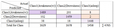
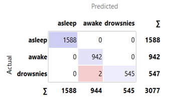
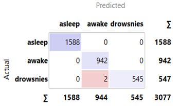
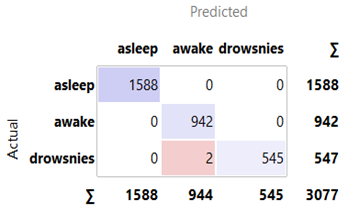
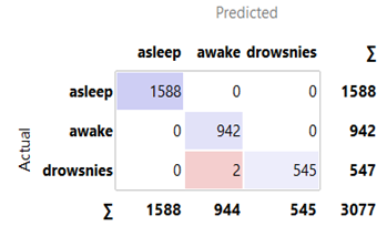
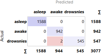
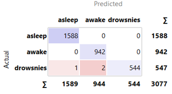
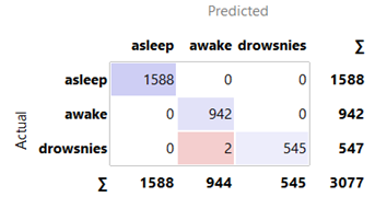
Option 1: All 10258 raw samples, 7500 (30s) columns of data, were fed into the notch and bandpass filters to eliminate power line interference and inconsequential high-frequency noise. The data was segmented into 30 s intervals depending on the label. After applying the SMOTE oversampling, the data were split into a training set comprising 70% of the data to train the BSRDNN model for feature extraction and classification of the EEG signals into wakefulness, drowsiness and sleep. The remaining 30% was reserved for testing the BSRDNN model after training. We used a hyperparameter, i.e., an Adam optimiser, with a 0.001 learning rate, 128 batch size and 50 epochs. Categorical cross-entropy was considered a loss function. In the training phase for Option 1, a total of 1.02 hours was spent on training. In the testing phase, the model needed an average time of 1 second to predict the label. Table 3 presents a summary of the results. The confusion matrix depicted in Figure 5 was obtained from Option 1.
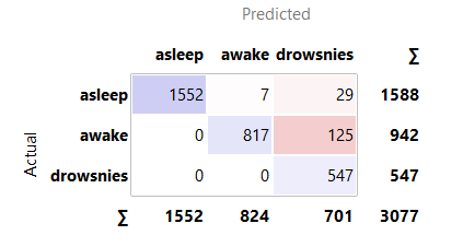
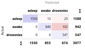
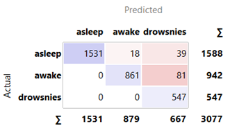
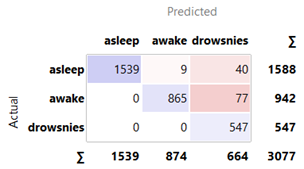
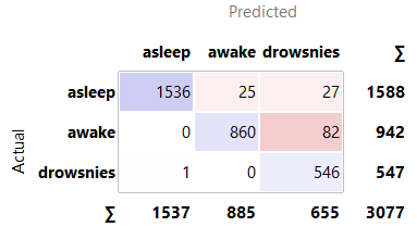
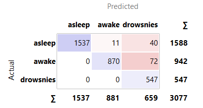
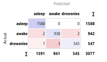
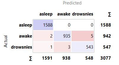
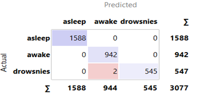
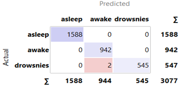
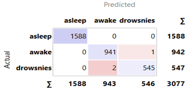
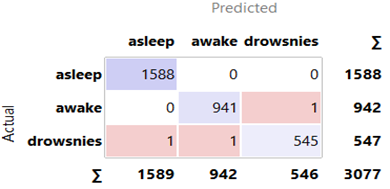
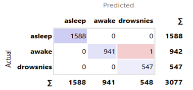
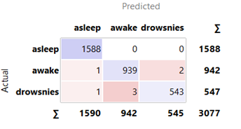
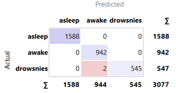
Option 2: All techniques from Option 1 were employed, with TSVD added to compress data (25, 125, 250, 375, 500, and 625 samples) by extracting key information, reducing unnecessary information, and deleting the SMOTE algorithm. Option 2 employed BSRDNN as a feature extractor and KNN, RF, SGD, and NB algorithms for classification. The BSRDNN model extracted MIT/BIH-PED features from 10258 input data with 7500 (30 s) columns. After that, the features were separated into training (70%) and test (30%) sets to assess the KNN, RF, SGD, and NB algorithms' classification abilities. The results are presented in Table 4. We used the same optimizer, learning rate of 0.001 and loss function used in Option 1 with a different batch size = 1024. In the training phase for Option 2, the total time was 0.27, 1.58, 2.1, 3.1, 4.2 and 5.2 hours for 25, 125, 250, 375, 500 and 625 samples, respectively. In the testing phase, the model needed an average time of 1 second for predicting the label. The results and confusion matrix depicted in Figures 6-9 are obtained from Option 2.
Table 3. BSRDNN (Option 1) results for feature extraction and classification
|
Status |
Precision % |
Recall % |
F1-Score % |
|
Awakeness (w) |
88% |
91% |
90% |
|
Drowsiness (Sleep stage 1) |
93% |
87% |
90% |
|
Asleep (sleep stages 2,3,4 and REM sleep) |
96% |
100% |
98% |
|
Accuracy % |
92.31% |
||
Figure 5. Confusion matrix result for option 1
Table 4. BSRDNN (Option 2) results for feature extraction and machine learning algorithms for classification
|
Naïve Bayes (NB) |
Random Forest (RF) |
||||||||
|
TSVD |
Accuracy % |
Recall % |
F1-Score |
Precision |
TSVD |
Accuracy % |
Recall % |
F1-Score |
Precision |
|
Tsvd=25 |
94.80% |
94.80% |
93.80% |
95.80% |
Tsvd=25 |
99.70% |
99.70% |
99.90% |
99.70% |
|
Tsvd=125 |
95.50% |
95.50% |
95.80% |
96.20% |
Tsvd=125 |
99.90% |
99.90% |
100.00% |
99.90% |
|
Tsvd=250 |
95.50% |
95.50% |
95.20% |
96.20% |
Tsvd=250 |
99.90% |
99.90% |
100.00% |
99.90% |
|
Tsvd=375 |
95.90% |
95.90% |
96.10% |
96.60% |
Tsvd=375 |
99.90% |
99.90% |
100.00% |
99.90% |
|
Tsvd=500 |
95.60% |
95.60% |
96.10% |
96.10% |
Tsvd=500 |
99.90% |
99.90% |
100.00% |
99.90% |
|
Tsvd=625 |
96.00% |
96.00% |
96.30% |
96.60% |
Tsvd=625 |
100.00% |
100.00% |
100.00% |
100.00% |
|
K- Nearest Neighbors (KNN) |
Stochastic Gradient Descent (SGD) |
||||||||
|
TSVD |
Accuracy % |
Recall % |
F1-Score |
Precision |
TSVD |
Accuracy % |
Recall % |
F1-Score |
Precision |
|
Tsvd=25 |
99.70% |
99.70% |
100.00% |
99.70% |
Tsvd=25 |
99.80% |
99.80% |
99.90% |
99.80% |
|
Tsvd=125 |
99.90% |
99.90% |
100.00% |
99.90% |
Tsvd=125 |
99.90% |
99.90% |
100.00% |
99.90% |
|
Tsvd=250 |
99.90% |
99.90% |
100.00% |
99.90% |
Tsvd=250 |
99.90% |
99.90% |
100.00% |
99.90% |
|
Tsvd=375 |
99.90% |
99.90% |
99.90% |
99.90% |
Tsvd=375 |
99.90% |
99.90% |
100.00% |
99.90% |
|
Tsvd=500 |
99.90% |
99.90% |
100.00% |
99.90% |
Tsvd=500 |
99.90% |
99.90% |
100.00% |
99.90% |
|
Tsvd=625 |
99.90% |
99.90% |
100.00% |
99.90% |
Tsvd=625 |
99.90% |
99.90% |
100.00% |
99.90% |
|
TSVD = 25 |
TSVD = 125 |
TSVD = 250 |
|
TSVD = 375 |
TSVD = 500 |
TSVD = 625 |
Figure 6. Confusion matrix for Naïve Bayes classifiers in Option 2
|
TSVD = 25 |
TSVD = 125 |
TSVD = 250 |
|
TSVD = 375 |
TSVD = 500 |
TSVD = 625 |
Figure 7. Confusion matrix for k-nearest neighbors Classifiers in Option 2
|
TSVD = 25 |
TSVD = 125 |
TSVD = 250 |
|
TSVD = 375 |
TSVD = 500 |
TSVD = 625 |
Figure 8. Confusion matrix for Random forest Classifiers in Option 2
|
TSVD = 25 |
TSVD = 125 |
TSVD = 250 |
|
TSVD = 375 |
TSVD = 500 |
TSVD = 625 |
Figure 9. Confusion matrix for Stochastic Gradient Descent (SGD) Classifiers in Option 2
3.4 Comparison with the state-of-the-art
To provide a fair comparison, we evaluated the performance of the proposed BSRDNN with the performance of other approaches on a benchmark consisting of MIT/BIH-PED data. Table 5 shows a detailed comparison of the metrics of our proposed BSRDNN model work with the work of the authors [16-27, 34-36]. Table 6 shows the comparison between the studies [28-30, 37] that proposed deep learning architectures based on 1D-CNN for drowsiness detection and our BSRDNN. Given that the authors used different specifications of hardware, a comparison process of the models in terms of running time will not be fair. Instead, we compare the constant total trainable parameters. The specific value for each model will give us the ability to make an appropriate comparison, as shown in Table 7. We calculate the ratio between those of other authors and our proposed model in Option 1 to show that the BSRDNN is more advantageous in terms of having less trainable parameters and arithmetic operations compared with other models.
Ratio=$\frac{\text { Total trainable patanetes for authors }}{\text { Total trainalvle parametes for propossed Option } 1}$ (8)
Table 5. Comparison of the proposed model's performance with that of other models that have been tested on the same dataset benchmark of MIT/BIH-PED
|
Methods/Publications |
Accuracy (%) |
Recall or Sensitivity (%) |
F1-score (%) |
Precision (%) |
Classes |
|
[18] |
83.6%-87.4% |
– |
– |
– |
2 |
|
[20] |
83%-86.5% |
– |
– |
– |
2 |
|
[25] |
85.51% |
85.89% |
– |
85.16% |
2 |
|
[19] |
81.7%- 86.5% |
– |
– |
– |
2 |
|
[24] |
87.20% |
– |
– |
– |
2 |
|
[23] |
88.80% |
88.55% |
– |
85.04% |
2 |
|
[22] |
90.27% |
– |
– |
– |
2 |
|
[34] |
91.34% |
– |
– |
– |
2 |
|
[21] |
92.28% |
95.45% |
93.47 |
– |
2 |
|
Proposed Option 1 |
92.31% |
91%-100% |
90%-98% |
88%-96% |
3 |
|
[26] |
94.31% |
– |
– |
– |
2 |
|
[16] |
97.19% |
97.01% |
97.60% |
98.18% |
2 |
|
[27] |
97.92% |
– |
– |
– |
2 |
|
[36] |
98.38% |
98.31% |
98.49% |
98.67% |
2 |
|
[17] |
99.01% |
99.45% |
– |
99.75 |
3 |
|
[35] |
99.93% |
99.69% |
99.93% |
99.90% |
2 |
|
Proposed Option 2 |
94.8%-100% |
94.8%-100% |
93.8%-100% |
95.8%-100% |
3 |
Table 6. Benchmarking with other studies proposed 1d-CNN for drowsiness detection
|
Authors |
Model |
Dataset |
Overall Accuracy (%) |
Recall |
F1-score (%) |
Precision (%) |
|
[28] |
1D-CNN |
sleep-EDF -2013 |
82.46%-85.39% |
40.5%-89.6% |
46.6%-90.5% |
55.0%-92.3 |
|
[30] |
1D-CNN |
Emotive EPOC+ headset device (14channels) |
90.42% |
89% |
88% |
86.51% |
|
Proposed Option 1 |
BSRDNN |
MIT/BIH-PED |
92.31% |
91%-100% |
90%-98% |
88%-96% |
|
[29] |
1D-CNN |
sleep-EDF -2013 Expanded |
94.87% |
92% |
92% |
93% |
|
[37] |
1D-CNN -LSTM |
sleep-EDF |
94.15% |
70%-97% |
65%-98% |
56%-99% |
|
Proposed Option 2 |
BSRDNN and NB, KNN, RF, SGD |
Dataset (MIT/BIH-PED |
94.8%-100% |
94.8%-100% |
93.8%-100% |
95.8%-100% |
Table 7. Comparison of the total trainable parameters for different models to Proposed Option 1
|
Authors |
Method |
Total Trainable Parameters |
Ratio |
|
Proposed Option 1 |
BSRDNN |
1,019,627 |
1 |
|
Proposed Option 2 |
BSRDNN with TSVD=25 |
122,627 |
0.12 |
|
BSRDNN with TSVD=125 |
134,627 |
0.13 |
|
|
BSRDNN with TSVD=250 |
149,627 |
0.15 |
|
|
BSRDNN with TSVD=375 |
164,627 |
0.16 |
|
|
BSRDNN with TSVD=500 |
179,627 |
0.18 |
|
|
BSRDNN with TSVD=625 |
194,627 |
0.19 |
|
|
[26] |
AlexNet |
62,378,344 |
61 |
|
VGGNet 16 |
138,423,208 |
135.8 |
|
|
[27] |
ResNet18 |
11,511,784 |
11.3 |
|
ResNet50 |
23,983,592 |
23.5 |
|
|
ResNet101 |
42,864,875 |
42 |
|
|
[28] |
1D-CNN |
29,576,658 |
29 |
|
[29] |
1D-CNN |
5,024,354 |
4.9 |
|
[30] |
1D-CNN |
14,788,329 |
14.5 |
|
[37] |
1D-CNN -LSTM |
2,450,418 |
2.4 |
In this study, we proposed a novel machine learning architecture called BSRDNN, which was able to identify drowsiness by using data from a single channel of EEG. BSRDNN can analyse and extract features automatically from raw EEG signals without the need for handcrafted-engineered features, or using transformation techniques. The performance of the proposed model was assessed with the MIT/BIH-PED data available on the Physionet.org website. Option 1 yielded an accuracy of 92.31% for combined-subject validation, and Option 2 yielded an accuracy of 94.8–100% for combined-subject validation using various algorithms for classification. Below is a summary of the merits of our work:
-As seen in Tables 5 and 6, the proposed model showed clear superiority over the published research that used the same MIT/BIH-PED dataset and other studies proposed 1d-cnn for drowsiness detection. The results were significantly improved through the proposed model, which was used in two Options: the first Option used BSRDNN as a Feature extraction and classification with a 92.31% accuracy, and the second Option combined the deep learning BSRDNN model and machine learning algorithms (NB, KNN, RF and SGD), where BSRDNN model was used for feature extraction and machine learning algorithms for classification yielded an accuracy of 94.8-100%.
-Real-time applications, such as driving, need a faster reaction time, and selecting a single-channel EEG over a multi-channel EEG accomplishes this goal.
-BSRDNN was constructed without manual feature extraction, unlike other similar studies [16, 18, 26-29]. Our method automatically extracts characteristics without human interaction. We operate directly with EEG signals without transforming them into 2D images.
-The goal in Option 2 was to improve the accuracy that we achieved in Option 1, by dedicating the BSRDNN in Option 2 to feature extraction. This, and the combination with TSVD, reduced the total number of parameters from 1,019,627 in Option 1 to around (122,627-194,627) in Option 2 as shown in Tables 1 and 2.
-TSVD achieves a high compression ratio as shown in Table 2, and preserves essential EEG information. This was evident in the results achieved with all the compressed proportions 25, 125, 250 375, 500, and 625 samples. Hence, TSVD offers considerable feature selection ability based on data variation to reduce the significant quantity of duplicate data.
-The suggested model of single-channel EEG-based drowsiness detection comparisons about other cutting-edge techniques of the same type, using the MIT/BIH-PED dataset as shown in Table 5. On the other hand, an accuracy of 99.1% has been reported based on the combination of two biomedical signals, namely blood pressure and EEG [17]. Blood pressure has some limitations, being affected by changes in facial and emotional expressions which lead to incorrect detection and extra calculations, considering its applicability, it appears that EEG is the technology that is most effective, promising, and trustworthy for detecting drowsiness [50].
-BSRDNN showed higher adaptability and a better capability to deal with single-channel data directly. Furthermore, it could extract features (up to 25, 125, 250,375, 500, 625 and 7500) automatically, which means it can be applied to other tasks via transfer learning techniques, such as in ventricular fibrillation detection and seizure detection. These techniques use single-channel data and can use BSRDNN in different applications using 1D-CNN [51].
-We achieved our primary goal of reducing the arithmetic operation time and the total number of parameters. Similar studies [28-30, 37] proposed deep learning architectures based on a 1D-CNN, but their work had drawbacks, with total parameters reaching (2.4-29.5) million and in the studies of Budak et al. [26] and Turkoglu et al. [27], they used ResNet18, ResNet50, ResNet101, AlexNet and VGGNet with (11.5-138.1) million total parameters. This means that our model requires a significantly lower number of arithmetic operations, is faster training and testing phases detect drowsiness more quickly, as the BSRDNN has 1,019,627 total parameters in Option 1 and around (122,627-194,627) in Option 2.
-Table 7 presents the ratio of total trainable parameters for different models compared to the proposed Option 1 of BSRDNN. Interestingly, the proposed Option 2 with Tsvd 25 has fewer total parameters compared to other models. This finding underscores the advantage of our proposed BSRDNN model, as it effectively reduces the total trainable parameters. This means that BSRDNN enhances the speed of both the training and testing phases, ultimately reducing the time required for drowsiness detection.
-Future results can be improved by extending the applications of BSRDNN to real driving EEG signal datasets featuring more participants. Combined with the seizure detection process, these systems can be provided in drivers’ environments via an integrated system in the vehicle.
This study on drowsiness detection has some limitations. One such limitation is the challenge of generalising the proposed model to different people and diverse environments, particularly when using EEG headsets. These headsets are often expensive, which can limit their accessibility and usage across various populations. These factors may also be sensitive to artefacts, so pre-processing should be good because these issues can affect accuracy. Furthermore, the MIT/BIH-PED dataset is primarily a laboratory non-driving EEG dataset. In the future, we hope to obtain a larger driving dataset that contains EEG signals from participants of different genders and ages.
In the future, we aim to apply BSRDNN to additional driving datasets featuring a greater number of participants and to empower the model with online learning to exploit its full potential of the model. Researchers are also encouraged to conduct additional studies on the possibility of adding predicting or forecasting to time series EEG signals and addressing related issues through other deep learning algorithms, such as the recurrent neural network (RNN), long-short-term memory (LSTM) and gated recurrent unit (GRU). Combining these algorithms with BSRDNN will facilitate the detection of drowsiness more quickly, perhaps even before it occurs. In addition, it might be possible to include a process for detecting seizures in subjects before they occur. These systems can be made available in drivers’ environments via an integrated system in a vehicle.
[1] Parekh, V., Shah, D., Shah, M. (2020). Fatigue detection using artificial intelligence framework. Augmented Human Research, 5(1): 5. https://doi.org/10.1007/s41133-019-0023-4
[2] Ahlström, C., Anund, A., Fors, C., Åkerstedt, T. (2018). Effects of the road environment on the development of driver sleepiness in young male drivers. Accident Analysis & Prevention, 112: 127-134. https://doi.org/10.1016/j.aap.2018.01.012
[3] Vinckenbosch, F.R.J., Vermeeren, A., Verster, J.C., Ramaekers, J.G., Vuurman, E.F. (2020). Validating lane drifts as a predictive measure of drug or sleepiness induced driving impairment. Psychopharmacology, 237: 877-886. https://doi.org/10.1007/s00213-019-05424-8
[4] Zhao, L., Wang, Z., Wang, X., Liu, Q. (2018). Driver drowsiness detection using facial dynamic fusion information and a DBN. IET Intelligent Transport Systems, 12(2): 127-133. https://doi.org/10.1049/iet-its.2017.0183
[5] Ramzan, M., Khan, H.U., Awan, S.M., Ismail, A., Ilyas, M., Mahmood, A. (2019). A survey on state-of-the-art drowsiness detection techniques. IEEE Access, 7: 61904-61919. https://doi.org/10.1109/ACCESS.2019.2914373
[6] Hu, X., Lodewijks, G. (2020). Detecting fatigue in car drivers and aircraft pilots by using non-invasive measures: The value of differentiation of sleepiness and mental fatigue. Journal of Safety Research, 72: 173-187. https://doi.org/10.1016/j.jsr.2019.12.015
[7] Halim, Z., Rehan, M. (2020). On identification of driving-induced stress using electroencephalogram signals: A framework based on wearable safety-critical scheme and machine learning. Information Fusion, 53: 66-79. https://doi.org/10.1016/j.inffus.2019.06.006
[8] Song, M., Li, L., Guo, J., Liu, T., Li, S., Wang, Y., Wang, J. (2020). A new method for muscular visual fatigue detection using electrooculogram. Biomedical Signal Processing and control, 58: 101865. https://doi.org/10.1016/j.bspc.2020.101865
[9] Jung, S.J., Shin, H.S., Chung, W.Y. (2014). Driver fatigue and drowsiness monitoring system with embedded electrocardiogram sensor on steering wheel. IET Intelligent Transport Systems, 8(1): 43-50. https://doi.org/10.1049/iet-its.2012.0032
[10] Wang, B., Sun, Y., Zhang, T., Sugi, T., Wang, X. (2020). Bayesian classifier with multivariate distribution based on D-vine copula model for awake/drowsiness interpretation during power nap. Biomedical Signal Processing and Control, 56: 101686. https://doi.org/10.1016/j.bspc.2019.101686
[11] Roy, Y., Banville, H., Albuquerque, I., Gramfort, A., Falk, T. H., Faubert, J. (2019). Deep learning-based electroencephalography analysis: A systematic review. Journal of Neural Engineering, 16(5): 051001. https://doi.org/10.1088/1741-2552/ab260c
[12] Al-Nafjan, A., Hosny, M., Al-Ohali, Y., Al-Wabil, A. (2017). Review and classification of emotion recognition based on EEG brain-computer interface system research: A systematic review. Applied Sciences, 7(12): 1239. https://doi.org/10.3390/app7121239
[13] Balandong, R.P., Ahmad, R.F., Saad, M.N.M., Malik, A.S. (2018). A review on EEG-based automatic sleepiness detection systems for driver. IEEE Access, 6: 22908-22919. https://doi.org/10.1109/ACCESS.2018.2811723
[14] Kamran, M.A., Mannan, M.M.N., Jeong, M.Y. (2019). Drowsiness, fatigue and poor sleep’s causes and detection: A comprehensive study. IEEE Access, 7: 167172-167186. https://doi.org/10.1109/ACCESS.2019.2951028
[15] Pouyanfar, S., Sadiq, S., Yan, Y.L., Tian, H.M., Tao, Y.D., Reyes, M.P., Shyu, M.L., Chen, S.C., Iyengar, S.S. (2018). A survey on deep learning. ACM Computing Surveys, 51(5): 1-36. https://doi.org/10.1145/3234150
[16] Khare, S.K., Bajaj, V. (2020). Entropy-based drowsiness detection using adaptive variational mode decomposition. IEEE Sensors Journal, 21(5): 6421-6428. https://doi.org/10.1109/JSEN.2020.3038440
[17] Paul, Y., Fridli, S. (2022). A hybrid approach for sleep states detection using blood pressure and EEG signal. In Lecture Notes in Electrical Engineering, pp. 119-132. 2022, https://doi.org/10.1007/978-981-16-8248-3_10
[18] Correa, A.G., Orosco, L., Laciar, E. (2014). Automatic detection of drowsiness in EEG records based on multimodal analysis. Medical Engineering & Physics, 36(2): 244-249. https://doi.org/10.1016/j.medengphy.2013.07.011
[19] Correa, A.G., Leber, E.L. (2010). An automatic detector of drowsiness based on spectral analysis and wavelet decomposition of EEG records. In 2010 Annual International Conference of the IEEE Engineering in Medicine and Biology, Buenos Aires, Argentina, pp. 1405-1408. https://doi.org/10.1109/IEMBS.2010.5626721
[20] Belakhdar, I., Kaaniche, W., Djmel, R., Ouni, B. (2016). A comparison between ANN and SVM classifier for drowsiness detection based on single EEG channel. In 2016 2nd International Conference on Advanced Technologies for Signal and Image Processing (ATSIP), Monastir, Tunisia, pp. 443-446. https://doi.org/10.1109/ATSIP.2016.7523132
[21] Taran, S., Bajaj, V. (2018). Drowsiness detection using adaptive Hermite decomposition and extreme learning machine for electroencephalogram signals. IEEE sensors Journal, 18(21): 8855-8862. https://doi.org/10.1109/JSEN.2018.2869775
[22] Boonnak, N., Kamonsantiroj, S., Pipanmaekaporn, L. (2015). Wavelet transform enhancement for drowsiness classification in EEG records using energy coefficient distribution and neural network. International Journal of Machine Learning and Computing, 5(4): 288-293. https://doi.org/10.7763/IJMLC.2015.V5.522
[23] Belakhdar, I., Kaaniche, W., Djemal, R., Ouni, B. (2018). Single-channel-based automatic drowsiness detection architecture with a reduced number of EEG features. Microprocessors and Microsystems, 58: 13-23. https://doi.org/10.1016/j.micpro.2018.02.004
[24] Anitha, C. (2019). Detection and analysis of drowsiness in human beings using multimodal signals. In Digital Business: Business Algorithms, Cloud Computing and Data Engineering, pp. 157-174. https://doi.org/10.1007/978-3-319-93940-7_7
[25] Tripathy, R.K., Acharya, U.R. (2018). Use of features from RR-time series and EEG signals for automated classification of sleep stages in deep neural network framework. Biocybernetics and Biomedical Engineering, 38(4): 890-902. https://doi.org/10.1016/j.bbe.2018.05.005
[26] Budak, U., Bajaj, V., Akbulut, Y., Atila, O., Sengur, A. (2019). An effective hybrid model for EEG-based drowsiness detection. IEEE Sensors Journal, 19(17): 7624-7631. https://doi.org/10.1109/JSEN.2019.2917850
[27] Turkoglu, M., Alcin, O.F., Aslan, M., Al-Zebari, A., Sengur, A. (2021). Deep rhythm and long short term memory-based drowsiness detection. Biomedical Signal Processing and Control, 65: 102364. https://doi.org/10.1016/j.bspc.2020.102364
[28] Khalili, E., Asl, B.M. (2021). Automatic sleep stage classification using temporal convolutional neural network and new data augmentation technique from raw single-channel EEG. Computer Methods and Programs in Biomedicine, 204: 106063. https://doi.org/10.1016/j.cmpb.2021.106063
[29] Balam, V.P., Sameer, V.U., Chinara, S. (2021). Automated classification system for drowsiness detection using convolutional neural network and electroencephalogram. IET Intelligent Transport Systems, 15(4): 514-524. https://doi.org/10.1049/itr2.12041
[30] Chaabene, S., Bouaziz, B., Boudaya, A., Hökelmann, A., Ammar, A., Chaari, L. (2021). Convolutional neural network for drowsiness detection using EEG signals. Sensors, 21(5): 1734. https://doi.org/10.3390/s21051734
[31] Bresch, E., Großekathöfer, U., Garcia-Molina, G. (2018). Recurrent deep neural networks for real-time sleep stage classification from single channel EEG. Frontiers in Computational Neuroscience, 12: 85. https://doi.org/10.3389/fncom.2018.00085
[32] Jeong, J.H., Yu, B.W., Lee, D.H., Lee, S.W. (2019). Classification of drowsiness levels based on a deep spatio-temporal convolutional bidirectional LSTM network using electroencephalography signals. Brain Sciences, 9(12): 348. https://doi.org/10.3390/brainsci9120348
[33] Lee, C., An, J. (2023). LSTM-CNN model of drowsiness detection from multiple consciousness states acquired by EEG. Expert Systems with Applications, 213: 119032. https://doi.org/10.1016/j.eswa.2022.119032
[34] Wang, W., Qin, D., Fang, Y., Zhou, C., Zheng, Y. (2024). Automatic multi-class sleep staging method based on novel hybrid features. Journal of Electrical Engineering & Technology, 19(1): 709-722. https://doi.org/10.1007/s42835-023-01570-4
[35] Rashidi, S., Asl, B.M. (2024). Strength of ensemble learning in automatic sleep stages classification using single-channel EEG and ECG signals. Medical & Biological Engineering & Computing, 62(4): 997-1015. https://doi.org/10.1007/s11517-023-02980-2
[36] Divvala, C., Mishra, M. (2024). Deep learning-based attention mechanism for automatic drowsiness detection using EEG signal. IEEE Sensors Letters, 8(3): 5501104. https://doi.org/10.1109/LSENS.2024.3363735
[37] Zhao, D., Jiang, R., Feng, M., Yang, J., Wang, Y., Hou, X., Wang, X. (2022). A deep learning algorithm based on 1D CNN-LSTM for automatic sleep staging. Technology and Health Care, 30(2): 323-336. https://doi.org/10.3233/THC-212847
[38] Goldberger, A.L., Amaral, L.A., Glass, L., et al. (2000). PhysioBank, PhysioToolkit, and PhysioNet: Components of a new research resource for complex physiologic signals. Circulation, 101(23): e215-e220. https://doi.org/10.1161/01.CIR.101.23.e215
[39] Wolpert, E.A. (1969). A manual of standardized terminology, techniques and scoring system for sleep stages of human subjects. Archives of General Psychiatry, 20(2): 246-247. https://doi.org/10.1001/archpsyc.1969.01740140118016
[40] Moser, D., Anderer, P., Gruber, G., et al. (2009). Sleep classification according to AASM and Rechtschaffen & Kales: Effects on sleep scoring parameters. Sleep, 32(2): 139-149. https://doi.org/10.5665/sleep/32.2.139
[41] Alam, M.K., Abd Aziz, A., Latif, S.A., Awang, A. (2019). Eeg data compression using truncated singular value decomposition for remote driver status monitoring. In 2019 IEEE Student Conference on Research and Development (SCOReD), Bandar Seri Iskandar, Malaysia, pp. 323-327. https://doi.org/10.1109/SCORED.2019.8896252
[42] Berriel, R.F., Lopes, A.T., Rodrigues, A., Varejao, F.M., Oliveira-Santos, T. (2017). Monthly energy consumption forecast: A deep learning approach. In 2017 International Joint Conference on Neural Networks (IJCNN), Anchorage, AK, USA, pp. 4283-4290. https://doi.org/10.1109/IJCNN.2017.7966398
[43] Chawla, N.V., Bowyer, K.W., Hall, L.O., Kegelmeyer, W.P. (2002). SMOTE: Synthetic minority over-sampling technique. Journal of Artificial Intelligence Research, 16: 321-357. https://doi.org/10.1613/jair.953
[44] Larose, D.T., Larose, C.D. (2014). Discovering Knowledge in Data: An Introduction to Data Mining (Vol. 4). John Wiley & Sons.
[45] Stancin, I., Cifrek, M., Jovic, A. (2021). A review of EEG signal features and their application in driver drowsiness detection systems. Sensors, 21(11): 3786. https://doi.org/10.3390/s21113786
[46] Gallo, C. (2015). Artificial neural networks tutorial. In Encyclopedia of Information Science and Technology, Third Edition, 6369-6378. https://doi.org/10.4018/978-1-4666-5888-2.ch626
[47] Wang, J., Chen, Y., Hao, S., Peng, X., Hu, L. (2019). Deep learning for sensor-based activity recognition: A survey. Pattern Recognition Letters, 119: 3-11. https://doi.org/10.1016/j.patrec.2018.02.010
[48] Dhillon, A., Verma, G. K. (2020). Convolutional neural network: A review of models, methodologies and applications to object detection. Progress in Artificial Intelligence, 9(2): 85-112. https://doi.org/10.1007/s13748-019-00203-0
[49] Wang, Y., Skerry-Ryan, R.J., Stanton, D., et al. (2017). Tacotron: Towards end-to-end speech synthesis. arXiv preprint arXiv: 1703.10135. https://doi.org/10.48550/arXiv.1703.10135
[50] Davidson, K.W., Prkachin, K.M., Mills, D.E., Lefcourt, H.M. (1994). Comparison of three theories relating facial expressiveness to blood pressure in male and female undergraduates. Health Psychology, 13(5): 404-11. https://doi.org/10.1037//0278-6133.13.5.404
[51] Kiranyaz, S., Avci, O., Abdeljaber, O., Ince, T., Gabbouj, M., Inman, D.J. (2021). 1D convolutional neural networks and applications: A survey. Mechanical Systems and Signal Processing, 151: 107398. https://doi.org/10.1016/j.ymssp.2020.107398