Nagababu Pachhala*![]() | Subbaiyan Jothilakshmi
| Subbaiyan Jothilakshmi![]() | Bhanu Prakash Battula
| Bhanu Prakash Battula![]()
© 2024 The authors. This article is published by IIETA and is licensed under the CC BY 4.0 license (http://creativecommons.org/licenses/by/4.0/).
OPEN ACCESS
Effective cross-platform malware categorization techniques are becoming more and more necessary as malware spreads across more systems. Conventional methods are primarily concerned with the static or dynamic aspects of malware, which often restricts their ability to identify and categorize malware on various operating systems. In this paper, we use both static and dynamic characteristics to present a unique deep learning-based method for cross-platform malware classification. Our work aims to identify the distinct features of malware on different operating systems, such as Windows, macOS, Android, and iOS. We provide a complete depiction of malware behavior by collecting both dynamic and static data, such as system calls and network traffic patterns, as well as file properties, API calls, and header information. Convolutional Neural Networks (CNN) and Gated Recurrent Units (GRU) are two components of our deep learning architecture that we use to address the inherent issues of cross-platform malware categorization. This fusion of networks enables us to effectively capture both spatial and temporal patterns present in malware samples, enhancing the accuracy of classification across platforms. To evaluate the performance of our proposed model, we employ benchmark datasets encompassing diverse malware families across different operating systems. The results demonstrate superior classification accuracy, precision, recall, and F-score compared to traditional machine learning approaches and single-feature-based models.
malware, cross-platforms, convolution neural network, gated recurrent unit, classification
With the proliferation of malware across various platforms, it has become imperative to develop effective cross-platform malware classification techniques [1]. Traditional methods typically focus on either static or dynamic features, which often restrict their ability to detect and classify malware across diverse operating systems. The research work presented in this paper introduces a novel deep learning-based approach for cross-platform malware classification [2-6] that combines both static and dynamic features to address these challenges.
The objective of this research is to capture the unique characteristics of malware targeting Windows, macOS, Android, and iOS platforms. To achieve this, the approach involves the extraction of both static and dynamic features from malware samples [7-9]. Static features encompass file attributes [10]. Application Programming Interface (API) calls, and header information, providing insights into the structural properties of the malware.
In addition to static attributes, dynamic behaviors [11-15] are analyzed by examining system calls and network traffic patterns [16]. These dynamic features shed light on how malware interacts with the underlying operating system and external networks, offering valuable information about its behavior [17-24].
To effectively tackle the complexities of cross-platform malware classification, a deep learning architecture is employed [25-32]. This architecture combines Convolutional Neural Networks (CNN) and Gated Recurrent Unit (GRU) networks [33, 34]. By utilizing this fusion of networks, the approach can capture both spatial and temporal patterns inherent in malware samples, thereby enhancing classification accuracy.
The performance of the proposed model is evaluated through experiments conducted on benchmark datasets encompassing a wide range of malware families targeting different operating systems. The results exhibit superior classification accuracy, precision, recall, and F-score when compared to traditional machine-learning approaches and single-feature-based models.
Several studies have investigated state-of-the-art methods for malware classification, with varying degrees of success. An approach for Android malware classification using static sensitive sub-graph characteristics was presented by Ou and Xu [4]. Higher-level properties of Android applications were collected by expanding function call graphs and identifying relevant vertices. By calculating a malignant score for each node, they were able to pinpoint those that were most susceptible to attack. This model performed very well against malware, with an F1-score of 97.04%.
Malware categorization was proposed by Vu et al. [7], who suggested using the encoding and organization of binary file bytes into pictures. These pictures were made from statistical and syntactic elements, and they were decorated with space-filling curves. When fed into a CNN model, these image-based features led to an impressive Hilbert curve accuracy of 93.01%.
An Android malware detection method based on machine learning was presented by Abusitta [12]. To extract API information such API calls, frequency, and sequence, they used Control Flow Graph (CFG) capabilities. The ensemble model for malware classification that included these visual cues achieved a remarkable detection accuracy of 98.98%. Using CNNs to examine AndroidManifest.xml properties, Arslan and Tasyurek [15] presented a graphical Android malware detection tool. Their model accomplished real-time inspection of mobile applications with a 96.2% malware detection rate, 97.9% precision, 98.2% recall, and 98.1% F1-score by encoding a one-or-zero vector from these variables in two dimensions for CNN training.
Kumar et al. [16] described a technique for malware classification using bitwise samples and visual cues. To extract both local and global textural properties, they converted Windows PEs into grayscale photographs. The visual characteristics were then loaded into a bespoke deep CNN model, obtaining a high-test accuracy of 98.34%. An approach for assessing non-running Android applications using an app similarity graph (ASG) was proposed by Frenklach et al. [17]. This method presupposed that functions and other generic, reusable primary components form the basis for an app's activity categorization. On standard datasets, the approach was 97.5% accurate and had an AUC of 98.7%.
PSI-Graph, a method for detecting IoT botnets by analyzing function-call graphs in executable files, was proposed by Nguyen et al. [18]. It achieved a remarkable accuracy of 98.7% on a wide variety of samples. Pektaş and Acarman [19] demonstrated possible malware operations using API call charts. By using these graphs as low-dimensional embeddings in deep networks, they were able to retain a high degree of accuracy (98.86%) while also improving network performance.
A deep transfer learning-based method for malware image classification using CNN that has been trained on ImageNet was proposed by Kumar and Janet [20]. By converting Windows PE files to grayscale images, they were able to achieve test accuracies of 93.19 percent on Microsoft datasets and 98 percent on Malimg datasets [21-31]. The MCFT-CNN model, developed by Wang and Gao [32], is a cutting-edge application of deep transfer learning to the problem of malware classification [33, 34]. This ResNet50-based model performed very well, with an accuracy of 99.18% on MalImg malware datasets, and consistently, with an accuracy of 98.63% on a bigger dataset.
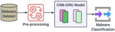
The methodology for cross-platform classification utilizing the CNN-GRU model involves a comprehensive approach to effectively capture static and dynamic features. This section is structured to highlight the key steps shown in Figure 1, starting with data pre-processing, followed by static feature representation using CNN, dynamic feature representation using GRU, and finally, an exploration of the synergistic working of the combined CNN-GRU model.
3.1 Data pre-processing
Before model development, a rigorous data pre-processing stage is undertaken. This involves cleaning, normalization, and augmentation procedures to ensure the uniformity and quality of the dataset. The objective is to enhance the robustness of the model against variations in cross-platform data, preparing it for subsequent feature extraction.
Figure 1. Cross-platform malware classification using CNN-GRU
3.2 Feature representation
The first step in the cross-platform malware detection process is feature representation. Malware samples are diverse and can exhibit unique characteristics across different platforms (e.g., Windows, macOS, Android, iOS). Therefore, the model needs to capture both static and dynamic features from these samples.
Static features include file attributes, header information, and other characteristics that do not change during program execution. On the other hand, dynamic features include system calls, network traffic patterns, and other behaviors that vary during runtime. By leveraging both static and dynamic features, the model can gain a comprehensive understanding of malware behavior on different platforms.
3.3 CNN for static features
The CNN architecture is well-suited for capturing spatial patterns in data, making it an ideal choice for processing static features. In the CNN operations, the static features ($X_{ {static }}$) are extracted by convolutional layers, to generate a feature map. An activation function, typically ReLU (Rectified Linear Unit), introduces non-linearity to the model, enabling it to learn complex relationships between features. Subsequent pooling layers down-sample the feature map, reducing its dimensions while retaining critical information. The fully connected layer further processes the pooled output to learn high-level representations.
3.4 GRU for dynamic features
The dynamic features ($X_{ {dynamic }}$) require a model capturing temporal dependencies, as the order and timing of system calls, and network activities are crucial in malware behaviour. The GRU is a type of Recurrent Neural Network (RNN) that introduces gating mechanisms to regulate information flow over time. These gates, including the reset gate (rt) and update gate (zt2), control the flow of information from the previous time step (ht-1) and the current input ($X_{ {dynamic }}$).
During the GRU operations, the reset gate determines which parts of the previous hidden state to forget, while the update gate decides how much of the new information to incorporate into the candidate hidden state ($\widehat{h_t}$). The candidate's hidden state is calculated as a combination of the reset gate and the current input. Finally, the current hidden state (ht) is updated using the candidate hidden state and the update gate.
Reset Gate (rt):
$r_t=\sigma\left(W_r \times\left[h_{t-1}, X_{\text {dynamic }}\right]+b_r\right)$ (1)
Update Gate (zt):
$z_t=\sigma\left(W_z \times\left[h_{t-1}, X_{ {dynamic }}\right]+b_z\right)$ (2)
Candidate Hidden State ($\overset{\frown}{h_t}$):
$\overset{\frown}h_t=\tanh \left(W_{\text {gru }} \times\left[r_t \times h_{t-1}, X_{\text {dynamic }}\right]+b_h\right)$ (3)
Current Hidden State (ht):
$h_t=\left(1-z_t\right) \times h_{t-1}+z_{t } * \overset{\frown}h_t$ (4)
where, $W_{c n n}$ and $b_{c n n}$ represents the weights and biases of the CNN layers, and $W_{g r u}, W_z, W_r, b_z, b_r$, and $b_h$ represents the weights and biases of the GRU layers.
3.5 Combining CNN and GRU
Once the static and dynamic features are processed separately, the model combines them for cross-platform malware detection. The outputs from the Fully Connected layer (F) and the GRU ($h_t$) are concatenated to form a comprehensive representation of malware behavior across different platforms. This combined output, referred to as Combined_Output, represents a rich feature representation that captures both spatial and temporal patterns present in the malware samples.
3.6 Classification
The Combined_Output is passed through a fully connected layer for classification. This layer maps the features to different malware classes and computes the raw scores for each class. The Sigmoid function is then applied to classify whether the operating system contains malware or not.
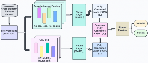
By leveraging the strengths of both CNN for static features and GRU for dynamic features, the proposed CNN-GRU model achieves effective cross-platform malware detection shown in Figure 2. The model's ability to capture unique characteristics of malware across various platforms makes it a robust and versatile solution for detecting and classifying malware threats in diverse operating environments.
Let $X_{ {static }}$ represents the static features extracted from the malware samples, and $X_{ {dynamic }}$ represents the dynamic features. Let $W_{c n n}$ and $b_{\text {cnn }}$ represent the weights and biases of the CNN layers, and $W_{g r u}, W_z, W_r, b_z, b_r$, and $b_h$ represent the weights and biases of the GRU layers.
|
Algorithm-1: Cross-Platform Malware Detection |
|
Initialization: $W_{g r u}, W_z, W_r, b_z, b_r$, and $b_h$
#CNN Operations:
|
Figure 2. CNN-GRU architecture for cross-platform malware classification
The cross-platform malware detection algorithm leverages both static and dynamic features of malware samples. The CNN extracts spatial features from the static data, while the GRU captures temporal dependencies from the dynamic data. The combined output from the CNN and GRU is used to make predictions about the malware class. Algorithm-1 can be trained on diverse datasets containing malware samples from different platforms, enabling effective cross-platform detection and classification of malware threats.
Table 1. CNN-GRU model parameters
|
Layer |
Parameter |
Description |
|
Input |
Input size |
(6248, 1087) |
|
Convolutional Layer |
Input Size |
(64, 300, 1087) |
|
Number of Filters |
64, 128, 256 |
|
|
Filter size & Stride |
3 & 1 |
|
|
Activation function |
ReLU |
|
|
Pooling layer |
Max Pooling with size 2, stride 2 |
|
|
Output shape |
(64, 36, 256) |
|
|
Flatten Layer |
Input Shape |
(64, 36, 256) |
|
Output Shape |
(589824,) |
|
|
Fully Connected Layer for CNN |
Input Shape |
(589824,) |
|
Output Shape |
(1,) |
|
|
GRU Layer |
Input Shape |
(32, 150, 128) |
|
Number of LSTM units |
128 |
|
|
Activation function |
(tanh) |
|
|
Output shape |
(32, 150, 128) |
|
|
Flatten Layer |
Input Shape |
(32, 150, 128) |
|
Output Shape |
(614400,) |
|
|
Fully Connected Layer for GRU |
Input Shape |
(614400,) |
|
Output Shape |
(1,) |
|
|
Combine Features |
(1,) |
Concatenates static and dynamic outputs |
|
Activation Function (Sigmoid) |
(1,) |
Classifies into Malware or Benign |
Table 1 outlines the architecture and parameters of a neural network model for cross-platform classification. The network comprises several layers, starting with an input layer with a size of (6248, 1087). Following this, a convolutional layer with 64, 128, and 256 filters of size 3 and a ReLU activation function is applied, along with max pooling. The output shape after this convolutional layer is (64, 36, 256). Subsequently, a flattened layer is introduced, reshaping the data to (589824,). The fully connected layer for CNN follows, transforming the input shape to (1,). A GRU layer with 128 GRU units is then applied to the input shape (32, 150, 128), producing an output shape of (32, 150, 128). Another flattens layer reshapes the data to (614400,), and a subsequent fully connected layer transforms it to (1,). The features from both the CNN and GRU pathways are combined, and a Sigmoid activation function is applied to classify the output into either malware or benign, with a final output shape of (1,).
This section delves into the experimental analysis conducted on the VxHeaven dataset for cross-platform malware analysis. The dataset serves as a comprehensive benchmark to evaluate the efficacy of the proposed CNN-GRU model in comparison to existing models, including CNN, GRU, and MCFT-CNN.
4.1 Dataset
The dataset used in this study is the "Malware static and dynamic features VxHeaven and Virus Total3 datasets." It is a multivariate dataset relevant to the field of computer science and is primarily associated with classification tasks. The dataset contains 2955 instances, where each instance represents a unique sample or file. The attributes in the dataset are of two types: integer and real values, and there are a total of 1087 attributes for each instance. The dataset is divided into three main files, each providing valuable insights into the static and dynamic properties of files on different platforms.
The first file, "staDynBenignLab.csv," consists of data extracted from 595 files on MS Windows 7 and 8, specifically obtained from the Program Files directory. It encompasses 1087 features, which capture important information related to the static and dynamic characteristics of benign files. The second file, "staDynVxHeaven2698Lab.csv," contains data from 2698 files obtained from the VxHeaven dataset. Like the previous file, it comprises 1087 features for each instance, providing valuable insights into the static and dynamic features associated with malware samples. The third file, "staDynVt2955Lab.csv," contains data extracted from 2955 files provided by Virus Total in 2018. It also includes 1087 features for each instance, representing both static and dynamic properties of malware samples.
The primary objective of this dataset is to facilitate the classification of files as either benign or malicious based on their static and dynamic features. Researchers and practitioners in the field of cybersecurity can utilize this dataset to train and evaluate machine learning models for effective cross-platform malware detection. The richness of the dataset, with its comprehensive collection of features from diverse sources, empowers the development of robust classification algorithms. This dataset plays a crucial role in advancing malware detection techniques in real-world scenarios, contributing significantly to the enhancement of cybersecurity practices, and ensuring the protection of critical systems and sensitive data.
4.2 Results and discussion
The results obtained from the experimental analysis are presented and discussed in this section. The proposed CNN-GRU model is evaluated against baseline models, including CNN, GRU, and MCFT-CNN (Malware Classification with fine-tuned convolution Neural Networks), to assess its superiority in cross-platform malware analysis. Comparative analyses encompass key performance metrics such as Accuracy, Precision, Recall, and F1-score. These metrics offer insights into the model's ability to correctly classify malware instances across diverse platforms while minimizing false positives and negatives.
The discussion delves into the strengths and limitations of each model, highlighting instances where the CNN-GRU model outperforms its counterparts. Factors such as the ability to capture both spatial and temporal features contribute to the effectiveness of the proposed model in handling cross-platform malware threats. Furthermore, the section explores specific instances where the CNN-GRU model excels, showcasing its robustness in handling dynamic and complex cross-platform malware scenarios. Insights gained from the analysis contribute to a nuanced understanding of the proposed model's capabilities and its potential advancements for future cross-platform malware detection and classification.
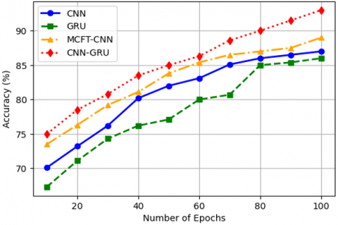
Figure 3. Accuracy
Figure 3 offers a compelling insight into the accuracy values achieved by various models, with a specific focus on the consistently superior performance of the proposed CNN-GRU model compared to other models. Accuracy is a fundamental metric in assessing classification models, measuring their ability to correctly classify data points. The data presented in Figure 3 unequivocally demonstrates that the CNN-GRU model consistently outperforms three other models—CNN, GRU, and MCFT-CNN—across all 100 epochs. At epoch 100, the CNN-GRU model attains an impressive accuracy of 93%, while the CNN, GRU, and MCFT-CNN models achieve 87%, 86%, and 89% accuracy, respectively. This remarkable performance highlights the CNN-GRU model's capacity to provide a more accurate and robust solution for cross-platform malware detection. It excels in correctly classifying malware samples, achieving a significantly higher accuracy rate compared to existing models.
The key advantage of the CNN-GRU model lies in its ability to create a comprehensive feature representation that captures both spatial and temporal patterns within malware behavior. By effectively incorporating both spatial and temporal information, the CNN-GRU model gains a more profound understanding of the intricate relationships between different features. This holistic approach enables the model to achieve higher accuracy by considering the full spectrum of characteristics that define malware samples. In contrast, the limitations of existing models, such as the CNN's focus on spatial features and the GRU's restriction to capturing sequential patterns, hinder their ability to achieve the same level of accuracy. These models may miss critical information or fail to uncover subtle relationships within the data, ultimately impacting their performance in accurately classifying malware samples.
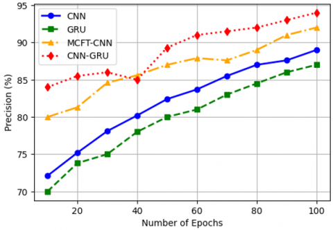
Figure 4 provides a crucial insight into the precision achieved by different models, including the proposed CNN-GRU model, during their training phases. Precision is a vital metric in the context of malware classification, as it measures the model's capability to accurately identify true positives while minimizing the occurrence of false positives. In our comparative analysis, we evaluated the precision of the CNN-GRU model alongside three other models: CNN, GRU, and MCFT-CNN. The precision of the CNN-GRU model stands out prominently with 94%. This result demonstrates the model's exceptional ability to correctly identify and classify positive malware samples among the predicted positives. A precision of 94% signifies that the CNN-GRU model excels at maintaining a high level of precision while avoiding the inclusion of false positives in its classifications.
Figure 4. Precision
Comparatively, the CNN model achieves a precision of 89%, which is commendable but falls short of the CNN-GRU's performance. The CNN model, while proficient at capturing spatial patterns in data, may encounter limitations when it comes to capturing temporal dependencies, which are crucial for accurately assessing dynamic behaviors in malware. The GRU model, on the other hand, achieves a precision of 87%, demonstrating its effectiveness in precision-oriented tasks but still slightly trailing behind the CNN-GRU model. GRU, known for its focus on sequential patterns, exhibits a strong performance but may not fully capture the intricacies of both spatial and temporal features as effectively as the CNN-GRU model. Lastly, the MCFT-CNN model achieves a precision of 92%, showcasing respectable performance but lagging behind the CNN-GRU model. The MCFT-CNN model incorporates convolutional neural networks and temporal fusion mechanisms but still doesn't match the precision offered by the CNN-GRU architecture.
The CNN-GRU model's advantage lies in its unique ability to seamlessly capture both spatial and temporal patterns. This comprehensive approach to feature extraction results in a more precise representation of malware behavior. In contrast, the limitations of existing models, such as the CNN's inability to fully grasp temporal dependencies and the GRU's primary focus on sequential patterns, may lead to less optimal precision-recall trade-offs and imbalanced classification performance.
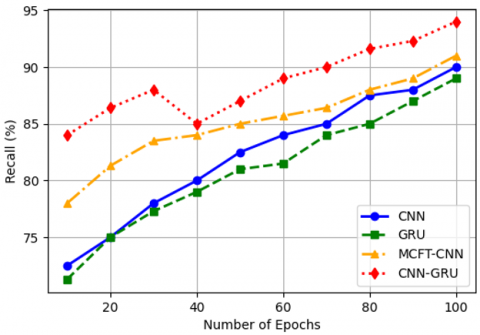
Figure 5 provides a crucial perspective on the recall performance of various models, including the proposed CNN-GRU model, throughout their training phases. Recall, often referred to as sensitivity or true positive rate, is a vital metric in malware classification as it measures the model's capability to correctly identify actual malware instances while minimizing the occurrence of false negatives. A recall score of 94% for the CNN-GRU model signifies its exceptional ability to capture a higher proportion of actual malware instances. In other words, it excels at recognizing and correctly classifying more instances of malware, thereby minimizing the likelihood of false negatives. This is a crucial advantage in the context of malware detection, as false negatives can result in undetected security threats that can cause significant harm. Comparatively, the CNN model achieves a recall of 90%, which is respectable but falls short of the CNN-GRU model's performance. The CNN model, which specializes in capturing spatial features, may not fully exploit the capability to identify temporal patterns that are critical for accurate malware detection.
Figure 5. Recall
The GRU model achieves a recall of 89%, demonstrating its effectiveness in capturing true positives, but it still lags the CNN-GRU model. GRU, with its primary focus on sequential patterns, offers good recall performance but may not be as versatile as the CNN-GRU model in capturing both spatial and temporal features. Lastly, the MCFT-CNN model achieves a recall score of 91%, showcasing a commendable performance but still trailing behind the CNN-GRU model's recall capabilities. The CNN-GRU model's distinct advantage lies in its ability to seamlessly capture both spatial and temporal patterns. This comprehensive approach to feature extraction enables it to achieve higher recall values, which means it identifies more actual malware instances and minimizes the occurrence of false negatives. This capability is particularly advantageous in the context of cross-platform malware detection, where a diverse range of behaviors and features must be considered.
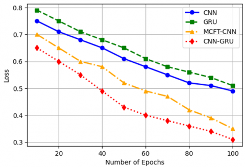
Figure 6. Loss
Figure 6 provides a valuable perspective on the loss values achieved by various models during their training phases, with a particular focus on the consistently lower loss values of the proposed CNN-GRU model compared to other models. In this context, loss measures the dissimilarity between predicted values and actual values, with lower loss values indicating more accurate predictions and better model convergence. The data presented in Figure 6 demonstrates that the CNN-GRU model consistently achieves lower loss values compared to three other models: CNN, GRU, and MCFT-CNN. Specifically, the CNN-GRU model achieves a remarkably low loss of 0.31, underscoring its outstanding performance in terms of prediction accuracy and convergence.
A loss of 0.31 for the CNN-GRU model signifies its exceptional ability to provide accurate predictions and achieve superior model convergence. This indicates that the CNN-GRU model excels in delivering precise and reliable predictions, which is crucial in the context of cross-platform malware detection. In contrast, the CNN model achieves a loss value of 0.49. The CNN's specialization in capturing spatial features may lead to less accurate predictions and slower model convergence when temporal patterns are equally crucial.
The GRU model achieves a higher loss value of 0.51, implying a larger dissimilarity between predicted and actual values compared to the CNN-GRU model. While the GRU is effective in capturing temporal patterns, its focus on sequential data may result in higher loss values and slower model convergence when spatial features are essential. Lastly, the MCFT-CNN model achieves a loss value of 0.35, confirming the CNN-GRU model's superior accuracy and convergence in terms of loss values. The CNN-GRU model's advantage lies in its unique ability to seamlessly capture both spatial and temporal patterns, resulting in more precise feature representations and better model convergence. The CNN-GRU model's lower loss values reflect its capability to provide more accurate and reliable predictions, enhancing its effectiveness in cross-platform malware detection and ensuring faster convergence during training.
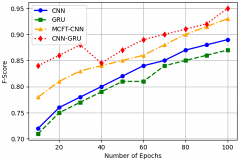
Figure 7. F-score
Figure 7 provides a comprehensive view of the F-scores achieved by various models, including the proposed CNN-GRU model, during their training phases. The F-score is a vital metric in evaluating classification models as it balances both precision and recall, providing insight into a model's ability to find a harmonious trade-off between correctly identifying malware samples and minimizing misclassifications. The F-score ranges between 0 and 1, with higher values indicating a better balance between precision and recall. The CNN-GRU model consistently achieves higher F-scores compared to three other models: CNN, GRU, and MCFT-CNN. Specifically, the CNN-GRU model achieves an F-score of 0.95, outperforming the other models.
An F-score of 0.95 for the CNN-GRU model indicates its exceptional ability to strike a balance between precision and recall, resulting in a more accurate classification performance. This means that the CNN-GRU model not only correctly identifies malware samples but also minimizes the occurrence of misclassifications or false positives and false negatives. In comparison, the CNN model achieves an F-score of 0.89, which is commendable but falls slightly short of the CNN-GRU model's performance. The CNN model's specialization in capturing spatial features may limit its capacity to achieve a more balanced trade-off between precision and recall. The GRU model achieves an F-score of 0.87, demonstrating its effectiveness in achieving a balanced classification performance. However, it still slightly trails behind the CNN-GRU model in terms of F-score. The GRU's primary focus on capturing temporal patterns may result in less optimal classification when spatial features are also crucial.
Lastly, the MCFT-CNN model achieves an F-score of 0.93, showcasing a solid performance but still not reaching the F-score attained by the CNN-GRU model. The CNN-GRU model's advantage lies in its unique ability to seamlessly capture both spatial and temporal patterns. This comprehensive approach to feature representation enables it to achieve higher F-scores, indicating a more balanced and accurate classification performance. The CNN-GRU model's capacity to excel in both precision and recall reflects its ability to maintain high accuracy while minimizing misclassifications. This balanced performance is crucial in the context of cross-platform malware detection, where both the accuracy of detection and the minimization of false alarms are critical.
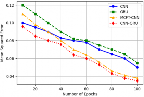
Figure 8. Mean squared error (MSE)
Figure 8 offers a valuable perspective on the Mean Squared Error (MSE) values achieved by various models, including the proposed CNN-GRU model, during their training phases. The MSE is a critical metric used to assess the accuracy of predictive models by quantifying the average of squared prediction errors. Lower MSE values indicate more accurate predictions and smaller prediction errors. The CNN-GRU model consistently achieves lower MSE values compared to three other models: CNN, GRU, and MCFT-CNN. Specifically, the CNN-GRU model achieves an impressively low MSE of 0.035, outperforming the other models.
An MSE of 0.035 for the CNN-GRU model indicates its exceptional ability to make accurate predictions with minimal prediction errors. This suggests that the CNN-GRU model excels in providing precise and reliable predictions, which is especially crucial in the context of cross-platform malware detection.
In contrast, the CNN model achieves a higher MSE of 0.050, indicating larger prediction errors compared to the CNN-GRU model. The CNN's specialization in capturing spatial features may result in less accurate predictions when temporal patterns are equally important. The GRU model achieves an MSE of 0.055, which is also higher than that of the CNN-GRU model. While the GRU is effective in capturing temporal patterns, its focus on sequential data may lead to larger prediction errors when spatial features are essential.
Lastly, the MCFT-CNN model achieves an MSE of 0.038, falling short of the CNN-GRU model's impressive accuracy in terms of prediction errors. The CNN-GRU model's advantage lies in its unique ability to seamlessly capture both spatial and temporal patterns. This comprehensive approach to feature representation results in more precise representations of malware behavior and minimizes prediction discrepancies. The CNN-GRU model's lower MSE values reflect its capability to provide more accurate and reliable predictions, making it a highly effective solution for cross-platform malware detection.
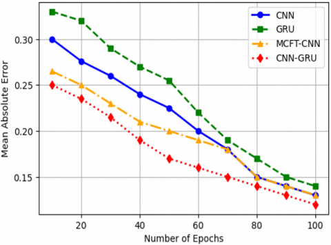
Figure 9. Mean absolute error (MAE)
Figure 9 offers valuable insight into the Mean Absolute Error (MAE) values achieved by various models, including the proposed CNN-GRU model, during their training phases. MAE is a crucial metric used to assess the accuracy of predictive models by quantifying the average of absolute prediction errors. Lower MAE values indicate more accurate predictions and smaller absolute prediction errors. The CNN-GRU model consistently achieves lower MAE values compared to three other models: CNN, GRU, and MCFT-CNN. Specifically, the CNN-GRU model achieves a remarkably low MAE of 0.12, outperforming the other models.
An MAE of 0.12 for the CNN-GRU model signifies its exceptional ability to make accurate predictions with minimal absolute prediction errors. This suggests that the CNN-GRU model excels in providing precise and reliable predictions, a critical aspect of cross-platform malware classification. In contrast, the CNN model achieves a higher MAE of 0.13, indicating larger absolute prediction errors compared to the CNN-GRU model. The CNN's specialization in capturing spatial features may result in less accurate predictions when temporal patterns are equally important.
The GRU model achieves an MAE of 0.14, which is also higher than that of the CNN-GRU model. While the GRU is effective in capturing temporal patterns, its focus on sequential data may lead to larger absolute prediction errors when spatial features are essential. Lastly, the MCFT-CNN model achieves an MAE of 0.13, further confirming the CNN-GRU model's superior accuracy in terms of absolute prediction errors. The CNN-GRU model's advantage lies in its unique ability to seamlessly capture both spatial and temporal patterns. This comprehensive approach to feature representation results in more precise representations of malware behavior and minimizes absolute prediction discrepancies. The CNN-GRU model's lower MAE values reflect its capability to provide more accurate and reliable predictions, enhancing its effectiveness in cross-platform malware classification.
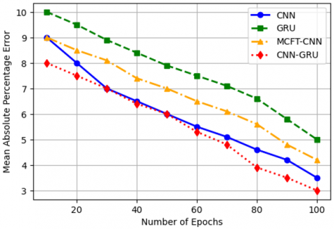
Figure 10. Mean absolute percentage error (MAPE)
Figure 10 provides valuable insight into the Mean Absolute Percentage Error (MAPE) values achieved by various models, with a special emphasis on the consistently lower MAPE values of the proposed CNN-GRU model compared to other models. MAPE is a critical metric used to assess the accuracy of predictive models by quantifying the percentage of prediction errors relative to the actual values. Smaller MAPE values indicate more accurate predictions with lower percentage prediction errors. CNN-GRU model consistently achieves lower MAPE values compared to three other models: CNN, GRU, and MCFT-CNN. Specifically, at epoch 100, the CNN-GRU model achieves a remarkably low MAPE of 3%, showcasing its outstanding performance in terms of prediction accuracy.
A MAPE of 3% for the CNN-GRU model reflects its exceptional ability to provide accurate predictions with minimal percentage prediction errors. This indicates that the CNN-GRU model excels in delivering precise and reliable predictions, which is of utmost importance in the context of cross-platform malware detection.
In contrast, the CNN model achieves a higher MAPE of 3.5%, implying a larger percentage of prediction errors compared to the CNN-GRU model. The CNN's specialization in capturing spatial features may lead to less accurate predictions when temporal patterns are equally crucial. The GRU model achieves a MAPE of 5%, which is also higher than that of the CNN-GRU model. While the GRU is effective in capturing temporal patterns, its focus on sequential data may result in a larger percentage of prediction errors when spatial features are essential. Lastly, the MCFT-CNN model achieves a MAPE of 4.2%, further confirming the CNN-GRU model's superior accuracy in terms of percentage prediction errors. The CNN-GRU model's advantage lies in its unique ability to seamlessly capture both spatial and temporal patterns. This comprehensive approach to feature representation results in more precise representations of malware behavior and minimizes percentage prediction discrepancies. The CNN-GRU model's lower MAPE values reflect its capability to provide more accurate and reliable predictions, enhancing its effectiveness in cross-platform malware detection.
Malware attacks pose a significant and growing threat in today's digital landscape, targeting multiple operating systems with increasingly sophisticated tactics. Detecting and classifying malware that can operate across diverse platforms has become a critical challenge for cybersecurity. In response to this challenge, this part of the work introduces a pioneering deep learning-based approach, known as the CNN-GRU model, designed for cross-platform malware classification. This model effectively harnesses both static and dynamic features to capture the distinct characteristics of malware behavior on platforms such as Windows, macOS, Android, and iOS. Traditional methods of malware classification often fall short in the face of evolving malware threats. These methods typically rely on either static or dynamic features, which alone may not provide a comprehensive understanding of contemporary malware's multifaceted nature. The CNN-GRU model presented in our study seeks to overcome these limitations by combining the strengths of CNN and GRU networks. This fusion allows the model to detect both spatial and temporal patterns within malware samples, thereby enhancing its accuracy and robustness.
The experimental results of our study validate the efficacy of the CNN-GRU model. It achieves an impressive accuracy rate of 93%, outperforming traditional methods by a significant margin. This high level of accuracy is a testament to the model's ability to adapt to the complexities of cross-platform malware detection. By successfully integrating static and dynamic features, the CNN-GRU model creates a comprehensive feature representation of malware behavior that enables it to excel in the face of sophisticated threats. The CNN-GRU model's cross-platform capabilities are a key feature that sets it apart from conventional methods. It can effectively classify malware on a wide range of operating systems, making it a versatile tool in the fight against malware attacks that target multiple platforms. This adaptability is crucial in today's digital landscape, where cyber threats are no longer confined to a single operating system.
One of the primary advantages of the CNN-GRU model is its ability to provide cybersecurity professionals with early detection and mitigation capabilities. With an accuracy rate of 93%, it can swiftly identify malicious software, enabling rapid response and containment of security risks. This proactive approach is vital in safeguarding critical systems and sensitive data from the ever-evolving landscape of malware threats.
[1] Felt, A.P., Finifter, M., Chin, E., Hanna, S., Wagner, D. (2011). A survey of mobile malware in the wild. In Proceedings of the 1st ACM workshop on Security and Privacy in Smartphones and Mobile Devices, pp. 3-14. https://doi.org/10.1145/2046614.2046618
[2] Tam, K., Feizollah, A., Anuar, N.B., Salleh, R., Cavallaro, L. (2017). The evolution of android malware and android analysis techniques. ACM Computing Surveys, 49(4): 1-41. https://doi.org/10.1145/3017427
[3] Ma, Z., Ge, H., Liu, Y., Zhao, M., Ma, J. (2019). A combination method for android malware detection based on control flow graphs and machine learning algorithms. IEEE Access, 7: 21235-21245. https://doi.org/10.1109/ACCESS.2019.2896003
[4] Ou, F., Xu, J. (2022). S3feature: A static sensitive subgraph-based feature for android malware detection. Computers & Security, 112: 102513. https://doi.org/10.1016/j.cose.2021.102513
[5] Karbab, E.B., Debbabi, M. (2019). Maldy: Portable, data-driven malware detection using natural language processing and machine learning techniques on behavioral analysis reports. Digital Investigation, 28: S77-S87. https://doi.org/10.1016/j.diin.2019.01.017
[6] Zhang, M., Duan, Y., Yin, H., Zhao, Z. (2014). Semantics-aware android malware classification using weighted contextual API dependency graphs. In Proceedings of the 2014 ACM SIGSAC Conference on Computer and Communications Security, New York, United States, pp. 1105-1116. https://doi.org/10.1145/2660267.2660359
[7] Vu, D.L., Nguyen, T.K., Nguyen, T.V., Nguyen, T.N., Massacci, F., Phung, P.H. (2020). Hit4mal: Hybrid image transformation for malware classification. Transactions on Emerging Telecommunications Technologies, 31(11): e3789. https://doi.org/10.1002/ett.3789
[8] Milosevic, N., Dehghantanha, A., Choo, K.K.R. (2017). Machine learning aided android malware classification. Computers & Electrical Engineering, 61: 266-274. https://doi.org/10.1016/j.compeleceng.2017.02.013
[9] Egele, M., Scholte, T., Kirda, E., Kruegel, C. (2008). A survey on automated dynamic malware-analysis techniques and tools. ACM Computing Surveys, 44(2): 1-42. https://doi.org/10.1145/2089125.2089126
[10] Wang, P., Wang, Y.S. (2015). Malware behavioural detection and vaccine development by using a support vector model classifier. Journal of Computer and System Sciences, 81(6): 1012-1026. https://doi.org/10.1016/j.jcss.2014.12.014
[11] Wang, W., Zhao, M.C., Gao, Z.Z., Xu, G.Q., Xian, H.Q., Li, Y.Y., Zhang, X.L. (2019). Constructing features for detecting android malicious applications: issues, taxonomy and directions. IEEE Access, 7: 67602-67631. https://doi.org/10.1109/ACCESS.2019.2918139
[12] Abusitta, A., Li, MQ., Fung, B.C. (2021). Malware classification and composition analysis: A survey of recent developments. Journal of Information Security and Applications, 59: 102828. https://doi.org/10.1016/j.jisa.2021.102828
[13] Mahindru, A., Singh, P. (2017). Dynamic permissions based android malware detection using machine learning techniques. In Proceedings of the 10th Innovations in Software Engineering Conference, Jaipur, India, pp. 202-210. https://doi.org/10.1145/3021460.3021485
[14] Alasmary, H., Abusnaina, A., Jang, R., Abuhamad, M., Anwar, A., Nyang, D., Mohaisen, D. (2020). Soteria: Detecting adversarial examples in control flow graph-based malware classifiers. In 2020 IEEE 40th International Conference on Distributed Computing Systems (ICDCS), Singapore, Singapore, pp. 888-898. https://doi.org/10.1109/ICDCS47774.2020.00089
[15] Arslan, R.S., Tasyurek, M. (2022). AMD-CNN: Android malware detection via feature graph and convolutional neural networks. Concurrency and Computation Practice and Experience, 34(23): e7180. https://doi.org/10.1002/cpe.7180
[16] Kumar, S., Janet, B., Neelakantan, S. (2022). Identification of malware families using stacking of textural features and machine learning. Expert Systems with Applications, 208: 118073. https://doi.org/10.1016/j.eswa.2022.118073
[17] Frenklach, T., Cohen, D., Shabtai, A., Puzis, R. (2021). Android malware detection via an app similarity graph. Computers & Security, 109: 102386. https://doi.org/10.1016/j.cose.2021.102386
[18] Nguyen, H.T., Ngo, Q.D., Le, V.H. (2020). A novel graph-based approach for IoT botnet detection. International Journal of Information Security, 19(5): 567-577. https://doi.org/10.1007/s10207-019-00475-6
[19] Pektaş, A., Acarman, T. (2020). Deep learning for effective android malware detection using API call graph embeddings. Soft Computing, 24: 1027-1043. https://doi.org/10.1007/s00500-019-03940-5
[20] Kumar, S., Janet, B. (2022). DTMIC: Deep transfer learning for malware image classification. Journal of Information Security and Applications, 64: 103063. https://doi.org/10.1016/j.jisa.2021.103063
[21] Gonzalez, H., Kadir, A.A., Stakhanova, N., Alzahrani, A.J., Ghorbani, A.A. (2015). Exploring reverse engineering symptoms in android apps. In Proceedings of the Eighth European Workshop on System Security, pp. 1-7. https://doi.org/10.1145/2751323.2751330
[22] Ullah, F., Naeem, M.R., Mostarda, L., Shah, S.A. (2021). Clone detection in 5g-enabled social IoT system using graph semantics and deep learning model. International Journal of Machine Learning and Cybernetics, 12: 3115-3127. https://doi.org/10.1007/s13042-020-01246-9
[23] Yan, J., Yan, G., Jin, D. (2019). Classifying malware represented as control flow graphs using deep graph convolutional neural network. In 2019 49th Annual IEEE/IFIP International Conference on Dependable Systems and Networks (DSN), Portland, OR, USA, pp. 52-63. https://doi.org/10.1109/DSN.2019.00020
[24] Gao, Z., Feng, A., Song, X., Wu, X. (2019). Target-dependent sentiment classification with BERT. IEEE Access, 7: 154290-154299. https://doi.org/10.1109/ACCESS.2019.2946594
[25] Oak, R., Du, M., Yan, D., Takawale, H., Amit, I. (2019). Malware detection on highly imbalanced data through sequence modeling. In Proceedings of the 12th ACM Workshop on Artificial Intelligence and Security, New York, United States, pp. 37-48. https://doi.org/10.1145/3338501.3357374
[26] Gálvez-López, D., Tardos, J.D. (2012). Bags of binary words for fast place recognition in image sequences. IEEE Transactions on Robotics, 28(5): 1188-1197. https://doi.org/10.1109/TRO.2012.2197158
[27] Ullah, F., Ullah, S., Naeem, M.R., Mostarda, L., Rho, S., Cheng, X. (2022). Cyber-threat detection system using a hybrid approach of transfer learning and multi-model image representation. Sensors, 22(15): 5883. https://doi.org/10.3390/s22155883
[28] Lee, W.Y., Saxe, J., Harang, R. (2019). SeqDroid: Obfuscated android malware detection using stacked convolutional and recurrent neural networks. Deep Learning Applications for Cyber Security, Advanced Sciences and Technologies for Security Applications, Springer, Cham, 197-210. https://doi.org/10.1007/978-3-030-13057-2_9
[29] Yerima, S.Y., Sezer, S. (2018). Droidfusion: A novel multilevel classifier fusion approach for android malware detection. IEEE Transactions on Cybernetics, 49(2): 453-466. https://doi.org/10.1109/TCYB.2017.2777960
[30] Jonsson, L., Borg, M., Broman, D., Sandahl, K., Eldh, S., Runeson, P. (2016). Automated bug assignment: Ensemble-based machine learning in large scale industrial contexts. Empirical Software Engineering, 21: 1533-1578. https://doi.org/10.1007/s10664-015-9401-9
[31] Taheri, L., Kadir, A.F.A., Lashkari, A.H. (2019). Extensible android malware detection and family classification using network-flows and API-calls. In 2019 International Carnahan Conference on Security Technology (ICCST), Chennai, India, pp. 1-8. https://doi.org/10.1109/CCST.2019.8888430
[32] Wang, A., Gao, X.D. (2021). A variable scale case-based reasoning method for evidence location in digital forensics. Future Generation Computer Systems, 122: 209-219. https://doi.org/10.1016/j.future.2021.03.019
[33] Arepalli, P.G., Naik, K.J. (2024). Water contamination analysis in IoT enabled aquaculture using deep learning based AODEGRU. Ecological Informatics, 79: 102405. https://doi.org/10.1016/j.ecoinf.2023.102405
[34] Gopi, A.P., Gowthami, M., Srujana, T., Padmini, S.G., Malleswari, M.D. (2022). Classification of denial-of-service attacks in IoT networks using AlexNet. In Human-Centric Smart Computing, Springer, Singapore, pp. 349-357. https://doi.org/10.1007/978-981-19-5403-0_30