Maimonul Karim Chowdhury*![]() | Md. Moniruzzaman Bhuyan
| Md. Moniruzzaman Bhuyan![]() | Mashky Chowdhury Surja
| Mashky Chowdhury Surja![]() | Dilara Dilshad
| Dilara Dilshad![]() | Simul Acherjee
| Simul Acherjee![]() | Ujjwal Kumar Deb
| Ujjwal Kumar Deb![]()
© 2025 The authors. This article is published by IIETA and is licensed under the CC BY 4.0 license (http://creativecommons.org/licenses/by/4.0/).
OPEN ACCESS
This numerical study emphasizes on the design of a heat exchanger by employing different geometrical configurations to improve heat transfer efficiency. This simulation employs a k-ω turbulence model with a constant temperature, by using water as the working fluid, and maintaining a Reynolds number ranging from 5,000 to 25,000. The analysis evaluates the temperature distribution, velocity distribution, pressure distribution, Nusselt number, friction factor, thermal performance evaluation, effectiveness, and vorticity magnitude. The outlet temperatures decrease as the number of inserts increases, with the maximum temperature obtained for twisted inserts for any Reynolds number studied. The highest outlet velocity is obtained without insert and lowest is for a twisted tape insert, indicating a significant reduction due to inserts. The Nusselt number remains fairly constant for all cases, only slightly increasing for the twisted-tape insert. The Performance Evaluation Criterion remains mostly constant across the Reynolds number studied, with higher values obtained for twisted-tape inserts compared to other models.
circular pipe, rectangular inserts, twisted tape inserts, simulation, heat transfer
Heat is transferred between fluids and solids of different temperatures using a heat transfer device. The enhancement of heat transfer depends on a number of factors, including fluid characteristics, insert types, and geometrical shape. High-efficiency heat exchangers are therefore crucial components of automobiles, air conditioners, refrigeration systems, the process and petrochemical industries, chemical reactor power plants, etc. In this context, researchers need to use a variety of methods and techniques to create a system that is both a suitable size and cost [1-5].
A choice of geometrical variations and inserts has been applied to enhance heat exchanger performance by increasing the turbulence and mixing of the fluid [6-11]. The effects of the inserts on smooth tubes have been explored in different studies by using spiral coil [12], twisted tapes [13], helical screw-tape inserts [14], triangle cross-sectioned coiled wire inserts [15], typical insert [16, 17], helical screw-tape inserts [18] clockwise and counter-clockwise [19], insert containing centre wings and alternate-axes [20], perforated [21] , also full and short-length inserts [22, 23].
Salam et al. [24] focused on heat transfer increase with a rectangular-cut twisted tape insert in a circular tube and examined the heat transfer coefficient, friction factor, and efficiency of turbulent water flow. A 26.6 mm inner diameter copper tube with a 5.25 twist ratio insert was tested in a uniform heat flux. Nusselt numbers increased 2.3-2.9 times, while friction factors increased 1.4-1.8 times as compared to a smooth tube. Heat transfer efficiency ranged from 1.9 to 2.3 and increased with Reynolds number.
Meyer and Abolarin [25] explored heat transfer and pressure drop for transitional flow in a circular tube using twisted tape inserts and a square-edge inlet and discovered that the Colburn j-factor varies with twisted ratios.
Acherjee et al. [26] applied numerical analysis to investigate heat transmission in a circular pipe with a perforated axial insert at multiple angles (0°-70°) during non-isothermal laminar flow. They used uniform heat flux to measure temperature and pressure distributions. Their findings show a reverse correlation between heat transfer rate and wall temperature, along with analyses of the Nusselt number, friction factor, and PEC.
Kumar et al. [27] implemented a triangular perforated twisted tape with V-cuts (TPTTV) in a double-pipe heat exchanger to increase turbulence and heat transmission. They found that numerical studies of laminar to turbulent flow showed a 50 mm pitch provided the optimum thermal-hydraulic performance, with a thermal performance factor of 1.49, exceeding plain twisted tape inserts.
Marzouk et al. [28] investigated a unique fractal tube structure in a helically coiled heat exchanger and discovered that it is more efficient than the typical design. The fractal tube heat exchanger (FTHE) provides a 289% better total heat transfer coefficient, and its exergy efficiency increased with Reynolds number, exceeding the typical helical coiled heat exchanger (HTHE).
Poblador-Ibanez et al. [29] investigated vorticity dynamics during transcritical liquid jet breakup. They explored vortical structures, vortex generating mechanisms, and the functions of hairpin and roller vortices in liquid sheet deformation. At high pressures, increased mixing and gas dissolution change liquid structures, distinguishing breakup from subcritical atomization. Near the interface, liquid density decreases by 10% and viscosity by 70%, increasing sensitivity to vortical motion.
Khaled and Mushatet [30] studied a twisted elliptical double-tube heat exchanger with ANSYS Fluent 23.1. With twisting ratios of 5 tube and 4 for tape and Reynolds numbers ranging from 5000 to 25000, their research discovered that twisted tape improved fluid mixing and heat transfer. At 5000 Reynolds, the heat exchanger's efficiency increased by 75%.
There are significant effects of multi-spring wires on the hydrothermal performance of a double tube heat exchanger. According to Sharaf et al. [31], using steel spring wires (2 mm diameter, 1000 mm length) in 1-, 2-, and 3-spring configurations provides a constant Nusselt number increase. They investigate the friction factor, Nusselt number, and energy efficiency for Reynolds numbers from 4500 to 7500. The 3-wire configuration increases Nusselt number by 112% and friction factor by 134% over plain tubes, while energy efficiency increases by 61%.
In another study, Sharaf et al. [32] studied heat transfer in a double-pipe helical heat exchanger with spring wire inserts (SWI) and nanofluids. SWI with 0.3% nanofluid enhanced the Nusselt number by 174%, reduced pressure by 157%, and improved energy efficiency by 65%. In their experiment, SWI showed better thermal-hydraulic performance than nanofluids.
Nashee et al. [33] tested numerical methods to investigate heat transmission and friction in a channel with two rows of asymmetrical obstacles. Simulations were carried out using ANSYS FLUENT 21 at Reynolds numbers ranging from 500 to 2500, with a consistent heat flow. Triangular barriers had the most heat transfer, but also the greatest pressure drop and friction factor.
In another study, Nashee [34] examined heat flow and friction in a channel with asymmetrical barriers using Ansys Fluent (k-ε model). The study explored single-cut and double-cut twisted tapes with cut ratios ranging from 0.3 to 0.9 in turbulent water flow (Re = 5000 to 25000). The results showed that double-cut tapes had better heat transmission and more friction than single-cut tapes, with thermal performance improving as the cut ratio increased.
Kadbhane and Pangavhane [35] researched heat transfer in a heat pipe using hexagonal perforated twisted tape inserts of various cut orientations. They used a hybrid deep neural network with a gannet optimization algorithm (DNN-GOA) to estimate heat transfer performance. Their experimental results reveal that alternating cuts improve convective heat transmission, and the DNN-GOA model had the highest predicted accuracy with the least errors, indicating its reliability.
Marzouk et al. [36] explored heat transfer increase in a DTHX employing a 1000 mm steel nail rod insert (NRI) with 100 mm, 50 mm, and 25 mm pitches in turbulent flow (Re 3200-5700). The 25 mm pitch provides 1.9 × better heat transmissions, but also the greatest pressure drop. Energy efficiency rises at 128%, and simulations suggest that NRI-induced turbulence promotes heat transport.
Anika et al. [37] conducted a numerical analysis of heat transfer increase in a U-loop pipe with rectangular-cut twisted tape inserts. The investigation discovered the highest Nusselt number (Nu = 357.59 at Re = 17,288.05) and better friction factor when compared to plain twisted tape and plain tube. Rectangular-cut inserts received the highest thermal performance factor (1.04), indicating their effectiveness in improving heat transmission in industrial heat exchangers.
Bhuyan et al. [38] explored the effect of twist ratios on heat transport in U-shaped pipes employing circular-cut twisted-tape inserts. A numerical simulation using a k-ω turbulent model analyzed fluid flow for Reynolds numbers from 3700 to 23,650 at constant temperatures. The results showed that when the twist ratio increased the wall and bulk temperatures, Nusselt number, effectiveness, friction factor, and thermal performance decreased. Vorticity was consistent without inserts but became erratic at cut positions with inserts. The twist ratio of three inserts significantly improved friction (5.01-5.96 times) and efficacy (1.88 times) when compared to no insert, improving thermal performance by 1.31-1.92 times.
The existing literature indicates that perforated-type inserts perform better in heat exchangers than plain tubes. However, limited research has been conducted on the impacts of rectangular-cut twisted tape inserts. The purpose of this study is to investigate the effects of multiple inserts on heat transfer and fluid flow in non-isothermal turbulent flow with water as the working fluid. The simulation results are compared to plain tubes, tubes with rectangular inserts, twisted inserts to analyze the effect of inserts on heat exchanger performance and the enhancement of heat transfer.
Computational Fluid Dynamics (CFD) is considered the most reliable tool for evaluating fluid dynamical performance within tubular pipe in a variety of applications. CFD uses computational and numerical techniques to solve Navier-Stokes equations for fluid flow inside tubes, with the mesh produced using the Finite Element Method (FEM) [39]. As CFD is based on continuity, momentum and energy, the fundamental governing equations are below [40]:
$\frac{\partial \rho}{\partial t}+\nabla \cdot(\rho \boldsymbol{u})=0$ (1)
$\begin{gathered}\rho(\boldsymbol{u} \cdot \nabla) \boldsymbol{u}=\nabla \cdot\left[-p I+\left(\mu+\mu_T\right)\left(\nabla \boldsymbol{u}+(\nabla \boldsymbol{u})^T\right)\right. \left.-\frac{2}{3}\left(\mu+\mu_T\right)(\nabla \cdot \boldsymbol{u}) I-\frac{2}{3} \rho K I\right]+F\end{gathered}$ (2)
Menter [41] formed the k-ω turbulence model, which is responsible for the turbulent kinetic energy (k) and specific dissipation rate (ω) of fluids. The CFD Module implements Wilcox’s improved k-ω model [42].
$\rho(\boldsymbol{u} \cdot \nabla) k=\nabla \cdot\left[\left(\mu+\mu_T \sigma_k^*\right) \nabla_K\right]+p_k-\rho \beta^* k \omega$ (3)
$\rho(\boldsymbol{u} \cdot \nabla) \omega=\nabla \cdot\left[\left(\mu+\mu_T \sigma_\omega\right) \nabla \omega\right]+\alpha \frac{\omega}{k} P_k-\rho \beta \omega^2$ (4)
In this concept, $\omega$ denotes the inverse time scale associated with turbulent flow. The k-ω model encompasses the advantage of being applicable to the entire boundary layer without making additional modifications. The turbulent viscosity (μT) can be obtained from:
$\rho(\boldsymbol{u} \cdot \nabla) \omega=\nabla \cdot\left[\left(\mu+\mu_T \sigma_\omega\right) \nabla \omega\right]+\alpha \frac{\omega}{k} P_k-\rho \beta \omega^2$ (5)
$\mu_T=\rho \frac{T}{\omega}$ (6)
$P_k=\mu_T\left[\nabla \boldsymbol{u}:(\nabla \boldsymbol{u})+(\nabla \boldsymbol{u})^T-\frac{2}{3}(\nabla \cdot \boldsymbol{u})^2\right]-\frac{2}{3} \rho k \nabla \cdot \boldsymbol{u}$ (7)
The equation regarding energy functions as follows:
$\rho C_p \frac{\partial T}{\partial t}+\rho C_p \boldsymbol{u} \cdot \nabla T=\nabla \cdot(k \nabla T)+Q$ (8)
Considering the fluid to be primarily at rest (i.e., u = 0), the following equation can be stated thereby:
$\rho C_p \frac{\partial T}{\partial t}+\nabla \cdot(-k \nabla T)=Q$ (9)
When the fluid is initially stationary, the convective heat transfer coefficient (h), can be computed as follows:
$h=\frac{Q}{T_w-T_h}$ (10)
Bhuiya et al. [43] measured the insert’s efficiency in the tube using the following formula:
$\varepsilon=\frac{T_o-T_i}{T_{w a v}-T_i}$ (11)
The variables $T_o, T_i$ and $T_{w \mathrm{av}}$ denote the outlet temperature, input temperature and average wall temperature, respectively. The fluid’s Nusselt number is calculated using the equation below:
$N u=\frac{h D}{k}$ (12)
The thermal conductivity of the fluid (k) and the diameter of the cross-section of the tubular pipe (D) are represented in this equation. Bhuiya et al. [44] applied the Darcy method for calculating the fluid pressure drop (ΔP) and friction factor ($f$) from inlet to outlet.
$\Delta P=h \rho g$ (13)
Hence, using the following formula, h is the fluid’s head loss:
$h=\frac{f l u^2}{2 g D}$ (14)
Also, Eqs. (12) and (13) can be used to generate Eq. (14).
$\Delta P=\frac{l}{D} \cdot \frac{f u^2 \rho}{2}$ (15)
The thermal enhancement efficiency ($\eta$) is calculated with the following sources [44].
$\eta=1.238 \times {Re}^{0.339} \times {Pr}^{-0.3}(5.25)^{-1.33}$ (16)
2.1 Boundary conditions
The boundary conditions correspond with Wilcox's k-ω model [42], as seen below:
$u=-u_o n$ (17)
Water is utilized as the work fluid here. The water’s starting temperature is set to $T$ = 293.15.
K-T in = 293.15 K, assuming no slip wall circumstances.
$\boldsymbol{u} \cdot \boldsymbol{n}=0$ (18)
$\begin{gathered}{\left[\left(\mu+\mu_T\right)\left(\nabla \boldsymbol{u}+(\nabla \boldsymbol{u})^T\right)-\frac{2}{3}\left(\mu+\mu_T\right)(\nabla \cdot \boldsymbol{u}) I-\right.} \left.\frac{2}{3} \rho k I\right] \boldsymbol{n}=-\rho \frac{u_\tau}{\delta_w} \boldsymbol{u}_{{tan~g}}\end{gathered}$ (19)
$\boldsymbol{u}_{tan~g}=\boldsymbol{u}-(\boldsymbol{u} \cdot \boldsymbol{n}) \boldsymbol{n}$ (20)
$\nabla k \cdot \boldsymbol{n}=0, \omega=-\rho \frac{c_\mu K^2}{K_v \delta_w \mu}$ (21)
The governing equations for the tube's inner wall and the outlet domain’s wall function are shown below:
$\begin{gathered}{\left[-p I+\left(\mu+\mu_T\right)\left(\nabla \boldsymbol{u}+(\nabla \boldsymbol{u})^T\right) \downarrow\right.} \left.-\frac{2}{3}\left(\mu+\mu_T\right)(\nabla \cdot \boldsymbol{u}) I-\frac{2}{3} \rho k I\right]=-f_0 \boldsymbol{n}\end{gathered}$ (22)
The boundary of the domain is subject to stable temperature conditions, as implemented by [38]:
$T=T_o=500 K$ (23)
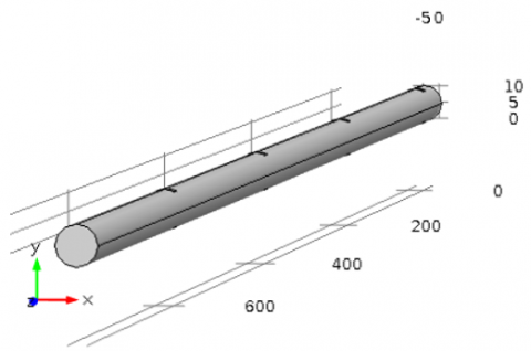
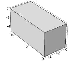
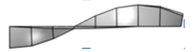
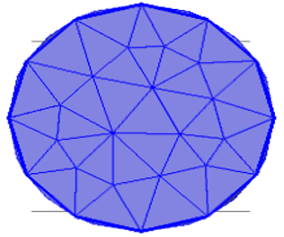
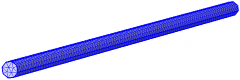
The simulation computational domain is a tubular pipe that measures 1000 mm in length, 26.6 mm in diameter, and 13.3 mm in radius shown in Figures 1(a)-(c) indicate that rectangular inserts measure 27 mm × 10 mm × 5 mm and twisted tape inserts measure 160 mm × 20 mm × 2 mm when inserted perpendicular to fluid flow inside the tube. Figures 1(d)-(e) show domain meshing as the fine mesh utilized to calculate the accuracy of the results.
(a)
(b)
(c)
(d)
(e)
Figure 1. (a) Computational full domain, (b) computational rectangular insert, (c) computational twist insert, (d) computational inlet domain of mesh design, (e) computational full-length domain of mesh design
Table 1 compares mesh designs. Since the domain is large, the results are computed with the MSI B85-PC-MATE motherboard and a computer with 16 GB of DDR3 RAM. The mesh pieces are compressed around the insert positions.
Table 1. Elements of edges
|
Name of the Property |
No Insert |
Two Inserts |
Four Inserts |
Six Inserts |
Twist Insert |
|
Element of edge |
1318 |
1340 |
1408 |
1524 |
1620 |
|
Boundary elements |
10284 |
10692 |
11246 |
11236 |
12200 |
|
No.of elements |
45,095 |
62549 |
63,630 |
60578 |
73614 |
|
Degree of freedom |
416,690 |
482,690 |
484,040 |
482285 |
483800 |
|
Volume mm3 |
1075000 |
9664000 |
9650000 |
1069000 |
9622000 |
|
Surface area mm2 |
167100 |
151600 |
136100 |
120600 |
105100 |
3.1 Simulation setup
The key objective of this simulation is to analyze the transfer of heat within a tubular pipe during non-isothermal turbulent flow. The findings of CFD analysis on water that flows across plain tubes both with and without inserts are presented in the subsequent sections. In the computation, the tube thickness is ignored, while the tube boundaries are determined utilizing the same temperature condition on the pipe’s wall. The model implements a starting velocity of 0.06 m/s to simulate turbulence an inlet temperature of 293.15 K (assuming ambient temperature), and a constant temperature condition of 500 K. As the primary goal of the numerical study is to improve the heat transfer rate of the flowing fluid, the flow through the solid tube is ignored. Simulation in the study is carried out by applying COMSOL Multiphysics. Standard parameters are used in this simulation.
In this section, results of heat transfer characteristics such as the temperature distribution, velocity distribution, pressure distribution, Nusselt number, friction factor, thermal performance evaluation, effectiveness, and vorticity magnitude for different geometric configurations are discussed.
4.1 Temperature distribution
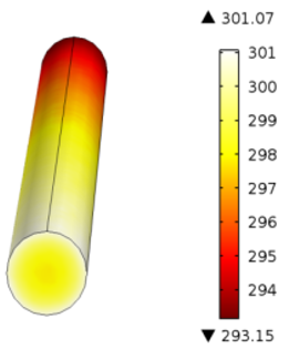
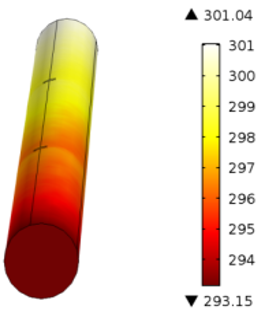
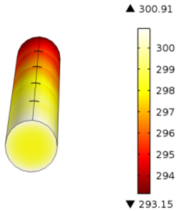
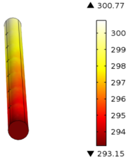
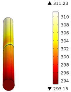
Figures 2(a)-(e) show the simulation results of temperature fluctuations for various configurations, including without an insert, two inserts, four inserts, six inserts, and a twisted tape insert. The initial temperature at the inlet is set at 293.15 K for all cases. Figure 2(a) shows the domain without an insert, with the temperature steadily increasing from 293.15 K to 301.07 K at the outlet. The temperature gradually rises through intermediate values of 294 K, 295 K, 296 K, 297 K, 298 K, 299 K, and 300 K before reaching the final outlet temperature of 301.07 K. Similarly, Figures 2(b)-(d) depict the temperature variations for domains with two, four, and six inserts. While the initial temperature remains the same at 293.15 K, the final outlet temperatures decrease slightly with an increasing number of inserts: 301.04 K for two inserts, 300.91 K for four inserts, and 300.77 K for six inserts. In contrast, Figure 2(e) illustrates the case of the twisted tape insert, where the outlet temperature reaches a significantly higher value of 311.23 K.
Figure 2. Surface temperature of the fluids for (a) no insert, (b) with two inserts, (c) with four inserts, (d) with six inserts, (e) twisted insert
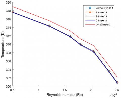
Figure 3. Change of temperature (K) with Reynolds number (Re) of the fluid
Figure 3 demonstrates the temperature variations with Reynolds number for various situations, including no insert, inserts of two, four, six, and a twisted tape insert. In all circumstances, the temperature reduces as the Reynolds number enhances. Furthermore, the results for all cases (without insert, inserts of two, four, six) are consistent, with the exception of the result with the twisted insert, which differs from the others. as the Reynolds number increases. Furthermore, the results for all cases (without insert, two inserts, four inserts, and six inserts) are consistent, with the exception of the result with the twisted insert, which differs from the others. The figure displays the temperature distributions for various domains at Reynolds numbers 12,500 and 20,033. At Reynolds number 12,500, the temperatures are 314.17 K for without insert, 314.39 K for two inserts, 314.34 K for four inserts, 314.24 K for six inserts, and 315.58 K for a twisted tape insert. In a similar manner observed at Reynolds number 20,033, the temperatures are 308.30 K for without insert, 308.42 K for two inserts, 308.31 K for four inserts, 308.16 K for six inserts, and 309.66 K for a twisted tape insert.
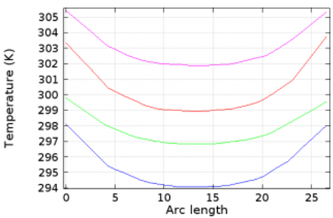
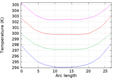
4.1.1 Cross sectional temperature distribution
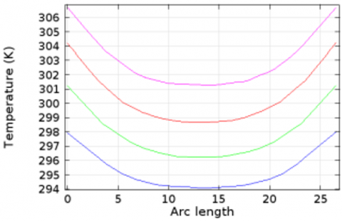
In Figure 4(a), the wall temperature is 298 K at domain position (200, 13.3, 0) to (200, -13.3, 0). And the fluid temperature the centre is gradually decreasing from wall to fluid). In the locations from (400, 13.3, 0) to (400, -13.3, 0) and (800, 13.3, 0) to (800, -13.3, 0) the fluid temperature at the centre gradually reduces more than the wall temperature. The wall temperature reaches its maximum at 800, exceeding 306 K. The fluid temperature at the center is gradually increasing. From (200, 13.3,0) to (200, -13.3, 0) position, the fluid temperature is 294 K. But it is increased to 301 K at (800, 13.3, 0) to (800, -13.3, 0) position.
Again, in Figure 4(b), the wall temperature from domain point (200, 13.3, 0) to (200, -13.3, 0) is 298 K, as in the previous figure. Similarly, the fluid temperature is lowering in its centre. The wall temperature increases when the domain positions shift from (400, 13.3, 0) to (400, -13.3, 0) and (800, 13.3, 0) to (800, -13.3, 0), but the fluid temperature decreases. The final wall temperature exceeds 305 K. The fluid temperature in the centre is progressively increasing. The fluid temperature between (200, 13.3,0) and (200, -13.3, 0) is 294 K. And it steadily increases from (800, 13.3, 0) to (800, -13.3, 0). For the inserts in Figure 4(b), the wall temperature is lower compared to Figure 4(a).
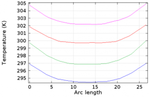
Figure 4(c) shows that the wall temperature is 298 K at domain position (200, 13.3, 0) to (200, -13.3, 0). From wall to fluid the temperature at the centre is gradually decreasing. In the locations from (400, 13.3, 0) to (400, -13.3, 0) and (800, 13.3, 0) to (800, -13.3, 0) the fluid temperature at the centre gradually decreases more than the wall temperature. The wall temperature remains its highest at 800 that is 305 K. The fluid temperature at the center is continuously increasing. From (200, 13.3,0) to (200, -13.3, 0) position, the fluid temperature is 294 K. It remains nearly 302 K at (800, 13.3, 0) to (800, -13.3, 0) position.
(a)
(b)
(c)
(d)
(e)
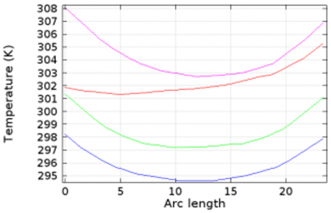
Figure 4. Cross sectional temperature line graph distribution (a) without inserts, (b) two inserts, (c) four inserts, (d) six inserts, (e) twisted tape inserts
In Figure 4(d), it can be seen that the wall temperature is 297 K at domain position (200, 13.3, 0) to (200, -13.3, 0). At the centre the fluid the temperature is reducing from wall to fluid. In the positions from (400, 13.3, 0) to (400, -13.3, 0) and (800, 13.3, 0) to (800, -13.3, 0) the fluid temperature at the centre gradually decreases more than the wall temperature similar to the previous figure. The wall temperature remains its highest at 800 mm that is 305K. The fluid temperature at the center is again increasing. From (200, 13.3,0) to (200, -13.3, 0) position, the fluid temperature is 295 K. It becomes 302 K at (800, 13.3, 0) to (800, -13.3, 0) position.
In Figure 4(e), the wall temperature is 298 K at domain position (200, 13.3, 0) to (200, -13.3, 0) which is more than all figures. At the centre the fluid the temperature is reducing from wall to fluid. In the location from (400, 13.3, 0) to (400, -13.3, 0), (600, 13.3, 0) to (600, -13.3, 0) and (800, 13.3, 0) to (800, -13.3, 0) the fluid temperature at the centre gradually decreases more than the wall temperature. The highest wall temperature is from (800, 13.3, 0) to (800, -13.3, 0) position which is 308 K. The position from (600, 13.3, 0) to (600, -13.3, 0) is little bit different as its starting wall temperature is 302K but ending is more than 305 K.
4.2 Velocity distribution
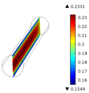
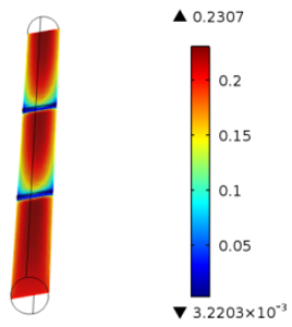
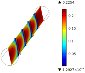
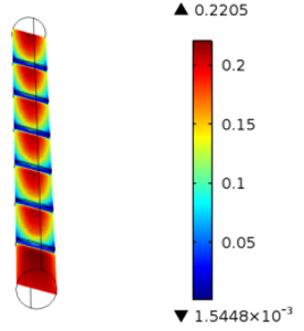
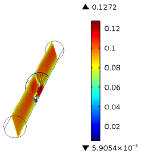
Figures 5(a)-(e) show the outlet velocity for various simulation conditions: without insert, two inserts, four inserts, six inserts, and a twisted tape insert. The outlet velocity in Figure 5(a) is 0.2331 m/sec, whereas in Figures 5(b)-(d), the velocities are 0.2307 m/sec, 0.2254 m/sec, and 0.2205 m/sec, respectively. In contrast, the outlet velocity in Figure 5(e), which depicts the twisted tape insert, is substantially lower at 0.1272 m/sec. Initially, the velocity remains the same throughout all cases, but when more inserts are included, the outlet velocity gradually decreases. The highest velocity is seen in Figure 5(a), where there is no insert, reaching 0.2331 m/sec, while the lowest outlet velocity is 0.1272 m/sec in Figure 5(e), which has a twisted tape insert. This trend suggests that the presence of inserts, specifically twisted tape, significantly reduces outlet velocity.
(a)
(b)
(c)
(d)
(e)
Figure 5. Velocity slice of the fluids for (a) no insert, (b) with two inserts, (c) with four inserts, (d) with six inserts, (e) twisted insert
4.2.1 Velocity line graph
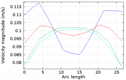
Due to the no slip condition, the velocity of pipe near the wall slightly changes in all the positions. However, velocity in the centre of the pipe increases in all positions. Figure 6(a) shows that the wall velocity from (200, 13.3, 0) to (200, -13.3, 0) is 0.074 m/sec, increased to 0.1 m/sec in the centre. The same instances occur at positions from (400, 13.3, 0) to (400, -13.3, 0), (600, 13.3, 0) to (600, -13.3, 0), and (800, 13.3, 0) to (800, -13.3, 0), where the wall velocity decreases as the central velocity steadily increases.
Again, Figure 6(b) shows that the wall velocity from (200, 13.3, 0) to (200, -13.3, 0) is 0.11 m/sec, decreased to 0.85 m/sec in the centre. There are some fluctuations for inserts. This fluctuation rate is more at (200, 13.3, 0) to (200, -13.3, 0) than (600, 13.3, 0) to (600, -13.3, 0). The same instances occur at positions from (400, 13.3, 0) to (400, -13.3, 0) and (800, 13.3, 0) to (800, -13.3, 0), where the wall velocity is increasing but the central velocity steadily decreases. Due to the inserts position this phenomenon can be seen in this figure.
(a)
(b)
(c)
(d)
(e)
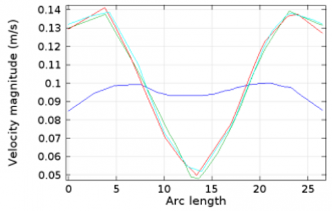
Figure 6. Velocity line of the fluids for (a) no insert, (b) with two inserts (c) with four inserts (d) with six inserts (e) twisted insert
Figure 6(c) highlights that the wall velocity from (200, 13.3, 0) to (200, -13.3, 0) is 0.8 m/sec, in the centre it becomes nearly 0.09. There are some fluctuations for inserts. This fluctuations rate is more at ((400, 13.3, 0) to (400, -13.3, 0), (600, 13.3, 0) to (600, -13.3, 0), and (800, 13.3, 0) to (800, -13.3, 0) than the position of (200, 13.3, 0) to (200, -13.3, 0). In these positions, the wall velocity is increasing but the central velocity is decreasing continuously. And the lowest velocity at center happens from (400, 13.3, 0) to (400, -13.3, 0). Due to the inserts positions this phenomenon can be seen in this figure.
Further, Figure 6(d) illustrates that the wall velocity from (200, 13.3, 0) to (200, -13.3, 0) is nearly 0.115 m/sec, in the centre it becomes nearly 0.08. There are some fluctuations for the domain being twisted. This fluctuation rate is quite similar at (400, 13.3, 0) to (400, -13.3, 0), (600, 13.3, 0) to (600, -13.3, 0), and (800, 13.3, 0) to (800, -13.3, 0). The most significant changes can be seen at the position of 600, 13.3, 0) to (600, -13.3, 0); here, the wall velocity is 0.125 m/sec but at the central it decreases to less than 0.07 m/sec which is the lowest rate among other velocities at center positions.
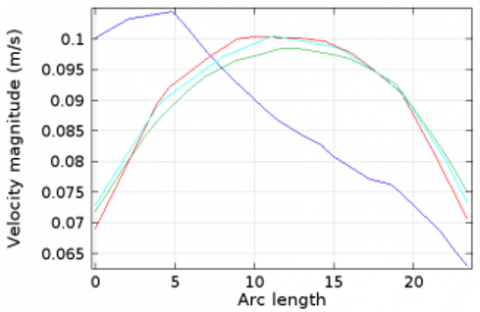
Further, Figure 6(e) illustrates that the wall velocity from (200, 13.3, 0) to (200, -13.3, 0) is nearly 0.105 m/sec, in the centre it drops sharply. There are some fluctuations for the domain being twisted. In the positions from (400, 13.3, 0) to (400, -13.3, 0), (600, 13.3, 0) to (600, -13.3, 0), and (800, 13.3, 0) to (800, -13.3, 0), where the wall velocity decreases as the central velocity steadily increases.
4.3 Pressure distribution
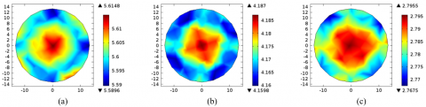
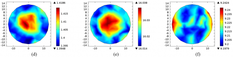
In Figures 7(a)-(d), the cross section of the pressure in the position of (200, 400, 600, 800) is decreasing from inlet to outlet. In Figure 7(a), the initial pressure is 5.5896 Pa and final pressure is 5.6148 Pa. In Figure 7(b), the initial pressure is 4.1598 Pa and it becomes 4.187 Pa finally. The same incidents happen in Figures c and d, respectively. The pressure is reducing from inlet to outlet. In Figure 7(c), at starting it is 2.7675 Pa and at end it remains 2.7955 Pa. Again, Figure 7(d) shows 1.3948 Pa at the beginning and finishes at 1.4186 Pa. And the highest initial pressure is 5.5896 Pa can show in Figure 7(a), and the lowest final pressure is at 1.4186 Pa. Therefore, there are similar scenarios that occur in all figures where the central pressure is higher in the pipe domain and comparatively lower in the wall of the pipe.
In Figures 7(e)-(h), the cross section of the pressure in the position of (200, 400, 600, 800) is reducing from inlet to outlet. In Figure 7(e), the initial pressure is 16.014 Pa and final pressure is 16.038 Pa. In Figure 7(f), the starting pressure is 9.1979 Pa and it illustrates 9.2424 Pa at the end. The same things can be seen in Figures 7(g)-(h) respectively. The pressure is lowering from inlet to outlet. In Figure 7(g), at starting it is 7.9125 Pa and at last it turns into 7.9389 Pa. Further, Figure 7(h) shows 1.4542 Pa at the beginning and finishes at 1.4774 Pa. And the highest initial pressure is 16.014 Pa that can observe in figure E and the lowest final pressure is at 1.4774 Pa. Indeed, in all figures the central pressure is higher in the pipe domain and lower in the wall of the pipe in comparison.
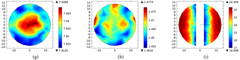
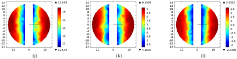
Besides, in Figures 7(i)-(l), the cross section of the pressure in the position of (200, 400, 600, 800) is also lessening from inlet to outlet. And in all figures, at the center of the inserts the domains are broken. In Figure 7(i), the initial pressure is 16.998 Pa and the ending pressure is 22.309 Pa. The initial pressure in Figure 7(j) is 10.543 Pa and it displays 15.559 Pa at the end. The pressure is lowering from inlet to outlet in Figures 7(k-l). In Figure 7(k), at the start it is 29.788 Pa and at last becomes 29.912 Pa. Similarly, Figure 7(l) shows 23.754 Pa at the beginning and at the end it is 23.792 Pa. Among these four figures of four inserts, the highest initial pressure 16.998 Pa remains in Figure 7(i) and the lowest final pressure is at 23.792 Pa remains in Figure 7(l). Indeed, in all figures the central pressure is higher in the pipe domain and lower in the wall of the pipe in comparison.
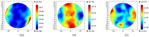
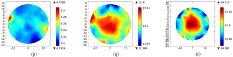
Moreover, in Figures 7(m)-(p), the cross section of the pressure in the positions of (200, 400, 600, 800) is also decreasing from inlet to outlet. Due to inserts position, there are much more pressure than the previous all figures. In Figure 7(m), the initial pressure is 29.788 Pa and the ending pressure is 29.912 Pa. The initial pressure in Figure 7(n) is 23.754 Pa and it shows 23.792 Pa at the end. The pressure is also lowering from inlet to outlet in Figures 7(m) and (p). In Figure 7(o), at starting it is 11.971 Pa and at last becomes 12.072 Pa. Likewise, Figure 7(p) shows 6.1924 Pa at the beginning and in the ending it is 6.3088 Pa. Among these four figures of six inserts, the highest initial pressure 29.788 Pa remains in Figure 7(m) and the lowest final pressure is at 6.3088 Pa can see in Figure 7(p). In Figure 7(l), the central pressure is than the other figures’ central positions.
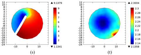
In Figures 7(q)-(t), the cross section of the pressure in the position of (200, 400, 600, 800) is also declining from inlet to outlet. Due to twisted insert position, the pressure is higher than the all the previous figures. In Figure 7(q), the initial pressure is 12.389 Pa and the ending pressure is 12.41 Pa. The initial pressure in Figure 7(r) is 10.885 Pa but it becomes 10.913 Pa at the end. The pressure is also decreasing from inlet to outlet in figures s and t. In Figure 7(s), at starting it is 1.1341 Pa and at the final, it is 9.1379 Pa. Figure 7(t) shows 2.1358 Pa at the initial point and in the final it is 2.3034 Pa.
Among these four figures of twisted inserts, the highest initial pressure can be seen at 12.389 Pa in Figure 7(m) and the lowest final pressure is 2.3034 Pa in Figure 7(p). In Figure 7(r), the central pressure is than the other figures’ central positions. And, the lowest pressure is in Figure 7(t) among all the figures (Figure 7(a-t)) because of the presence of twisted insert and the water exists from this point.
Figure 7. (a-d) no insert, (e-h) two inserts, (i-l) four inserts, (m-p) six inserts and (q-t) twisted insert
4.4 Nusselt number
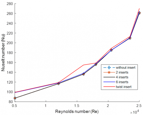
Figure 8 depicts heat transport variations as a function of Nusselt Number (Nu) and Reynolds Number (Re). The Nusselt number is found to increase with the Reynolds value in every instance of varied inserts. With a given Reynolds number, twisted tape inserts produce a greater Nusselt number than typical inserts. It also demonstrates the improved impact of twisted tape inserts on heat transfer rates. Furthermore, it is noted that the Nusselt number increases for all of the cases. This creates higher turbulent intensity and consequently gives better heat transfer. This figure demonstrates that with the Reynolds number of 12,500 the Nusselt number for all cases (without insert, inserts of two, four, six) coincide at 180. However, the twisted tape insert shows a slight increase, reaching 114.5. Again, when Reynolds number is 20,033, the Nusselt number for all cases (without insert, inserts of two, four, six) coincide at 187.3, only changes is for twisted tape insert which is 188, a little bit high. The Nusselt number result in this simulation is comparable with the experiment carried out by Salam et al. [24].
Figure 8. Change of Nusselt number (Nu) with Reynolds number (Re) of the fluid
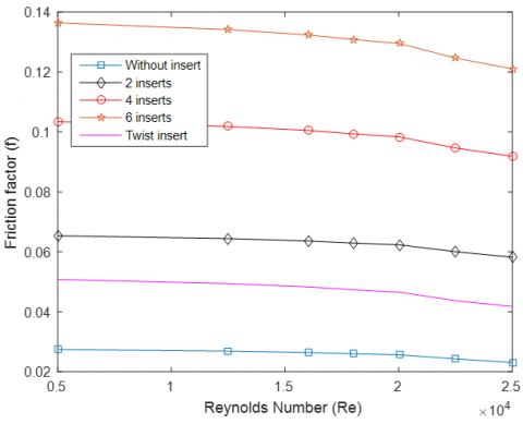
4.5 Friction factor
In this section the Reynolds number ranges from 5,000 to 25,000 for without inserts, two inserts, four inserts, six inserts, and twisted tape inserts. For all the configurations, friction factor is observed. And with the increasing of Reynolds number the friction factors are showing the decreasing pattern. At a Reynolds number of 16,030, the friction factors have been determined as 0.0264 without inserts, 0.0635 with two inserts, and 0.1005 with four inserts, 0.1323 with six inserts, and 0.0482 with twisted inserts, as seen in Figure 9. The result of friction factors in this simulation is similar to the experiment of Salam et al. [24].
Figure 9. Friction factor distributions
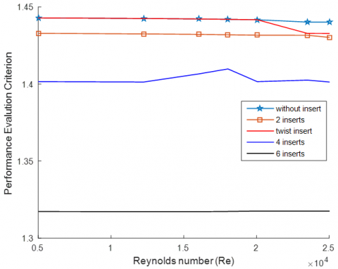
4.6 Thermal performance evaluation
Figure 10 represents thermal performance evaluation for a tube adjusted with rectangular inserts and twisted tape insert, as determined by numerical simulations. This figure shows that in comparison to the others rectangular inserts, for six inserts the performance evaluation criterion is lower. This performance evaluation criterion of four inserts is better than six inserts though there are little bit fluctuations in some places. In the context of two inserts, it shows better performance than for both four and six inserts. However, among all the situations of all inserts; the twisted tape insert performance evaluation criterion is better despite of having a small fluctuation for the higher Reynolds Number. The performance evaluation criterion for without insert is near about the twisted tape insert. This figure demonstrates that with the Reynolds number of 12,500 the Performance Evaluation Criterion for six inserts is 1.32, for 4 inserts it is 1.41, for 2 inserts it remains 1.44, for without inserts it becomes 1.443 and for twisted tape insert it shows 1.444. Besides, with the Reynolds number of 18,000 the Performance Evaluation Criterion for six inserts is 1.32, for 4 inserts where is a small fluctuation and PEC is 1.42, for 2 inserts it displays 1.44, for without insert it is 1.443 and finally for twisted tape insert is becomes 1.444. In conclusion, it can be said that the tubes fitted with twisted tape inserts give better overall heat transfer performance than the tubes without inserts, 2 inserts, 4 inserts and 6 inserts, respectively.
Figure 10. Performance evaluation criterion
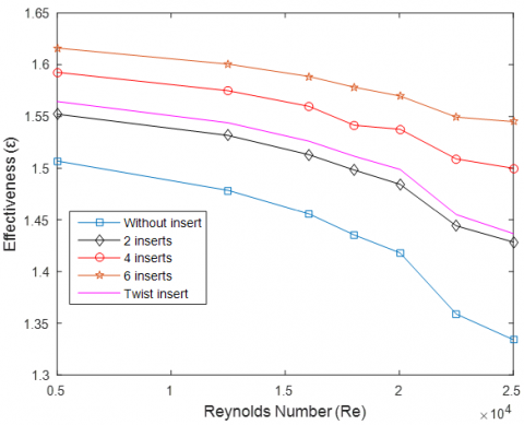
4.7 Effectiveness
In Figure 11, the Reynolds number covers from 5000 to 25,000. The figure illustrates a decreasing pattern in efficacy for all insert positions. The efficiency of the case without inserts begins at approximately 1.51 and reduces to around 1.33. A similar pattern is seen for the two-insert position. The twisted insert is more effective than the prior circumstances. The four inserts position outperforms the twisted inserts, while the six-insert position provides the best results.
Figure 11. Effectiveness distribution
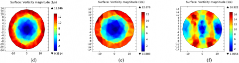
4.8 Vorticity
Figures 12(a)-(d) show the vorticity magnitude of pipe domains without inserts. Figure 12(a) depicts a 200 mm pipe domain with a fluid rotation rate of 12.358 (1/s) at the wall of domain and 0.6377 (1/s) in the centre of the pipe. Again, Figure 12(b) displays 400 mm of the pipe with a vorticity magnitude of 13.536 (1/s) near the domain wall and 0.2749 (1/s) at the centre position. Furthermore, Figure 12(c) represents 600 mm position of the pipe with a vorticity magnitude of 13.046 (1/s) near the wall and 0.3514 (1/s) in the centre. At last for the without insert for the position of 800 mm, the rotation rate is 13.046 (1/s) near the wall domain and 0.3514 (1/s) for center of the pipe in Figure 12(d). In all circumstances, the vorticity magnitude gradually increases from the center of the pipe to the domain wall.
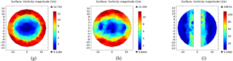
Figures 12(e)-(h) depict the vorticity magnitude of pipe domains with two inserts. Figure 12(e) shows 200 mm position of the pipe domain with a fluid rotation rate of 12.679 (1/s) near the wall of the domain and 0.1883 (1/s) in the centre of the pipe. Figure 12(f) shows 400 mm of the pipe with a vorticity magnitude of 16.922 (1/s) near the domain wall and 1.0054 (1/s) in the centre position. Furthermore, Figure 12(g) depicts 600 mm of the pipe with a vorticity magnitude of 12.716 (1/s) near the wall and 0.1189 (1/s) in the centre. Finally, for 800 mm position of the pipe, the rotation rate is 11.526 (1/s) near the wall domain and 0.8445 (1/s) at the middle of the pipe as shown in Figure 12(h). In all cases, the magnitude of the vorticity develops from the pipe’s centre line to the domain wall.
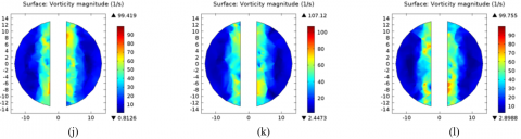
Figures 12(i)-(l) illustrate the vorticity magnitude of pipe domains with four inserts. Due to the insert position the rotation rate is more than the previous all figures. Figure 12(i) expresses 200 mm position of pipe domain with a fluid rotation rate of 108.51 (1/s) near the wall of the insert and 0.2.3383 (1/s) at the wall of the domain. Figure 12(j) shows the pipe at 400 mm with a vorticity magnitude of 99.419 (1/s) at the wall of insert and 0.8126 (1/s) at the wall of domain position. Furthermore, Figure 12(k) depicts a 600 mm of pipe with a vorticity magnitude of 107.12 (1/s) near the insert wall and 2.4473 (1/s) at the domain wall. At the end, for 800 mm position of pipe, the rotation rate is 99.755 (1/s) near the wall of insert and 2.8988 (1/s) at the wall of domain as shown in Figure 12(l). Therefore, the magnitude of the vorticity increases from the pipe’s wall to the wall of inserts in all figures. Due to the insert position, the vorticity magnitude is the maximum in all the cases of the four inserts.
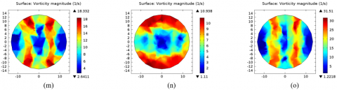
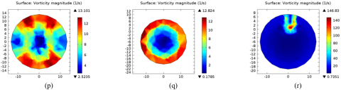
Here, Figures 12(m-p) demonstrate the vorticity magnitude of pipe domains with six inserts. Figure 12(m) shows 200 mm position of pipe domain with a fluid rotation rate of 18.332 (1/s) near the domain wall 2.6411 (1/s) in the centre of the pipe. Figure 12(n) shows a 400 mm of pipe with a vorticity magnitude of 10.938 (1/s) near the domain wall and 1.11 (1/s) in the centre position. Furthermore, Figure 12(o) depicts 600 mm of the pipe with a vorticity magnitude of 31.51(1/s) near the wall and 1.2218 (1/s) in the centre. Finally, in Figure 12(p), for 800 mm, the rotation rate is 13.101 (1/s) near the wall domain and 2.5235 (1/s) at the middle of the pipe as shown. In all cases, the magnitude of the vorticity develops from the pipe’s centre to the domain wall.
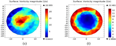
Lastly, Figures 12(q)-(t) indicate the vorticity magnitude of pipe domains with twisted tape inserts. Figure 12(q) shows the position of 200 mm pipe domain with a fluid rotation rate of 12.824 (1/s) near the domain wall 0.1785 (1/s) in the centre of the pipe. A dramatic change is observed in Figure 12(r) for twisted inserts. This figure shows 400 mm position of the pipe domain with a vorticity magnitude of 146.83 (1/s) near the domain wall and 0.7351 (1/s) in the centre position. Moreover, Figure 12(s) depicts 600 mm of the pipe with a vorticity magnitude of 22.055 (1/s) near the wall and 0.6413 (1/s) in the centre. Ultimately, in Figure 12(t), for 800 mm, the rotation rate is 12.461 (1/s) near the wall domain and 2.9906 (1/s) at the middle of the pipe as shown. All the results show that `the magnitude of the vorticity develops from the pipe’s centre to the domain wall. However, at the ending it can be said that for remaining at the insert position, the vorticity magnitude is higher in Figure 12(r) than others in the twisted insert positions.
Figure 12. Vorticity Magnitude with (a-d) no insert, (e-h) 2 inserts, (i-l) 4 inserts, (m-p) 6 inserts and (q-t) twist insert, respectively
Numerical simulations have been performed to find the effect of the number of inserts (2, 4, 6) in a tubular pipe on the temperature distribution, velocity distribution, pressure distribution, Nusselt number, friction factor, thermal performance evaluation, effectiveness, and vorticity magnitude. The results can be summarized as follows.
To summarise, the effectiveness and vorticity of the fluid improves in presence of multiple inserts, compared to the plain tube. This indicates better thermal performance of fluid flow across a tubular pipe in presence of multiple inserts. This can be used in a wide range of applications such as automobiles, air conditioners, refrigeration systems, the process and petrochemical industries, chemical reactor power plants, etc. Future research may involve inserts of different shapes and cuts.
The authors acknowledge the cordial scientific assistance of the Centre of Excellence in Mathematics (CEM), Department of Mathematics, Mahidol University, Bangkok 10400, Thailand as well as the Data Analysis and Simulation Lab, Department of Mathematics, Chittagong University of Engineering & Technology, Chittagong 4349, Bangladesh.
|
l |
Length of the pipe |
|
D |
Diameter of the pipe |
|
CP |
Specific heat, J. kg-1. K-1 |
|
$\Delta P$ |
Pressure drop |
|
g |
gravitational acceleration, m.s-2 |
|
k |
Thermal conductivity, W.m-1. K-1 |
|
f |
Friction factor(-) |
|
Nu |
Nusselt number(-) |
|
Re |
Reynolds number(-) |
|
Ti |
Inlet temperature (K) |
|
To |
Outlet temperature (K) |
|
Tb |
Bulk temperature (K) |
|
Tw |
Wall temperature (K) |
|
Twav |
Average wall temperature (K) |
|
q |
Heat flux (W/m2) |
|
Q |
Amount of heat Joule(j) |
|
Greek symbols |
|
|
µ |
Dynamic viscosity, kg. m-1.s-1 |
|
$\omega$ |
Inverse time scale |
|
$\mu_T$ |
Turbulent viscosity |
|
$\varepsilon$ |
Effectiveness |
|
$\eta$ |
Thermal enhancement performance |
|
$\rho$ |
Density of water |
[1] Webb, R.L., Kim, N.Y. (2005). Enhanced Heat Transfer. Second Edition, Taylor Francis Group.
[2] Dewan, A., Mahanta, P., Raju, K.S., Kumar, P.S. (2004). Review of passive heat transfer augmentation techniques. Proceedings of the Institution of Mechanical Engineers, Part A: Journal of Power and Energy, 218(7): 509-527. https://doi.org/10.1243/0957650042456953
[3] Eiamsa-Ard, S., Thianpong, C., Promvonge, P. (2006). Experimental investigation of heat transfer and flow friction in a circular tube fitted with regularly spaced twisted tape elements. International Communications in Heat and Mass Transfer, 33(10): 1225-1233. https://doi.org/10.1016/j.icheatmasstransfer.2006.08.002
[4] Eiamsa-Ard, S., Promvonge, P. (2007). Heat transfer characteristics in a tube fitted with helical screw-tape with/without core-rod inserts. International Communications in Heat and Mass Transfer, 34(2): 176-185. https://doi.org/10.1016/j.icheatmasstransfer.2006.10.006
[5] Eiamsa-ard, S., Pethkool, S., Thianpong, C., Promvonge, P. (2008). Turbulent flow heat transfer and pressure loss in a double pipe heat exchanger with louvered strip inserts. International Communications in Heat and Mass Transfer, 35(2): 120-129. https://doi.org/10.1016/j.icheatmasstransfer.2007.07.003
[6] Marzouk, S.A., Aljabr, A., Almehmadi, F.A., Alqaed, S., Sharaf, M.A. (2023). Numerical study of heat transfer, exergy efficiency, and friction factor with nanofluids in a plate heat exchanger. Journal of Thermal Analysis and Calorimetry, 148(20): 11269-11281. https://doi.org/10.1007/s10973-023-12441-5
[7] El-Fakharany, M.K., Abo-Samra, A.E.A., Abdelmaqsoud, A.M., Marzouk, S.A. (2024). Enhanced performance assessment of an integrated evacuated tube and flat plate collector solar air heater with thermal storage material. Applied Thermal Engineering, 243: 122653. https://doi.org/10.1016/j.applthermaleng.2024.122653
[8] Saravanan, A., Jaisankar, S. (2019). Heat transfer augmentation techniques in forced flow V-trough solar collector equipped with V-cut and square cut twisted tape. International Journal of Thermal Sciences, 140: 59-70. https://doi.org/10.1016/j.ijthermalsci.2019.02.030
[9] Lahmer, D., Benamara, N., Ahmad, H., Ameur, H., Boulenouar, A. (2022). Combination of the parallel/counter flows nanofluid techniques to improve the performances of double-tube thermal exchangers. Arabian Journal for Science and Engineering, 47: 7789-7796. https://doi.org/10.1007/s13369-022-06670-3
[10] Marzouk, S.A., Abou Al-Sood, M.M., El-Said, E.M.S., El-Fakharany, M.K. (2020). Effect of wired nails circular–rod inserts on tube side performance of shell and tube heat exchanger: Experimental study. Applied Thermal Engineering, 167: 114696. https://doi.org/10.1016/j.applthermaleng.2019.114696
[11] Bhuyan, M.M., Deb, U.K., Shahriar, M., Acherjee, S. (2017). Simulation of heat transfer in a tubular U-loop pipe using the rectangular inserts and without insert. AIP Conference Proceedings, 1851: 020011. https://doi.org/10.1063/1.4984640
[12] Mir, A., Karouei, S.H.H., Rasheed, R.H., Singh, P.K., Dixit, S., Ali, R., Aich, W., Kolsi, L. (2025). Numerical investigation of the effect of three types of spiral coils on the hydrothermal behavior of fluid flow in a shell and coil heat exchanger. Case Studies in Thermal Engineering, 70: 106078. https://doi.org/10.1016/j.csite.2025.106078
[13] Saha, S.K., Gaitonde, U.N., Date, A.W. (1989). Heat transfer and pressure drop characteristics of laminar flow in a circular tube fitted with regularly spaced twisted-tape elements. Experimental Thermal and Fluid Science, 2(3): 310-322. https://doi.org/10.1016/0894-1777(89)90020-4
[14] Sivashanmugam, P., Suresh, S. (2006). Experimental studies on heat transfer and friction factor characteristics of laminar flow through a circular tube fitted with helical screw-tape inserts. Applied Thermal Engineering, 26(16): 1990-1997. https://doi.org/10.1016/j.applthermaleng.2006.01.008
[15] Gunes, S., Ozceyhan, V., Buyukalaca, O. (2010). Heat transfer enhancement in a tube with equilateral triangle cross-sectioned coiled wire inserts. Experimental Thermal and Fluid Science, 34(6): 684-691. https://doi.org/10.1016/j.expthermflusci.2009.12.010
[16] Kumar, A., Prasad, B. (2000). Investigation of twisted tape inserted solar water heaters—Heat transfer, friction factor and thermal performance results. Renewable Energy, 19(3): 379-398. https://doi.org/10.1016/S0960-1481(99)00061-0
[17] Song, S., Liao, Q., Shen, W. (2013). Laminar heat transfer and friction characteristics of microencapsulated phase change material slurry in a circular tube with twisted tape inserts. Applied Thermal Engineering, 50(1): 791-798. https://doi.org/10.1016/j.applthermaleng.2012.07.026
[18] Ibrahim, E.Z. (2011). Augmentation of laminar flow and heat transfer in flat tubes by means of helical screw-tape inserts. Energy Conversion and Management, 52(1): 250-257. https://doi.org/10.1016/j.enconman.2010.06.065
[19] Eiamsa-ard, S., Promvonge, P. (2010). Performance assessment in a heat exchanger tube with alternate clockwise and counter-clockwise twisted-tape inserts. International Journal of Heat and Mass Transfer, 53(7-8): 1364–1372. https://doi.org/10.1016/j.ijheatmasstransfer.2009.12.023
[20] Eiamsa-ard, S., Wongcharee, K., Eiamsa-ard, P., Thianpong, C. (2010). Thermo hydraulic investigation of turbulent flow through a round tube equipped with twisted tapes consisting of centre wings and alternate-axes. Experimental Thermal and Fluid Science, 34(8): 1151-1161. https://doi.org/10.1016/j.expthermflusci.2010.04.004
[21] Thianpong, C., Eiamsa-ard, P., Promvonge, P., Eiamsa-ard, S. (2012). Effect of perforated twisted-tapes with parallel wings on heat transfer enhancement in a heat exchanger tube. Energy Procedia, 14: 1117-1123. https://doi.org/10.1016/j.egypro.2011.12.1064
[22] Bhuyan, M., Deb, U., Shahriar, M., Acherjee, S. (2017) Simulation of heat transfer in a tubular pipe using different twisted tape inserts. Open Journal of Fluid Dynamics, 7(3): 397-409. https://doi.org/10.4236/ojfd.2017.73027
[23] Eiamsa-Ard, S., Thianpong, C., Eiamsa-Ard, P., Promvonge, P. (2009). Convective heat transfer in a circular tube with short-length twisted tape insert. International Communications in Heat and Mass Transfer, 36(4): 365-371. https://doi.org/10.1016/j.icheatmasstransfer.2009.01.006
[24] Salam, B., Biswas, S., Saha, S., Bhuiya, M.M.K. (2013). Heat transfer enhancement in a tube using rectangular-cut twisted tape insert. Procedia Engineering, 56: 96-103. https://doi.org/10.1016/j.proeng.2013.03.094
[25] Meyer, J.P., Abolarin, S.M. (2018). Heat transfer and pressure drop in the transitional flow regime for a smooth circular tube with twisted tape inserts and a square-edged inlet. International Journal of Heat and Mass Transfer, 117: 11-29. https://doi.org/10.1016/j.ijheatmasstransfer.2017.09.103
[26] Acherjee, S., Deb, U.K., Bhuyan, M.M. (2019). The effect of the angle of perforation on perforated inserts in a pipe flow for heat transfer analysis. Mathematics and Computers in Simulation, 171: 306-314. https://doi.org/10.1016/j.matcom.2019.10.003
[27] Kumar, R., Nandan, G., Dwivedi, G., Shukla, A.K., Shrivastava, R. (2020). Modeling of triangular perforated twisted tape with V-cuts in double pipe heat exchanger. Materials Today: Proceedings, 46: 5389-5395. https://doi.org/10.1016/j.matpr.2020.09.038
[28] Marzouk, S.A., Abou Al-Sood, M.M., El-Said, E.M.S., Younes, M.M., El-Fakharany, M.K. (2023). Experimental and numerical investigation of a novel fractal tube configuration in helically tube heat exchanger. International Journal of Thermal Sciences, 187: 108175. https://doi.org/10.1016/j.ijthermalsci.2023.108175
[29] Poblador-Ibanez, J., Sirignano, W.A., Hussain, F. (2024). Vorticity dynamics in transcritical liquid jet breakup. Journal of Fluid Mechanics, 978: A6. https://doi.org/10.1017/jfm.2023.961
[30] Khaled, R.A., Mushatet, K.S. (2023). CFD analysis for a twisted elliptical double tube heat exchangers integrated with a twisted tape. International Journal of Heat and Technology, 41(5): 1301-1308. https://doi.org/10.18280/ijht.410520
[31] Sharaf, M.A., Marzouk, S.A., Aljabr, A., Almehmadi, F.A., Alam, T., Teklemariyem, D.A. (2024). Effects of multi-spring wires on hydrothermal performance of double tube heat exchanger. Case Studies in Thermal Engineering, 60: 104689. https://doi.org/10.1016/j.csite.2024.104689
[32] Sharaf, M.A., Marzouk, S.A., Aljabr, A., Almehmadi, F.A., Kaood, A., Alqaed, S. (2024). Heat transfer enhancement in a double-pipe helical heat exchanger using spring wire insert and nanofluid. Journal of Thermal Analysis and Calorimetry, 149: 5017-5033. https://doi.org/10.1007/s10973-024-12992-1
[33] Nashee, S.R., Ibrahim, Z.A., Kamil, D.J. (2024). Numerical investigation of flow in vertical rectangular channels equipped with three different obstacles shape. AIP Conference Proceedings, 3122: 100002. https://doi.org/10.1063/5.0216016
[34] Nashee, S.R. (2024). Numerical simulation of heat transfer enhancement of a heat exchanger tube fitted with single and double-cut twisted tapes. International Journal of Heat and Technology, 42(3): 1003-1010. https://doi.org/10.18280/ijht.420327
[35] Kadbhane, S.V., Pangavhane, D.R. (2024). Performance prediction and evaluation of heat pipe with hexagonal perforated twisted tape inserts. Heat and Mass Transfer, 60: 987-1008. https://doi.org/10.1007/s00231-024-03469-w
[36] Marzouk, S.A., Almehmadi, F.A., Aljabr, A., Sharaf, M.A. (2024). Numerical and experimental investigation of heat transfer enhancement in double tube heat exchanger using nail rod inserts. Scientific Reports, 14: 9637. https://doi.org/10.1038/s41598-024-59085-5
[37] Anika, I.O., Bhuyan, M.M., Deb, U.K. (2024). Enhancement of heat transfer in a pipe fitted with rectangular cut twisted tape inserts. International Journal of Heat and Technology, 42(5): 1501-1506. https://doi.org/10.18280/ijht.420502
[38] Bhuyan, M.M., Surja, M.C., Deb, U.K. (2024). Effect of twist ratios on heat transfer for circular-cut twisted tape inserts in U-shaped pipe. International Journal of Heat and Technology, 42(6): 1952–1962. https://doi.org/10.18280/ijht.420612
[39] Reddy, J.N. (2005). An Introduction to the Finite Element Method (Vol. 3). New York: McGraw-Hill.
[40] www.comsolmultiphysics.com, accessed on April 2025.
[41] Menter, F.R. (1994). Two-equation eddy-viscosity turbulence models for engineering applications. AIAA Journal, 32(8): 1598-1605. https://doi.org/10.2514/3.12149
[42] Wilcox, D.C. (1994). Simulation of transition with a two equation turbulence model. AIAA Journal, 32(2): 247- 255. https://doi.org/10.2514/3.59994
[43] Bhuiya, M.M.K., Ahamed, J.U., Sarkar, M.A.R., Salam, B., Sayem, A.S.M., Rahman, A. (2014). Performance of turbulent flow heat transfer through a tube with perforated strip inserts. Heat Transfer Engineering, 35(1): 43-52. https://doi.org/10.1080/01457632.2013.810449
[44] Bhuiya, M.M.K., Chowdhury, M.S.U., Islam, M., Ahamed, J.U., Khan, M.J.H., Sarker, M.R.I., Saha, M. (2012). Heat transfer performance evaluation for turbulent flow through a tube with twisted wire brush inserts. International Communications in Heat and Mass Transfer, 39(10): 1505-1512. https://doi.org/10.1016/j.icheatmasstransfer.2012.10.005