Mohammad Reza Masoumi Somarin![]() | Majid Kamvar*
| Majid Kamvar*![]() | Alireza Firoozgan
| Alireza Firoozgan![]() | Mohammad Mazidi Sharfabadi
| Mohammad Mazidi Sharfabadi![]()
© 2025 The authors. This article is published by IIETA and is licensed under the CC BY 4.0 license (http://creativecommons.org/licenses/by/4.0/).
OPEN ACCESS
Thermal management of high-temperature solid oxide fuel cells (HT-SOFCs) is very important especially in long-term applications. Anode and cathode channels geometry plays a key factor on thermal behavior of SOFCs. In this study, different schemes of gas flow cross-sectional channels are examined and compared. The study procedure is considered in two steps. First, a comparison between different rectangular cross sections gas channels with different aspect ratios is carried out and then, the scheme having less temperature gradient as a base case for second step to examine with the other two shapes including triangular and semicircular geometries in this study with the aim of improving temperature uniformity. For this purpose, the validated CFD code used for solving fully-coupled mass, continuity, momentum, charge and energy transport equations in three dimensions under steady state conditions. Results show that wider cathode channel and narrower anode channel when using rectangular electrode channels are more suitable in long-term applications. Furthermore, rectangular and triangular geometries, in comparison with the semicircular one, are preferred. Eventually, to fulfill the channel geometry effect on the cell thermal behavior, the parametric study is performed.
channel geometry, numerical modelling, planar solid oxide fuel cell, thermal management
Running out of conventional fuel resources such as fossil fuels is a challenge to supply required energy sources recently [1]. Plus, using these types of fuels rises the production of greenhouse gases and is also the most relevant reason of the observed climate change since the mid-20th century [2]. To decrease today's dependency on fossil fuels, intensive research has been conducted on the development of fuel cell systems as an alternative energy resource [3]. Among these, solid oxide fuel cells (SOFCs) as a high temperature fuel cells have received much more attention due to their special advantages such as high electrical efficiency [4]. However, this high operational temperature of SOFCs brings some challenges that need to be overcome [4]. For this purpose, research efforts have been made to reduce this operational temperature range while maintaining the cell performance high [4]. Research works in this area can be divided into two categories, experimental and numerical studies. Experimental works in these recent years have been mostly focused on the fabrication methods and new materials for SOFCs components [5-10]. Besides experimental studies provide many valuable data, but they are costly, time consuming, limited and in some cases impossible. Accessing detailed internal data such as temperature, velocity, current and molar concentration of the gaseous species throughout the cell necessitates the use of numerical tools. Especially, when minimizing thermal stresses that occur in the cell because of difference in the thermal expansion coefficient in the PEN is the target. With recent numerical studies focusing on gas flow channel design, Gong et al. [11] proposed a novel rotary L-type gas flow for SOFC showing at least 40% more uniformity index leading to better control of the thermal stress of the SOFC. Another affecting factor on thermal management of SOFCs is interconnect design. Kim et al. [12] reported a new interconnect geometry for a 1-kW planar SOFC stack and examined the effects of its design variables on internal thermal conditions via a three-dimensional thermo-fluid simulation. Their result revealed a 50℃ decrease in the vertical temperature difference. Quach et al. [13] proposed a novel interconnector design using a three-dimensional model to reduce the temperature difference by 40% in an ammonia-fueled planar SOFC stack. Another way to overcome large temperature gradients occurring in the cell is to insert an obstacle in the channels. Chellehbari et al. [14] worked on a new gas channel design with different number, cross section and size of obstacles effects on a planar SOFC performance. Their three-dimensional finite element method-based revealed that increasing the number of obstacles and considering rectangular cross section compared to trapezoid and triangular cross section, improved the cell performance. Also, flow arrangement design is the other applicable solution to improve the temperature uniformity. Kong et al. [15] worked on improving the planar SOFC performance by introducing a new design of interconnector called X-type interconnect. Their finding indicated that with the new design, the performance improved in comparison to the conventional cells. Moreno-Blanco et al. [16] analyzed the way channel-electrode interface area affects. The planar SOFC performance. They showed that channel width and numbers in a co-flow pattern directly affected the cell efficiency. In a very recent work, Aghaei et al. [17] examined the effect of gas flow channel geometry on dynamic response of a planar solid oxide fuel cell to a step difference in the cell voltage. Their study was more focused on the cell performance instead of thermal management. Furthermore, the interconnector domains were disregarded in their three-dimensional model. Wang et al. [18] reported that considering the interconnect in the numerical model was essential. While SOFCs in planar geometry compared to other types produce much more power density, they are exposed more to thermal stresses especially within PEN layers. In another recent work, Fan et al. [19] estimated the pitch width and rib width alternation of the anode and cathode channels effect on the output power density produced, temperature and concentration distributions of an anode-supported planar SOFC stack using a three-dimensional model. They found out that the cell performance can be improved by using narrower channels and this effect was more significant at cathode channels. However, they did not work on temperature gradients that occur within the cell which is very important in durability of long-term applications and non-rectangular cross-sections were not considered. Lee et al. [20] argued on the role of the distribution of temperature on the SOFCs efficiency for different channel designs in a high current density region. Three flow patterns including co-, counter- and cross-flow were compared. They claimed that the counter-flow configuration was the best scheme around high current density ranges. Although all these studies provide valuable data in controlling thermal gradients, examining the channel geometry variations (including both shapes and aspect ratios of rectangular shapes which are more common in planar type of SOFCs) in thermal management is missing.
There have been some numerical approaches in the previous studies working on thermal stresses occurring in the cell [21-26]. All these studies confirm that there is an urgency for the SOFC in planar shape to control the temperature gradient in the cell and remove the hot spot that occurs inside the cell. It is only in this situation that its long-term operation durability can be guaranteed. Therefore, the current study focuses on thermal management of a planar hydrogen-fueled anode-supported SOFC. This study is performed in two steps: step 1 involves the examination of changes in aspect ratio in rectangular cross-section of anode and cathode channels effects on temperature uniformity throughout the cell layers. Then the scheme showing the worst temperature uniformity is chosen to examine whether it can be modified by changing the cross-section or not. To have more logical comparison, all alterations take place in a constant cross-sectional area.
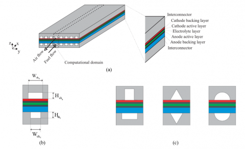
Figure 1. (a) A planar SOFC schematic with a row of the counter-flow channels (b) Aspect ratio of the different rectangular cross-sections considered in this study (c) comparison of the different shapes located as flow channels
Prediction of the thermal behavior of a single planar SOFC under steady state conditions was done using a 3D numerical model. In order to examine just shape of channel cross-sections, the fluid flow arrangement is fixed as counter-flow in all cases. The counter-flow arrangement is opted because its electric performance and temperature uniformity are better than co-flow arrangement [20, 27]. However, the gradient of temperature in the counter-flow arrangement is much higher [11]. Figure 1 depicts the schematic of the single planar SOFC with counter-flow arrangement. As shown, a row of flow channels is used to transport fuel and oxidant gaseous species toward the cell layers. Considering the geometric symmetry, the cell with only one pair of channels constructs the computational domain of this study. It involves two interconnectors, two cathode and anode backing layers, two cathode and anode active layers and electrolyte layer. In addition to these seven domains, two separate channels enable fuel and oxidant transport to the active layers. The typical materials for SOFCs noted by Zhang et al. [28] are regarded. The geometrical parameters for this model are listed in Table 1. To apply different shapes of rectangular cross-section in anode and cathode channels, the aspect ratio (AR) is defined as width-to-height ratio for each anode and cathode channel. To reduce the problem complication, the following simplifications are regarded:
• Steady state conditions.
• Flow is incompressible and laminar.
• Ideal behavior of gases and mixtures is assumed.
• Stokes-Brinkman’s assumption is applied to porous media flow.
• The thermal diffusion is disregarded.
• Thermal balance is considered among solid and fluid particles in porous media.
• The electrolyte is fully impermeable.
• Gravity effects are ignored.
Table 1. Geometrical parameters
|
Description |
Symbol |
Value |
|
Cell length Cell width Interconnectors height Anode backing layer thickness Anode active layer thickness Electrolyte thickness Thickness of cathode current collector Thickness of cathode functional layer |
Lcell Wcell Hint ta tac te tc tcc |
10 [cm] 2.5 [mm] 1.2 [mm] 400 [μm] 15 [μm] 10 [μm] 50 [μm] 20 [μm] |
With these assumptions, governing equations namely mass, momentum, charges (ion and electron) and energy coupled with the electrochemical relationships are formulated as follows:
2.1 Mass and momentum conservation
The equation of continuity for incompressible fluids is as follows [29]:
$\nabla .\left( \rho u \right)={{Q}_{m}}$ (1)
where, $\rho$ and u represent the mixture density and velocity vector, respectively. Qm is the mass source term due to electrochemical reactions. Its value is equal to zero except at active layers. In hydrogen-fueled SOFCs, two common electrochemical reactions are happened at electrode active layers [30]:
• Oxidation of hydrogen occurring at anode active layer:
${{H}_{2}}+{{O}^{-2}}\to {{H}_{2}}O+2{{e}^{-}}$ (2)
• Oxygen reduction occurring at cathode active layer:
${{O}_{2}}+2{{e}^{-}}\to {{O}^{-2}}$ (3)
Eq. (4) represents the stationary free and porous media flow transport equation for an incompressible flow using Darcy’s law [31, 32]:
$\begin{align} & \frac{\rho }{\varepsilon }\left( \left( u.\nabla \right)\frac{u}{\varepsilon } \right)= \\ & \nabla .\left( -pI+\frac{\mu }{\varepsilon }\left( \nabla \text{u}+{{\left( \nabla u \right)}^{T}} \right)-\frac{2\mu }{3\varepsilon }\left( \nabla .u \right)I \right) \\ & +\rho g-\left( \frac{\mu }{K} \right)u+F \\\end{align}$ (4)
where, µ indicates the fluid dynamic viscosity, $\kappa$ and ε represent permeability and porosity, respectively, and F shows the volume force exerted on the fluid. Using Stokes-Brinkman’s assumption in porous layers, the inertial part ((u.∇)u/ε) in porous flow is neglected. However, in channel flow, porosity ε is considered to be 1, and permeability $\kappa$ is regarded as infinite. Note that as electrolyte dense layer is sandwiched between anode and cathode sides, two separate flows are created. Also, these equations are disabled in electrolyte layer. The dynamic viscosity, μf, is calculated by [33].
${{\mu }_{f}}=\underset{j}{\mathop \sum }\,{{x}_{j}}{{\mu }_{j}}$ (5)
where, μj represents the dynamic viscosity of the jth species and xj indicates its mole fraction.
2.2 Species transport
The equation of species transport for each species is [34]:
$\nabla .{{j}_{i}}+\rho \left( u.\nabla \right){{\omega }_{i}}={{R}_{i}}$ (6)
where, ji and ωi show the relative mass flux vector and the mass fraction of the ith species, respectively, and Ri indicates the source term representing the mass consumption or production of the ith species. Using the Maxwell-Stefan diffusion model, we have [35]:
${{j}_{i}}=-\rho {{\omega }_{i}}\underset{k}{\mathop \sum }\,{{D}_{ik}}{{d}_{k}}$ (7)
where, Dik and dk refer to the multicomponent Fick’s diffusivities and the diffusional driving force, respectively, which is the former can be obtained in m2/s using Fueller, Schettler and Giddings relation [36].
$\begin{align} & {{D}_{ik}}=1.013\times \\ & {{10}^{-2}}{{T}^{1.75}}{{\left( \frac{1}{{{M}_{i}}}+\frac{1}{{{M}_{k}}} \right)}^{{}^{1}/{}_{2}}}/\left( p{{\left( v_{i}^{{}^{1}/{}_{2}}+v_{k}^{{}^{1}/{}_{2}} \right)}^{2}} \right) \\\end{align}$ (8)
where, T and p are the absolute temperature and pressure in K and Pa, respectively, Mi is the molecular weight in g/mol and νi is the molecular diffusion volume in cm3/mol. The values of νi for different species are tabulated by Taylor and Krishna [34]. The multicomponent Fick’s diffusivities are modified to take resistance to mass transfer in electrodes into account [37].
$D_{ik}^{eff}=\left( {}^{\varepsilon }/{}_{\tau } \right){{D}_{ik}}$ (9)
where, τ represents the tortuosity.
2.3 Charge conservation
Based on Ohm’s law, ion and electron conservation equations are formulated as [38]:
$-\nabla .\left( {{\sigma }_{e}}\nabla {{\phi }_{e}} \right)={{j}_{e}}$ (10)
$-\nabla .\left( {{\sigma }_{i}}\nabla {{\phi }_{i}} \right)={{j}_{i}}$ (11)
where, Φe and Φirefer to the electric and ionic potential and σe and σi refer to the electronic and ionic conductivity, respectively. For obtaining electronic and ionic conductivity in electrodes, the porous structural dependency factors should be accounted. For this, readers are referred to the studies of Andersson et al. [39, 40].
je and ji in Eqs. (10) and (11) represent electrical and ionic charge sink or source terms, respectively, which are limited to the cathode and anode catalyst layers. According to electrochemical equations occurring within the cell, electrons and ions are generated in the anode and cathode, respectively. In this study, the activation-controlled Butler-Volmer equation is used for electrochemical relationship modelling [41].
${{j}_{i.a}}=-{{j}_{e.a}}={{A}_{a}}{{j}_{0.a}}\left[ \begin{align} & exp\left( n{{\alpha }_{a}}F{{\eta }_{act.a}}/{{R}_{u}}T \right) \\ & -exp\left( -n\left( 1-{{\alpha }_{a}} \right)F{{\eta }_{act.a}}/{{R}_{u}}T \right) \\\end{align} \right]$ (12)
${{j}_{i.a}}=-{{j}_{e.a}}={{A}_{a}}{{j}_{0.a}}\left[ \begin{align} & exp\left( n{{\alpha }_{a}}F{{\eta }_{act.a}}/{{R}_{u}}T \right) \\ & -exp\left( -n\left( 1-{{\alpha }_{a}} \right)F{{\eta }_{act.a}}/{{R}_{u}}T \right) \\\end{align} \right]$ (13)
where, F refers to Faraday’s constant, α refers to the anodic and cathodic transfer coefficient, A refers to the active specific surface area, and ηact represents the activation overpotential. The “a” and “c” indices in the above formulas refer to the anode and cathode sides. The activation overpotentials are obtained by [42]:
${{\eta }_{act.a}}={{\phi }_{e-}}{{\phi }_{i}}$ (14)
${{\eta }_{act.c}}={{\phi }_{e-}}{{\phi }_{i}}-{{V}_{oc}}$ (15)
where, Voc refers to the open circuit voltage estimated by [42]:
$\begin{align} & {{V}_{oc}}=1.317-2.769\times {{10}^{-4}}T \\ & +{{R}_{u}}T/2Fln\left( {{p}_{{{H}_{2}}}},p_{{{O}_{2}}}^{{}^{1}/{}_{2}}/{{p}_{{{H}_{2}}O}},p_{ref}^{{}^{1}/{}_{2}} \right) \\\end{align}$ (16)
In Eqs. (12) and (13), j0 refers to the exchange current density which is dependent to the total pressure.
Note that ion transfer physics is valid for electrolyte and active layers of anode and cathode domains, whilst electron transfer physics is active for both electrode active layers, and the anode substrate and cathode current collection layers.
2.4 Energy conservation
The energy conservation for the entire geometry under steady state conditions is explained as follows [33].
$\nabla .\left( \rho {{C}_{p}}uT-k\nabla T \right)=Q$ (17)
where, k refers to the thermal conductivity, Cp refers to the specific heat, and Q refers to the heat source caused by ion and electron transport resistance, reversible and irreversible heat generation. To take into account electrode porosity, the effective relationship is employed for specific heat capacity (ρCp) and heat conduction coefficient (k) using the heat equilibrium [33].
${{\left( \rho {{C}_{p}} \right)}_{eff}}=\varepsilon {{\left( \rho {{C}_{p}} \right)}_{f}}+\left( 1-\varepsilon \right){{\left( \rho {{C}_{p}} \right)}_{s}}$ (18)
${{k}_{eff}}=\varepsilon {{k}_{f}}+\left( 1-\varepsilon \right){{k}_{s}}$ (19)
where, “f” and “s” refer to fluid and solid phases, respectively. Considering fluid conductivity and specific heat, we have.
${{k}_{p.f}}=\underset{j}{\mathop \sum }\,{{\omega }_{j}}{{C}_{p.j}}$ (20)
${{k}_{f}}=\underset{j}{\mathop \sum }\,{{x}_{j}}{{k}_{j}}$ (21)
where, ω and x refer to mass and mole fraction, respectively and kj and Cp,j refer to the conductivity and specific heat for each gas species, respectively.
2.5 Boundary conditions
To fulfil the mathematical modelling, it was needed to determine the boundary conditions. The Dirichlet and Neumann boundary conditions were used.
Pressure, temperature and mole fractions were known at the inlet of the channel. At the channel side walls, thermal insulation and no slip (u = 0) boundary conditions were exposed for heat transfer and fluid flow physics, respectively, and also for the physics of species transport. The pressure and the total pressure at the outlet were the same and conduction heat transfer compared to convection term was negligible. In the same way, the diffusion part in the transport of species transport physic was negligible. Working cell and zero voltages were employed at the cathode-interconnector and anode-interconnector intersections, respectively. Since the electrolyte layer was only impermeable to electron transport and also no electrons can transport to the channels, the insulated boundary condition was used for electronic current distribution equations at all exterior boundaries of the electrolyte domain and electrode-channels intersections. In addition, given that the electrochemical reactions take place in the active layers, the insulation boundary condition was utilized. The continuity boundary condition was assumed for the remaining boundary conditions.
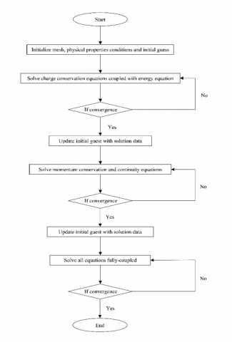
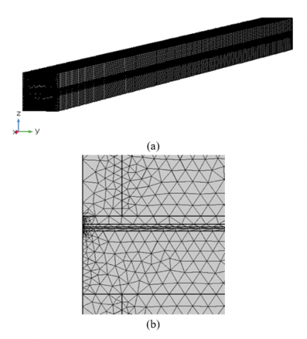
A three-dimensional FEM-based method CFD home-made code was used to solve the linear and non-linear governing equations developed in previous section. The detailed solution algorithm is depicted in Figure 2. A triangular mesh type was selected. In meshing process, first yz surface was meshed as shown in Figure 3 then it was swept along with x direction. The number of elements was changed for each case. However, the maximum total number of elements among all cases was 842356. To stabilize the numerical solution procedure, the mesh refinement was tuned so that finer meshes existed in active layers where more equations should be solved. The total solution time was in the range of 1 hr to 2 hr on a dual 3GHz Intel Xeon each with 64 GB memory.
Figure 2. Solution algorithm in simulation
Figure 3. (a) Mesh geometry, (b) Mesh distribution in active layers (yz view)
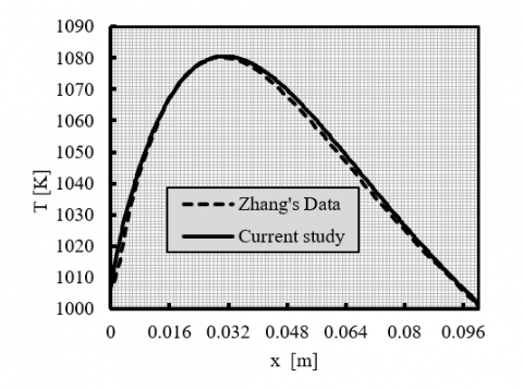
To prove the current model data precision, the solution output should be validated. For this aim, the current model outputs are compared to the data reported by Zhang et al. [28] and are shown in Figure 4. Note that all thermo-physical and geometrical data are kept the same as in the study of Zhang et al. [28]. The input data are listed in Table 2. The temperature distribution in the direction of fluid flow in the active anode layer is considered for validation task where all physics occur and are coupled. For this comparison, the R2 value indicating the deviation amount between two different studies is obtained by 0.99584 which is extremely close to one, showing that the current study has sufficient agreement with the data developed by Zhang et al. [28].
Figure 4. The comparison between current study and Zhang’s data [28]
Table 2. Thermo-physical parameters used in this study
|
Description |
Symbol |
Value |
|
Total pressure |
Ptot |
1 [atm] |
|
Operating temperature |
Tin |
1000 [K] |
|
Cell voltage |
Vcell |
0.7 [V] |
|
Hydrogen inlet mole fraction |
$x_{H_2, \text { in }}$ |
0.9 [1] |
|
Oxygen inlet mole fraction |
$x_{O_2, \text { in }}$ |
0.21 [1] |
|
Pressure loss at anode channel |
$\Delta P_a$ |
3000 [Pa] |
|
Pressure loss at cathode channel |
$\Delta P_c$ |
75 [Pa] |
|
Anode and cathode porosity |
$\varepsilon$ |
0.3 |
|
Cathode specific heat |
Cc |
430 [J/kg.K] |
|
Anode specific heat |
Ca |
450 [J/kg.K] |
|
Electrolyte specific heat |
Ce |
470 [J/kg.K] |
|
Cathode conductivity |
kc |
6 [W/m.K] |
|
Anode conductivity |
ka |
11 [W/m.K] |
|
Electrolyte conductivity |
ke |
2.7 [W/m.K] |
|
Cathode density |
$\rho_c$ |
3030 [m3/kg] |
|
Anode density |
$\rho_a$ |
3310 [m3/kg] |
|
Electrolyte density |
$\rho_e$ |
5160 [m3/kg] |
|
H2 dynamic viscosity |
$\mu_{H_2}$ |
6.162Í10-6+1.145 Í10-8T [Pa.s] |
|
H2O dynamic viscosity |
$\mu_{{H}_2 {O}}$ |
4.567Í10-6+2.209 Í10-8T [Pa.s] |
|
O2 dynamic viscosity |
$\mu_{O_2}$ |
1.668Í10-5+3.108 Í10-8T [Pa.s] |
|
N2 dynamic viscosity |
$\mu_{N_2}$q |
1.435Í10-5+2.642 Í10-8T [Pa.s] |
|
H2 conductivity |
$k_{H_2}$ |
0.08525+2.964 Í10-4T [W/m.K] |
|
H2O conductivity |
$k_{{H}_2 {O}}$ |
0.01430+9.782 Í10-5T [W/m.K] |
|
O2 conductivity |
$k_{O_2}$ |
0.01569+5.69 Í10-5T [W/m.K] |
|
N2 conductivity |
$k_{N_2}$ |
0.01258+5.444 Í10-5T [W/m.K] |
|
H2 specific heat |
$k_{N_2}$ |
13960 +0.95T [J/kg.K] |
|
H2O specific heat |
$C_{{H}_2 {O}}$ |
1639.2 +0.641T [J/kg.K] |
|
O2 specific heat |
$C_{O_2}$ |
876.80 +0.217T [J/kg.K] |
|
N2 specific heat |
$C_{{N}_2}$ |
935.6 +0.232T [J/kg.K] |
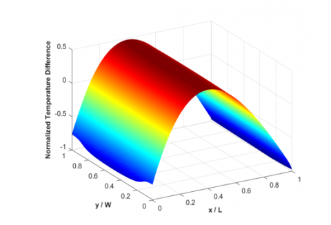
Figure 5 shows the normalized temperature difference (NTD) at the cell voltage of 0.7 V using geometrical parameters given in Table 1 within the anode-electrolyte intersection. The NTD value is defined as [11]:
$\nabla =\frac{T-{{T}_{average}}}{{{\left| T-{{T}_{average}} \right|}_{max}}}$ (22)
Figure 5. The normalized temperature difference (NTD) at the cell voltage of 0.7 V using geometrical parameters given in Table 1 within the anode-electrolyte intersection
As shown in Figure 5, the maximum NTD value occurs nearly at the middle of the cell but a little towards the cathode channel outlet. It is due to a large amount of pressure loss applied between inlet and outlet of cathode channel, leading to enlarge convection heat transfer coefficient at cathode channel and so the maximum point is moved towards the cathode channel outlet. The larger amount of pressure loss at cathode channel side compared to anode channel side is because of supplying sufficient oxygen at cathode active layer. It is also found out that the temperature distribution throughout the cell is not varied with y direction which is in agreement with Gong et al.’s study [11]. Therefore, the temperature variable is the function of x at a specified z and T-x plots can be considered for the aim of comparison of different cases.
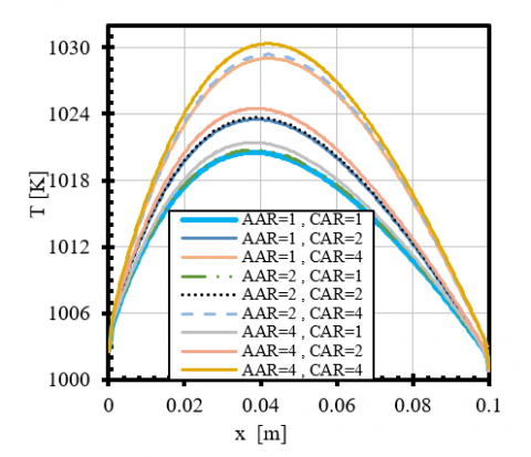
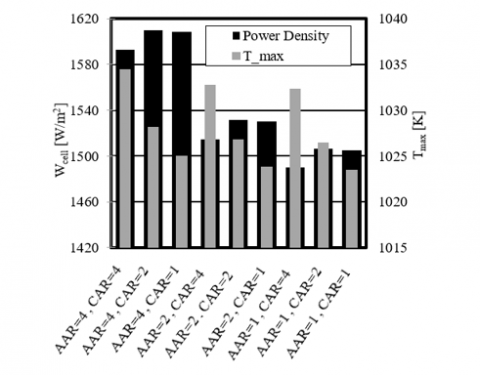
Figure 6 shows the effect of the rectangular cross section of electrode channels aspect ratio on the temperature profile along with flow direction based on a x-line crossing the center of the active anode at 0.7 V. AAR and CAR in this figure denote for the aspect ratio of anode and cathode rectangular cross sections, respectively. It is worth mentioning that to consider only geometrical effects of anode and cathode channels, the area of cross sections in all cases is constant as 1 mm2. As can be seen, the higher temperature is obtained with narrowing the cross section of channels so that the cell with channels of AAR = 4 and CAR = 4 reveals more temperature gradient and, in this case, the temperature changes from 1000 K to about 1030 K discovering a 30 K temperature difference while this value for the case of AAR = 1 and CAR = 1 is about 20 K, showing an about 33% decrease. However, narrowing at cathode channel side is obviously more effective in growing the temperature profile. However, Figure 7 discovers that varying the AAR value has more impact on the cell power density so that the maximum AAR value happens in narrow anode channel. Considering both maximum temperature and power density, the case with AAR = 4 and CAR = 1 reveals best performance while keeping the cell in lower temperature gradients.
Figure 6. Temperature profile along with flow direction in the middle of active anode for different aspect ratios of rectangular cross sections anode and cathode channels at cell voltage of 0.7 V
Figure 7. Maximum cell temperature and power density values for different anode and cathode channels aspect ratios at cell voltage of 0.7 V
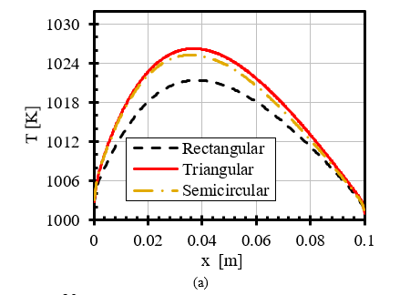
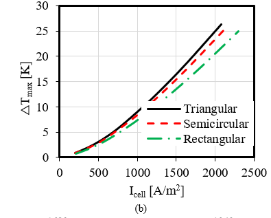
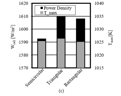
Figures 8(a)-(c) depict a comparison between different geometries including rectangular (with AAR = 4 and CAR = 1), triangular and semicircular in the cell performance and thermal behavior. As can be seen from Figure 8(a), a similar maximum temperature of 1025 K is achieved in these three geometries, however, the semicircular case produces the lowest power density of 1593 W/m2. The power density produced by the triangular and the rectangular cases are 1610 and 1608 W/m2, respectively, showing nearly the same value. The temperature profile along with the flow direction for three various geometries is presented in Figure 8(b). It is obvious that a similar temperature profile is observed for both triangular and rectangular geometries, touching the maximum point of 1026 K at location of x = 0.037 m. This value for the semicircular case is 1021 K, showing a 5 K decrease. Figure 8c presents the highest temperature difference in the cell with the current density of 200-2300 A/m2. The maximum temperature difference in both semicircular and triangular geometries is a little higher compared to the rectangular one which is the greatest amount, showing a 5.2% decrease.
Figure 8. Comparison of different geometries of channels effect: (a) the cell power density and maximum temperature, (b) temperature profile along with flow, (c) the cell maximum temperature difference
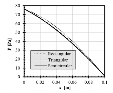
Figure 9 shows the pressure distribution in the middle of active anode at cell voltage of 0.7 V for different channel shapes. As can be seen, semicircular and triangular shapes show the same behaviour, however, rectangular shape shows a slight increase compared to the other two shapes.
Figure 9. The pressure distribution in the middle of active anode at cell voltage of 0.7 V for different channel shapes
4.1 Parametric study
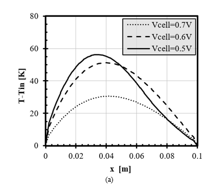
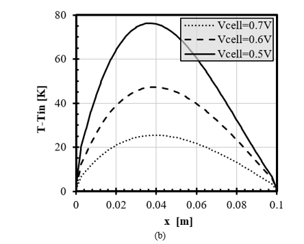
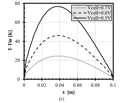
In this section, how the variations in the operating temperature, the inlet velocity and the cell voltage affect the temperature gradient inside the cell is investigated. Figure 10 depicts the cell voltage changes on temperature differences occurring in the middle of the anode active layer. As can be seen, the channels with rectangular shape show lower temperature gradient compared to the other two shapes. It is surprising that changing the voltage value from 0.6 to 0.5 V in the rectangular channel shape does not alter the temperature gradient profile significantly. However, this voltage change increases the maximum temperature difference from nearly 45 to 75 K in both triangular and semicircular shapes.
Figure 10. The cell voltage effect on the temperature changes for various channel shapes: (a) rectangular shape, (b) triangular shape, (c) semicircular shape
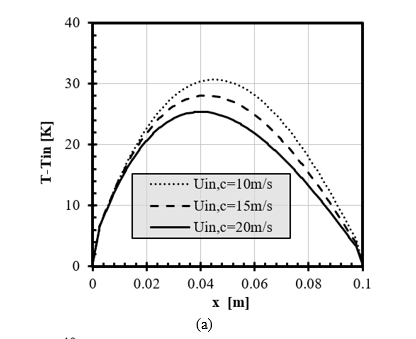
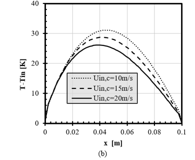
Figure 11. The inlet velocity effect on the temperature changes or various channel shapes: (a) rectangular shape, (b) triangular shape, (c) semicircular shape
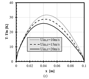
The inlet velocity effect on temperature difference occurring in the middle of the anode active layer is shown in Figure 11. To summarize the data presentation, as the velocity value in cathode channel is higher than this value in anode channel for reaching sufficient oxygen to the cathode functional layer, the cathode inlet velocity effect is examined. As shown, changing the inlet velocity discovers the same temperature gradient for all channel shapes. Furthermore, increasing the inlet velocity, decreases the temperature due to improving convection heat transfer in all cases. In fact, increasing the velocity value leads to transferring more heat produced within the cell.
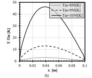
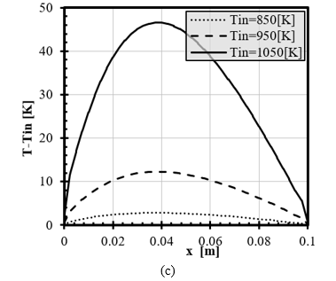
Figure 12. The operating temperature effect on the temperature changes for various channel shapes: (a) rectangular shape, (b) triangular shape, (c) semicircular shape
Finally, the operating temperature effect on temperature difference occurring in the middle of the anode active layer is shown in Figure 12. Results reveal that the rectangular shape presents more obstacles in the operating temperature changes considering the temperature gradient values compared to the two other shapes. The maximum temperature gradient for the rectangular shape is about 40 K in operating temperature of 1050 K, however, this value for both the triangular and the semicircular shapes is about 45 K.
A three-dimensional, FEM method based, is applied to be able to evaluate different shapes of anode and cathode channels cross sections in 1 mm 2 channels cross section area. Results show that narrowing the anode channel and widening the cathode channel in rectangular cross section cases increase the cell power density and decrease the temperature gradients which is more suitable in long-term operations. Finally, different geometries including rectangular, triangular and semicircular for the channels are examined to compare the cell performance and thermal gradient values. It is realized that by changing the channel geometries, almost the same thermal behavior is achieved. However, the semicircular case gives out less power density compared to the other two geometries and triangular geometry case produces the best performance. Thus, in the long-term applications of the planar SOFCs, the triangular and rectangular geometries for the anode and cathode channels are suggested. However, in the case of rectangular geometry, the aspect ratio should be tuned so that the narrower anode channel and wider cathode channel are preferred. Eventually, the parametric study revealed that the rectangular shape results in a lower temperature gradient in the variations of the cell voltage and the operating temperature situations compared to the triangular and the semicircular shapes. But, the inlet velocity values have the effect on the temperature gradient for all channel shapes.
|
A |
surface area per volume (m2.m-3) |
|
Cp |
isobaric specific heat (J.kg-1.K-1) |
|
d |
diffusional driving force (m-1) |
|
Dij |
multicomponent Fick’s diffusivity (m2.s-1) |
|
F |
Faraday’s constant (C.mol-1) |
|
F |
volume force (N.m-3) |
|
g |
gravity acceleration (m.s-2) |
|
I |
singular matrix (1) |
|
H |
Height (m) |
|
i |
volumetric charge source term (A.m-3) |
|
j |
mass flux vector (kg.m-2.s-1) |
|
k |
thermal conductivity (W.m-1.K-1) |
|
L |
cell length (m) |
|
M |
molecular weight (kg.mol-1) |
|
n |
number of electrons (1) |
|
p |
pressure (Pa) |
|
Q |
energy source term (W.m-3) |
|
Qm |
mass source term (kg.m-3.s-1) |
|
Ri |
ith mass source term (kg.m-3.s-1) |
|
Ru |
universal gas constant (J.mol-1.K-1) |
|
t |
thickness (m) |
|
T |
absolute temperature (K) |
|
u |
velocity vector (m.s-1) |
|
x |
mole fraction (1) |
|
W |
cell width (m) |
|
Greek symbols |
|
|
$\sigma$ |
conductivity (S. m-1) |
|
$\tau$ |
tortuosity of porous media (1) |
|
$\emptyset$ |
voltage (V) |
|
$\omega$ |
mass fraction (1) |
|
$\sigma$ |
conductivity (S.m-1) |
|
Subscripts |
|
|
a |
anode |
|
ac |
anode catalyst layer |
|
act |
activation |
|
av |
average |
|
c |
cathode |
|
cc |
cathode catalyst layer |
|
cell |
cell |
|
e |
electrolyte |
|
eff |
effective |
|
el |
electronic |
|
f |
fluid |
|
in |
inlet |
|
io |
ionic |
|
int |
interconnect |
|
j |
jth gaseous species |
|
max |
maximum |
|
OC |
open circuit |
|
s |
solid |
|
tot |
total |
[1] Singla, M.K., Nijhawan, P., Oberoi, A.S. (2021). Hydrogen fuel and fuel cell technology for cleaner future: A review. Environmental Science and Pollution Research, 28(13): 15607-15626. https://doi.org/10.1007/s11356-020-12231-8
[2] Chehrmonavari, H., Kakaee, A., Hosseini, S.E., Desideri, U., Tsatsaronis, G., Floerchinger, G., Paykani, A. (2023). Hybridizing solid oxide fuel cells with internal combustion engines for power and propulsion systems: A review. Renewable and Sustainable Energy Reviews, 171: 112982. https://doi.org/10.1016/j.rser.2022.112982
[3] Zhou, J., Alsharif, S., Alizadeh, A.A., Ali, M.A., Chaturvedi, R. (2024). Modeling and optimization of fuel cell systems combined with a gasifier for producing heat and electricity. International Journal of Hydrogen Energy, 52: 642-662. https://doi.org/10.1016/j.ijhydene .2023.01.132
[4] Singh, M., Zappa, D., Comini, E. (2021). Solid oxide fuel cell: Decade of progress, future perspectives and challenges. International Journal of Hydrogen Energy, 46(54): 27643-27674. https://doi.org/10.1016/j.ijhydene.2021.06.020
[5] Lee, Y.H., Ren, H., Wu, E.A., Fullerton, E.E., Meng, Y.S., Minh, N.Q. (2020). All-sputtered, superior power density thin-film solid oxide fuel cells with a novel nanofibrous ceramic cathode. Nano Letters, 20(5): 2943-2949. https://doi.org/10.1021/acs.nanolett.9b02344
[6] Ryu, S., Hwang, J., Jeong, W., Yu, W., Lee, S., Kim, K., Cha, S.W. (2023). A self-crystallized nanofibrous Ni-GDC anode by magnetron sputtering for low-temperature solid oxide fuel cells. ACS Applied Materials & Interfaces, 15(9): 11845-11852. http://doi.org/10.1021/acsami.2c22795
[7] Zhang, H.X., Yang, J.X., Wang, P.F., Yao, C.G., Yu, X.D., Shi, F.N. (2023). Novel cobalt-free perovskite PrBaFe1.9Mo0.1O5+δ as a cathode material for solid oxide fuel cells. Solid State Ionics, 391: 116144. http://doi.org/10.1016/j.ssi.2023.116144
[8] Xi, X., Huang, L., Chen, L., Liu, W., Liu, X., Luo, J.L., Fu, X.Z. (2023). Enhanced reaction kinetics of BCFZY-GDC-PrOx composite cathode for low-temperature solid oxide fuel cells. Electrochimica Acta, 439: 141617. https://doi.org/10.1016/j.electacta.2022.141617
[9] Rafaqat, M., Ali, G., Ahmad, N., Jafri, S.H.M., Atiq, S., Abbas, G., Raza, R. (2023). The substitution of La and Ba in X0.5Sr0.5Co0.8Mn0.2O3 as a perovskite cathode for low temperature solid oxide fuel cells. Journal of Alloys and Compounds, 937: 168214. https://doi.org/10.1016/j.jallcom.2022.168214
[10] Bai, J., Zhou, D., Zhu, X., Wang, N., Liang, Q., Chen, R., Yan, W. (2023). Bi0.5Sr0.5FeO3-δ perovskite B-site doped Ln (Nd, Sm) as cathode for high performance Co-free intermediate temperature solid oxide fuel cell. Ceramics International, 49(17): 28682-28692. https://doi.org/10.1016/j.ceramint.2023.06.124
[11] Gong, C., Tu, Z., Chan, S.H. (2023). A novel flow field design with flow re-distribution for advanced thermal management in Solid oxide fuel cell. Applied Energy, 331: 120364. https://doi.org/10.1016/j.apenergy.2022.120364
[12] Kim, J., Kim, D.H., Lee, W., Lee, S., Hong, J. (2021). A novel interconnect design for thermal management of a commercial-scale planar solid oxide fuel cell stack. Energy Conversion and Management, 246: 114682. https://doi.org/10.1016/j.enconman.2021.114682
[13] Quach, T.Q., Kim, Y.S., Lee, D.K., Ahn, K.Y., Lee, S., Bae, Y. (2023). Thermal management of Ammonia-fed Solid oxide fuel cells using a novel alternate flow interconnector. Energy Conversion and Management, 291: 117248. https://doi.org/10.1016/j.enconman.2023.117248
[14] Chellehbari, Y.M., Adavi, K., Amin, J.S., Zendehboudi, S. (2021). A numerical simulation to effectively assess impacts of flow channels characteristics on solid oxide fuel cell performance. Energy Conversion and Management, 244: 114280. https://doi.org/10.1016/j.enconman.2021.114280
[15] Kong, W., Han, Z., Lu, S., Gao, X., Wang, X. (2020). A novel interconnector design of SOFC. International Journal of Hydrogen Energy, 45(39): 20329-20338. https://doi.org/10.1016/j.ijhydene.2019.10.252
[16] Moreno-Blanco, J., Elizalde-Blancas, F., Riesco-Avila, J.M., Belman-Flores, J.M., Gallegos-Muñoz, A. (2019). On the effect of gas channels-electrode interface area on SOFCs performance. International Journal of Hydrogen Energy, 44(1): 446-456. https://doi.org/10.1016/j.ijhydene.2018.02.108
[17] Aghaei, A., Mahmoudimehr, J., Amanifard, N. (2024). The impact of gas flow channel design on dynamic performance of a solid oxide fuel cell. International Journal of Heat and Mass Transfer, 219: 124924. https://doi.org/10.1016/j.ijheatmasstransfer.2023.124924
[18] Wang, Y., Li, X., Guo, Z., Wang, K., Cao, Y. (2021). Effect of the reactant transportation on performance of a planar solid oxide fuel cell. Energies, 14(4): 1212. https://doi.org/ 10.3390/en14041212
[19] Fan, S., Zhu, P., Liu, Y., Yang, L., Jin, Z. (2022). Three-dimensional structure research of anode-supported planar solid oxide fuel cells. Journal of Energy Engineering, 148(3): 04022010. https://doi.org/10.1061/(ASCE)EY.1943-7897.0000837
[20] Lee, H.L., Han, N.G., Kim, M.S., Kim, Y.S., Kim, D.K. (2022). Studies on the effect of flow configuration on the temperature distribution and performance in a high current density region of solid oxide fuel cell. Applied Thermal Engineering, 206: 118120. https://doi.org/10.1016/j.applthermaleng.2022.118120
[21] Wang, C., Yang, J., Huang, W., Zhang, T., Yan, D., Pu, J., Li, J. (2018). Numerical simulation and analysis of thermal stress distributions for a planar solid oxide fuel cell stack with external manifold structure. International Journal of Hydrogen Energy, 43(45): 20900-20910. https://doi.org/10.1016/j.ijhydene.2018.08.076
[22] Xu, M., Li, T.S., Yang, M., Andersson, M., Fransson, I., Larsson, T., Sundén, B. (2016). Modeling of an anode supported solid oxide fuel cell focusing on thermal stresses. International Journal of Hydrogen Energy, 41(33): 14927-14940. https://doi.org/10.1016/j.ijhydene.2016.06.171
[23] Fang, X., Lin, Z. (2018). Numerical study on the mechanical stress and mechanical failure of planar solid oxide fuel cell. Applied Energy, 229: 63-68. https://doi.org/10.1016/j.apenergy.2018.07.077
[24] Li, G., Liao, Y., Cheng, J., Huo, H., Xu, J. (2024). Coupled electrochemical-thermo-stress analysis for methanol-fueled solid oxide fuel cells. Journal of The Electrochemical Society, 171(5): 054502. https://doi.org/10.1149/1945-7111/ad417d
[25] Zheng, J., Xiao, L., Wu, M., Lang, S., Zhang, Z., Chen, M., Yuan, J. (2022). Numerical analysis of thermal stress for a stack of planar solid oxide fuel cells. Energies, 15(1): 343. https://doi.org/10.3390/en15010343
[26] Jiang, C., Gu, Y., Guan, W., Ni, M., Sang, J., Zhong, Z., Singhal, S.C. (2020). Thermal stress analysis of solid oxide fuel cell with Z-type and serpentine-type channels considering pressure drop. Journal of the Electrochemical Society, 167(4): 044517. https://doi.org/10.1149/1945-7111/ab79aa
[27] Xia, W., Yang, Y., Wang, Q. (2009). Effects of operations and structural parameters on the one-cell stack performance of planar solid oxide fuel cell. Journal of Power Sources, 194(2): 886-898. https://doi.org/10.1016/j.jpowsour.2009.06.009
[28] Zhang, X., Wang, L., Espinoza, M., Li, T., Andersson, M. (2021). Numerical simulation of solid oxide fuel cells comparing different electrochemical kinetics. International Journal of Energy Research, 45(9): 12980-12995. https://doi.org/10.1002/er.6628
[29] Ghassemi, M., Kamvar, M., Steinberger-wilckens, R. (2020). Chapter 1-Introduction to fuel cells. Fundamentals of Heat and Fluid Flow in High Temperature Fuel Cells, 1-15. https://doi.org/10.1016/B978-0-12-815753-4.00001-4
[30] Hami, M., Mahmoudimehr, J. (2024). A comprehensive comparison of performances of anode-supported, cathode-supported, and electrolyte-supported solid oxide fuel cells during warming-up process. International Journal of Heat and Mass Transfer, 230: 125779. https://doi.org/10.1016/j.ijheatmasstransfer.2024.125779.
[31] Nield, D.A., Bejan, A. (2006). Convection in Porous Media. New York, NY: Springer New York. https://doi.org/10.1007/0-387-33431-9_6
[32] Batchelor, G.K. (2000). An Introduction to Fluid Dynamics. Cambridge University Press. http://doi.org/10.1017/CBO9780511800955
[33] Kamvar, M., Ghassemi, M., Steinberger-Wilckens, R. (2020). The numerical investigation of a planar single chamber solid oxide fuel cell performance with a focus on the support types. International Journal of Hydrogen Energy, 45(11): 7077-7087. https://doi.org/10.1016/j.ijhydene.2019. 12.220
[34] Taylor, R., Krishna, R. (1993). Multicomponent Mass Transfer. John Wiley & Sons.
[35] Kamvar, M. (2021). Comparative numerical study of co-and counter-flow configurations of an all-porous solid oxide fuel cell. Hydrogen, Fuel Cell & Energy Storage, 8(2): 77-93. https://doi.org/10.22104/ijhfc.2021.4712.1212
[36] Akhtar, N., Decent, S.P., Loghin, D., Kendall, K. (2009). A three-dimensional numerical model of a single-chamber solid oxide fuel cell. International Journal of Hydrogen Energy, 34(20): 8645-8663. https://doi.org/10.1016/j.ijhydene.2009.07.113
[37] Xu, H., Chen, B., Tan, P., Xuan, J., Maroto-Valer, M.M., Farrusseng, D., Ni, M. (2019). Modeling of all-porous solid oxide fuel cells with a focus on the electrolyte porosity design. Applied Energy, 235: 602-611. https://doi,org/10.1016/j.apenergy.2018.10.069
[38] Kamvar, M., Ghassemi, M., Rezaei, M. (2016). Effect of catalyst layer configuration on single chamber solid oxide fuel cell performance. Applied Thermal Engineering, 100: 98-104. https://doi.org/10.1016/j.applthermaleng.2016.01.128
[39] Andersson, M., Yuan, J., Sundén, B. (2013). SOFC modeling considering hydrogen and carbon monoxide as electrochemical reactants. Journal of Power Sources, 232: 42-54. https://doi.org/10.1016/j.jpowsour.2012.12.122
[40] Andersson, M., Yuan, J., Sundén, B. (2014). SOFC cell design optimization using the finite element method based CFD approach. Fuel Cells, 14(2): 177-188. https://doi.org/10.1002/fuce.201300160
[41] Alhazmi, N., Almutairi, G., Alenazey, F., AlOtaibi, B. (2021). Three-dimensional computational fluid dynamics modeling of button solid oxide fuel cell. Electrochimica Acta, 390: 138838. https://doi.org/10.1016/j.electacta.2021.138838
[42] Kamvar, M., Steinberger-Wilckens, R. (2021). Numerical investigation of a hydrogen-fuelled planar AP-SOFC performance with special focus on safe operation. Hydrogen, Fuel Cell & Energy Storage, 8(2): 113-125. https://doi.org/10.22104/ijhfc.2021.5181.1229