Manoj Kumar Panda![]() | Pruthiviraj Nemalipuri*
| Pruthiviraj Nemalipuri*![]() | Vivek Vitankar
| Vivek Vitankar![]() | Harish Chandra Das
| Harish Chandra Das![]() | Malay Kumar Pradhan
| Malay Kumar Pradhan![]()
© 2025 The authors. This article is published by IIETA and is licensed under the CC BY 4.0 license (http://creativecommons.org/licenses/by/4.0/).
OPEN ACCESS
To ensure robust simulations of technologically intricate industrial equipment such as furnaces and heaters, precise modelling of the computational domain is crucial, given the involvement of complex physics like combustion, turbulence, and radiation. Despite numerous numerical simulations conducted in this domain, there persists a significant disparity between simulation outcomes and existing experimental findings. This variance may stem from inadequate inclusion of appropriate combustion, radiation, turbulence models within the computational domain. In this study, we systematically examine the sensitivity of turbulence and radiation models. Various combustion simulation output parameters, such as flue gas temperature and velocity at different sections, as well as the mole fraction of reactant and product species are obtained by solving coupled partial differential equations governing combustion phenomena using two CFD software packages: ANSYS Fluent and Simcenter STAR CCM+. A non-premixed combustion model, paired with different radiation and turbulence models, is employed, and the methodology is validated by comparing the predicted results with the experimental data. Furthermore, this research delves into assessing the accuracy of simulated results from both CFD software packages. Results from both software packages closely align with experimental findings in the literature, particularly for the RNG k-ɛ turbulence model and the Discrete Ordinate (DO) radiation model. While Fluent offered marginally better agreement in the far-field oxygen distribution, STAR-CCM+ showed superior accuracy in predicting temperature, tangential velocity, and near-burner CO/CO₂ concentrations.
CFD, eddy-breakup, combustion, combustor
Combustors are very commonly employed in the process industry to generate heat by the combustion of fuel. The efficiency of the combustors is very critical for a favourable energy balance, productivity and profitability. If we consider gaseous fuel combustors, a wide variation in design is observed. Gaseous fuel is mixed with an excess oxidizer stream (mostly air) to get hot flue gases. These hot flue gases are then used to generate steam, pre-heat raw materials in the industry, etc. A typical design consists of a burner with separate channels for fuel and oxidizer, a mixing region, followed by a combustion zone. Burner plays a very critical role in mixing fuel and oxygen, resulting in the shape and size of the flame. The cylindrical mixing and combustion zone is sized such that the flame does not touch the walls and the heat transfer process is efficient [1]. Combustors are typically designed by following traditional design approaches, empirical correlations, experience and thumb rules [1]. Which often leads to over-design. The burner design is not flexible to burn different types of fuels and if not tuned properly, it leads to high NOx, CO, incomplete fuel combustion, red hot spots on the furnace walls and refractory failures. Due to high temperatures, it is not economical for designers to build experimental test rigs, which has led to engineering simulations for combustor design and analysis to gain wider acceptance [2-5]. The numerical simulations are an excellent tool not only for burner and furnace designers but also for the process industry, as they allow to validate the design, test new concepts and helps to arrive at best-operating conditions. It also facilitates solving the complex real-time problems of hot spot formations, refractory failures, tube leakages, NOx reduction, increasing combustion efficiency, etc.
While engineering simulations offer tremendous advantages, caution must be taken before implementing the results. CFD modelling involves solving the Navier Stokes equation, which is based on the law of conservation of mass and momentum [6-9]. However, many closures are required to account for turbulence, chemical reactions, combustion effects while using RANS approach for modelling random processes. Turbulence can be modelled using simpler and economical two-equation models (k-ɛ, k-ω etc.), full Reynold’s stress models, LES and most accurate but computationally expensive. To model the effect of radiation, several approaches like Discrete Ordinate, Grey and Surface to Surface radiation models are widely used. There are variations in combustion modelling approaches too. The simpler species transport modelling approach is commonly used but is computationally expensive to solve more species. As the combustion reactions are kinetically mixing controlled, the accuracy in modelling kinetic and mixing rates is very important. There are flamelet approaches to model the complex combustion process. On top of everything, the mesh has a significant effect on the solution. The point we would like to make is that the robustness of the model needs to be tested thoroughly before being used. Care should be taken to ensure that the CFD model of the combustor is validated, robust and is valid over different scales and operating conditions. The mesh type, size, shape and layout have a significant impact on the solution. All these model combinations should be analysed over different mesh sizes before applying it for innovation, design and debottlenecking.
Several experiments on natural gas combustors with constant velocity criteria have been conducted by Sayre et al. [10] at BERL. They have considered different scale combustors from 30 kW combustor to a full-scale industrial combustor of 12 MW, apart from evaluating the combustion performance near the burner zone and all combustion parameters in the combustor. These experimental data have been used by several authors [2, 3, 11-15] to validate CFD models. Capurso et al. [12] used the experimental data of BERL for the numerical simulation and compared their simulated results (temperature, velocity profiles and species concentration) with the experimental results for validation of the adopted CFD methodology. They blended the natural gas with 30% hydrogen and simulated the problem with different combustion and turbulence models. From the introduction of blended fuel in the combustor, they found that the production of CO is reduced to a great extent (57%). Yadav et al. [11] evaluated the effect of different radiation and RANS based turbulence models on the flow field of the natural gas combustor. From various simulations, they have concluded that the Discrete Ordinate radiation model predicted the flame temperature in agreement with the experimental results of BERL, but the peak velocity is over predicted. Yan et al. [13] simulated the natural gas combustor in reference to the BERL experimental data using two different radiation models, such as exponential wideband (EWB) model and weighted-sum-of-gray-gas (WSGG) model. From the simulated results, they commented that the EWB model performs better than WSGG model towards the prediction of combustion parameters. Dehaj et al. [16] extended the CFD simulation of BERL combustor towards the prediction NOx formation using Thermal NOx and Prompt NOx model for reducing the harmful impact on the environment. They calculated the formation of NOx using the mass fraction of NO, NO2 and N2O. From the simulations they found a suitable condition in improvement of safety and efficiency. Sharma and Prasad [2] predicted the burning rates and formation of NOx due to combustion in the natural gas combustor (BERL) using the non-premixed combustion model with Large Eddy Simulation turbulence model. They only mentioned about combustion process and did not discuss flow and thermal characteristics of the combustor. Puriya and Gupta [3] implemented numerical simulations on natural gas combustor using one combustion model with one turbulence model (Species transport model with RNG k-ɛ) and they observed that the results were considerably deviating with respect to the experimental data. Kuang et al. [17] performed the CFD simulations on natural gas combustor using the experimental data of BERL. They have validated their CFD methodology using different combustion and turbulence models, finally concluded that the Eddy-dissipation concept/ finite rate combustion model predicts well, but the deviation in the results is considerably high with respect to the experimental results. An experimental setup containing porous medium burner along with heat exchanger was developed for the heating of house by Dehaj et al. [16]. The effect on the thermal efficiency and production of NO has been observed by increasing the power and excess air ratio. From the experimentation, they have found that the NO concentration reduced with increase in the excess air and the maximum thermal efficiency was attained with excess air ratio of ½. The statistical optimization of burner for two gaseous and liquid-fired Combustors using alteration of the swirl number and quarl angle has been performed by Hajitaheri [14]. They have utilized OpenFOAM for the combustion analysis of BERL combustor. From the analysis, they concluded that at 23.20 quarl angle and 0.51 swirl number, the efficiency in fuel utilization improved. The outlet temperature profile of the combustor exhaust gases has been optimized [18] for utilizing the flue gas in the gas turbine. Motsamai has optimized the outlet temperature profile of the combustor exhaust gases by altering the throw angle of burner and inlet air swirl number.
From the above literature, it is clear that most of the efforts have been carried out on the species transport model using the Eddy dissipation model. In the literature, various authors have studied the effect of turbulence models and radiation models. However, most of their predictions deviate from the experimental data. The aspect of model robustness is not proven in existing literature. One point is clear that the species transport model using the eddy breakup combustion model didn’t predict the experimental data accurately. Although we have also used species transport approach with eddy dissipation model following the suggestions in the literature, the results were not in very good agreement. This might be due to high mathematical complexity of combustion problems, improper choice of various models available, and non-inclusion of the detailed chemical reaction of the combustion process. Hence there is a need to understand the accuracy and capabilities of combustion, radiation and turbulent models along with the appropriate coupling between them for better comparison.
In the present work, we have followed the non-premixed combustion modelling approach and used the chemical equilibrium (CE) model to resolve the flamelets, apart from studying the effect of different turbulence models and radiation models. This helps in developing a robust model with better predictive capability in simulating the furnaces used in industries. For industrial-scale furnaces, a major difficulty is the non-availability of temperatures, velocity and species data for validation. Hence, the approach of validation with the BERL experimental data will give us the confidence to model the industrial furnaces. In the current research, numerical simulations were performed on Natural gas combustor using ANSYS Fluent and STAR-CCM+, and the obtained output parameters are compared with the results of the experiments conducted at the Burner Engineering Research Laboratory (BERL), located at Sandia National Laboratory [10]. The present CFD analysis uses non-premixed probability density function (PDF) combustion model with different turbulence and radiation models such as standard k-ɛ model, realizable k- ɛ model, RNG k-ɛ model, standard k-$\omega$, SST k-$\omega$ turbulence model, Discrete Ordinate, P1 and Surface to Surface radiation models. From the series of simulation results obtained using ANSYS Fluent, it is observed that the Discrete Ordinate radiation model, RNG k-ɛ turbulence model coupled with the PDF combustion model predicts better results and are in close agreement with the experimental results. The same analysis is carried out using the above said best suitable turbulence and radiation models with PDF combustion model in STAR-CCM+ and the predicted results are found to be in good agreement with both, experimental and ANSYS Fluent results.
This work adds to the field of combustor CFD modeling in a number of novel ways. In order to show the consistency and limitations of two popular commercial solvers for simulating natural gas combustion in a swirl-stabilized BERL combustor, it first presents a thorough comparison of ANSYS Fluent and STAR-CCM+ using identical modeling frameworks. Second, using the non-premixed PDF combustion approach, the work systematically assesses three radiation models and five turbulence models, providing a clear comparison of their predictive accuracy with experimental data. The RNG k-ε turbulence model and the DO radiation model were found to be the most robust and reliable combination for capturing key combustor characteristics, such as temperature fields, axial and tangential velocity distributions, and species mole fractions (O₂, CO₂, and CO), with deviations within 8% of experiments.
This study also identifies solver-specific differences, demonstrating that although both solvers reproduce experimental trends well, STAR-CCM+ is more accurate in predicting near-burner CO and CO₂ distributions and tangential velocity, which are crucial for swirl-induced flame stabilization and the formation of product species. This work not only boosts confidence in RANS-based combustor simulations but also offers helpful advice for choosing model combinations to achieve high predictive fidelity in industrial combustion applications by developing a validated modeling framework across multiple turbulence-radiation combinations and two CFD platforms.
Natural gas combustors are mostly used in oil refineries. Natural gas and air are used as fuel and oxidizer in the natural gas combustor for the process of combustion.
2.1 Schematic diagram of the natural gas combustor
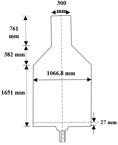
A 300 kW vertically fired natural gas combustor (BERL) is shown in Figure 1. It is the schematic drawing of the combustor with all dimensions.
Figure 1. Schematic diagram of the natural gas combustor
2.2 Boundary conditions
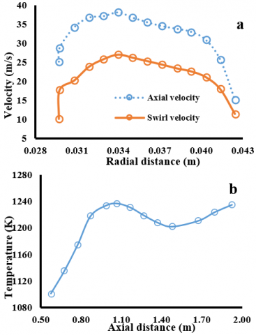
Natural gas enters the combustor radially through the 24 circumferential inlet ports at 22.7 kg/hr, 308 K. The composition of natural gas is given in Table 1. The swirling air comes through the annulus of the burner with a mean velocity of 31.25 m/s and 315 K. The swirl in the air is represented by the profile as shown in Figure 2(a).
Figure 2. (a) Axial and swirl velocity profiles, (b) Temperature profile
Table 1. Composition of natural gas
|
Species Molecular Formula |
Mass Fraction |
|
CH4 |
0.93312 |
|
N2 |
0.02195 |
|
C2H6 |
0.03081 |
|
C3H8 |
0.00266 |
|
C4H10 |
0.0035 |
|
CO2 |
0.00796 |
Table 2. Wall thermal boundary conditions
|
Wall Boundary |
Temperature (K) |
Emissivity |
|
Near inlet ducts |
312 |
0.5 |
|
Bluff body of front wall |
1173 |
0.5 |
|
Inlet duct |
1173 |
0.5 |
|
Quarl |
1273 |
0.5 |
|
Furnace bottom |
1100 |
0.5 |
|
Furnace cylinder |
Profile |
0.5 |
|
Furnace top |
1305 |
0.5 |
|
Chimney |
1370 |
0.5 |
The walls of the furnace were cooled by cooling tubes. Hence, there is a heat loss from the walls. The measured temperature on different walls is tabulated in Table 2 and Figure 2(b) shows the temperature profile on the cylinder wall due to the cooling tubes.
2.3 Mathematical modelling
Computational Fluid Dynamic analysis involves the solution of momentum balance equations along with the continuity equation. As the flow in the furnaces is highly turbulent, the turbulence models are used to model the turbulent stress terms. Among all the turbulence models, two equations turbulence models are preferred for the numerical simulations by considering the computational cost and accuracy [19, 20].
Continuity:
$\frac{\partial \rho}{\partial t}+\frac{\partial}{\partial x_i}\left(\rho u_i\right)=0$ (1)
Momentum equation:
$\frac{\partial}{\partial t}\left(\rho u_i\right)+\frac{\partial}{\partial x_i}\left(\rho u_i u_j\right)=-\frac{\partial P}{\partial x_i}+\frac{\partial}{\partial x_j}\left(\tau_{i j}-\rho u_i^{\prime} u_{i j}^{\prime}\right)+F_i$ (2)
where, $\tau_{i j}$= viscus stress tensor and $F_i$ is the body force.
$\tau_{i j}=\left[\mu\left(\frac{\partial u_i}{\partial x_j}+\frac{\partial u_j}{\partial x_i}-\frac{2}{3} \delta_{i j} \frac{\partial u_k}{\partial x_k}\right)\right]$ (3)
Turbulent kinetic energy:
$\frac{\partial(\rho k)}{\partial t}+\frac{\partial}{\partial x_i}\left(\rho u_i k\right)=\frac{\partial}{\partial x_i}\left(\frac{\mu_t}{\sigma_h} \frac{\partial k}{\partial x_i}\right)+P-\rho \varepsilon+\dot{\rho} k$ (4)
whereas turbulent kinetic energy production rate P is:
$P=\mu_t\left(\frac{\partial u_i}{\partial x_j}+\frac{\partial u_j}{\partial x_i}\right) \frac{\partial u_i}{\partial x_j}-\frac{2}{3} \frac{\partial u_i}{\partial x_i}\left(\rho k+\mu_t \frac{\partial u_i}{\partial x_i}\right)$ (5)
Energy Equation: The energy balance equation in the form of enthalpy is solved in the domain. The source term in the energy equation accounts for the heat generated due to combustion reactions [18].
$\frac{\partial(\rho h)}{\partial t}+\frac{\partial}{\partial x_i}\left(\rho u_i h\right)=\frac{\partial}{\partial x_i}\left(\Gamma_h \frac{\partial h}{\partial x_i}\right)+s_h$ (6)
where, $\Gamma_h=\left(\frac{\mu}{\sigma}+\frac{\mu_t}{\sigma_h}\right), \sigma_h$= turbulent Prandtl number.
Radiation Modelling: Radiation is an important mechanism of heat transfer. There are several approaches to model radiative heat transfer. One such approach is the Discrete Ordinate radiation model, which describes the radiative heat transfer in participating media and has been used in the present work. It simulates thermal radiation exchange between diffuse/specular surfaces forming a closed set [19].
Discrete Ordinate radiation model equation:
$\nabla \cdot\left(W_\lambda((\vec{p}, \vec{q})) \vec{q}\right)+\left(a_\lambda+\sigma_s\right)\left(W_\lambda((\vec{p}, \vec{q})) q\right)=a_\lambda n^2 W_{b \lambda} \frac{\sigma_s}{4 \pi}\left(W_\lambda((\vec{p}, \vec{q}))\right) \Phi \cdot\left(\vec{q}, \vec{q^{\prime}}\right) d \Omega^{\prime}$ (7)
2.3.1 Turbulence chemistry interaction
In the BERL combustor, natural gas is used as a fuel, which has methane as a significant fuel species. A simplified one-step reaction for methane combustion can be written as:
${CH}_4+2 {O}_2 \rightarrow {CO}_2+2 {H}_2 {O} \quad {DH}=-{Kcal} / {kg}$
This reaction is considered to be instantaneous and is highly exothermic.
The reaction rate can be written as:
$R_a=k C a^m$
When the average reaction rate is affected by the turbulence as well as the chemistry, this phenomenon is called turbulence-chemistry interactions. Different models are used to account for these turbulence-chemistry interaction effects.
2.3.2 Species transport approach
Species transport models account for this effect through turbulent diffusion between cells. Species transport model solves the mass fraction for each of the species in the domain [18]. This model becomes computationally expensive as transport equations for all the species are solved. Furthermore, the non-linearity in the rate expressions makes the solution stiffer.
Species transport equation:
$\frac{\partial}{\partial t}\left(\rho X_k\right)+\frac{\partial}{\partial X_j}\left(\rho u_i X_k\right)=\frac{\partial}{\partial X_i}\left(\rho D_k \frac{\partial X_k}{\partial x_i}\right)+\dot{z}_k$ (8)
The value of rate constant “K” is typically given in terms of Arrhenius equation.
$K=k_o e^{(-E / R T)}$
However, for instantaneous and very fast reactions, mixing is the rate-limiting step. Therefore, the eddy dissipation model is typically used. This model assumes that the fuel and the oxidant burn immediately when mixed. Hence, the reaction rate is governed by mixing intensity and turbulence.
2.3.3 Flamelet models
The term flamelet is used to describe a basic 0D or 1D laminar flame geometry. In flamelet models, the turbulence-chemistry interaction effects are handled through assumed shape probability density functions (PDFs) for the flamelet variables, which consider the impact of local species and temperature distributions [10, 19]. In addition, flame propagation models can be used to precisely model the movement of a flame front as a function of turbulence and chemical state. In flamelet models, a limited set of flamelet variables is used to represent the reacting flow system and define the thermochemical state within each CFD cell. Instead of solving the conservation equations for all species, the conservation equations are solved for the limited number of flamelet variables. The flamelet approach has reduced computational cost compared to the reacting species transport approach because a reduced number of transport equations are solved and the chemistry in the reaction mechanism is solved before the CFD simulation. The flamelet modelling approach is suitable for reacting flow systems in which the reaction timescale is shorter than the mixing timescale. This approach is useful for steady-burning furnaces and burners with full-load conditions in combustors. When flamelets are calculated, the detailed thermo-chemistry of the temperature and species within the flame is parameterized by two or more variables. The CE model assumes that the turbulent flow is in chemical equilibrium. Hence, chemistry is very fast compared to flow and mixing. This corresponds to the zero strain of the Steady Laminar Flamelet (SLF) model or the burnt state of the Flamelet Generated Manifold (FGM) model. The thermo-chemical state is parameterized by mixture fraction (Z) and enthalpy.
The mixture fraction Z is calculated using:
$Z=\frac{m_f}{m_f+m_{0 x}}$ (9)
The mixture fraction, denoted as Z, represents the local mass fraction of elements originating from the fuel stream relative to the total mass from both fuel and oxidizer streams. Specifically, mf is the total mass of all elements derived from the fuel stream at a given spatial location, while mox is the corresponding mass from the oxidizer stream. The mixture fraction Z is transported within the flow field through both convection and diffusion mechanisms. To capture the effects of turbulence on the mixing process, a presumed probability density function (PDF) is applied, which is defined as a function of the mean mixture fraction $\bar{Z}$ and its variance Zvar. This approach allows for the statistical treatment of turbulent fluctuations in Z. The variance Zvar itself can either be obtained by solving a dedicated transport equation or by using a simplified algebraic approximation.
2.3.4 Mixture fraction variance
The equation that is derived for the mixture fraction variance is:
$\frac{\partial}{\partial t}\left(\rho Z_{v a r}\right)+\nabla \cdot\left(\rho v Z_{v a r}-\frac{\mu_t}{S c_g} \nabla Z_{v a r}\right)=\frac{2 \mu_t}{S c_g}(\nabla Z)^2-c_d \rho \frac{\varepsilon}{k} Z_{v a r}$ (10)
where, the mixture fraction variance $Z_{ {var }}$ of each scaled mixture fraction [18] is calculated as: $Z_{ {var }}=\overline{(Z-\bar{Z})^2}$. $S c_g$ is the turbulent Schmidt number for the mixture fraction variance and $c_d$ is a scalar dissipation constant. To reduce the time of computing reaction outcomes during a simulation, lookup tables are generated before starting the simulation. These lookup tables provide reaction products and mixture properties for a chosen range of states. Table entries are generated for the instantaneous chemical conditions. In reality, turbulence effects are continually at work within the fluid system at timescales smaller than the simulation time-step.
A probability density function is assumed for the dependent quantities for accounting the turbulence effects and then sampled when integrating these quantities across the entire simulation time-step. The general form of the integration step is represented as:
$\widetilde{Q}=\int_0^1 Q(Z) P(Z) d Z$ (11)
When using the CE model, flamelets are solved at different enthalpy levels and cell temperatures are obtained by interpolating the flamelet table directly at the enthalpy that is being solved.
When the transport data is imported along with the chemical and thermodynamic data for flamelet generation, the molecular transport properties for Dynamic Viscosity, Molecular Diffusivity, and Thermal Conductivity are tabulated. Based on the properties of each species, kinetic theory is used to calculate the dynamic viscosity and thermal conductivity of each species. The molecular diffusivity is calculated from the unity Lewis number assumption. Mass fraction weighted averaging is then used to calculate the mixture diffusivity, while Mathur-Saxena averaging is used to calculate the mixture viscosity and thermal conductivity. The CE model assumes that what is mixed has reacted and reached chemical equilibrium. The model assumes that all species diffuse at the same rate, which is reasonable for turbulent flows with much higher turbulent diffusivity than molecular diffusivity. In addition to tracking the mixture fraction and its variance, when the CE model is active, additional heat loss ratio equations are solved.
2.3.5 Heat loss ratio
Heat gain or loss in the system indicates a deviation from ideal adiabatic conditions. To account for such non-adiabatic effects within the CFD domain, the flamelet table is extended by introducing a parameter called the heat loss ratio. This ratio quantifies the impact of thermal losses by representing the normalized difference in enthalpy between the actual cell enthalpy and the corresponding adiabatic enthalpy at the same mixture fraction [19]. Essentially, it captures how much energy has been lost (or gained) relative to an adiabatic flamelet, as a function of the local mixture fraction, allowing the model to more accurately reflect real combustion behaviour where heat transfer to walls, radiation, or other losses occur.
$\gamma=\frac{h_{a d}-h}{h_{a d}}$ (12)
where, $h_{a d}$ is the adiabatic enthalpy, h is the cell enthalpy and $h_{a d}$ is the sensible (or thermal) enthalpy.
The sensible enthalpy, $h_{a d}$, that is defined as:
$h_{ {sens }}=\Sigma_{k=0}^{N_s} Y_k\left(\int_{T_{\text {ref }}}^T C_{p, k} d T\right)$ (13)
$h_{a d}=(1-Z) h_{ {oxid }}+(Z) h_{ {fuel }}$ (14)
Temperature is stored in the table and then retrieved based on the table dimensions.
2.3.6 Tabulation for chemical equilibrium
The independent variables are: Mixture Fraction Z, Mixture Fraction Variance $Z_{ {var }}$ and Heat Loss Ratio (when using the Non-Adiabatic model) γ.
When the boundary condition values are given for Z and the streams are specified for Z = 1 (fuel stream) and Z = 0 (oxidizer stream), the value of any conserved scalar $\phi$ (concentration for a specific element) is calculated at any spatial location according to:
$\boldsymbol{\phi}=\boldsymbol{Z} \boldsymbol{{\phi}_f}+(\mathbf{1}-\boldsymbol{Z}) \boldsymbol{{\phi}_{o x}}$ (15)
where, $\phi_f$ and $\phi_{o x}$ represent the values of the conserved scalars in the fuel and oxidizer streams, respectively. Therefore, when Z is known, the concentration of any given element is also known at that location. When the elemental concentrations are known, Simcenter STAR-CCM+ passes them along with the initial temperature to an equilibrium routine which yields (a) the mass fractions of all species (b) the density (c) the temperature at that point (using a Gibbs free-energy minimization technique).
In a turbulent flow field, the mean value of any scalar quantity is obtained by integrating its instantaneous value over the joint probability density function (PDF) of the mixture fraction Z and enthalpy h:
$\bar{\phi}(\dot{Z}, \bar{h})=\int \phi(Z, h) P(Z, h) d Z\,\, d h$ (16)
A statistical independence assumption for $P(Z, h)$ can be made so that:
P(Z,h) = P(Z)P(h) (17)
The mean value of enthalpy is used in the calculation of:
$\bar{\phi}(\dot{Z}, \bar{h})=\int \phi(Z, \bar{h}) P(Z, h) \mathrm{d} Z$ (18)
The integrals in Eqs. (17) and (18) are pre-computed. When the value of an integral is needed during the calculation, a simple interpolation is all that is needed to provide the correct value.
β-PDF equation:
$\bar{P}(\xi)=\frac{\xi^{\alpha-1}(1-\xi)^{\beta-1} \Gamma(\alpha+\beta)}{\Gamma(\alpha) \Gamma(\beta)}$ (19)
where, $\Gamma(z)$ denotes the gamma function and the shape of the β-pdf depends on the values of parameters $\alpha$ and $\beta$. The parameters $\alpha$ and $\beta$ can be calculated from the mean and variance of mixture fraction $(\xi)$ at every location.
$\boldsymbol{\alpha}=\tilde{\xi}\left[\frac{\xi(1-\xi)}{\tilde{\xi}^{\prime \prime^2}}-1\right]$ (20)
$\boldsymbol{\beta}=(\mathbf{1}-\tilde{\boldsymbol{\xi}}) \frac{\alpha}{\tilde{\boldsymbol{\xi}}}$ (21)
where, $\tilde{\boldsymbol{\xi}}$ is the Favre mean of $\boldsymbol{\xi}$ and $\tilde{\boldsymbol{\xi}}^{\prime \prime 2}$ is the Favre-averaged variance of $\boldsymbol{\xi}$.
In the current approach, two-dimensional numerical simulations were performed on natural gas combustor (BERL) using non-premixed combustion PDF model described in the above section 2.2.2. The two-equation k-ɛ model was used for turbulence modelling and the DO radiation model for radiative heat transfer.
3.1 Discretization
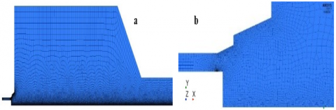
The 2D domain was discretized into small hexahedral volume elements as shown in Figure 3. Since the number of cells and node connectivity in the computation domain profoundly affects the solution as well as computational cost, meshing plays a decisive role in getting an accurate solution from the simulations. While executing mesh, one should be aware of creating a good mesh to capture the physics precisely in the region of importance so that the computational simulation results will be in close agreement with the real solution. The mesh quality can be assessed in terms of average quality, skewness and aspect ratio.
Figure 3. Meshed geometry of BERL combustor (a) 2D mesh, (b) Burner throat
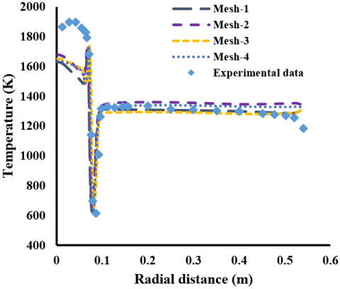
The numerical solution is dependent mainly on the discretization of the domain. So, for robust solutions, the simulations are performed for different types of mesh as described in Table 3. From several simulations using 4 different discretized domains, it is observed from Figure 4 that the solution remains independent of the number of elements and nodes for mesh-1. A very fine mesh is created in the burner quarl as mixing and combustion gets initiated. The velocity, thermal and density gradients are very high in this region. The resolution of this region is important as the flame shape and size are governed by the burner region.
3.2 Setup and solution
The non-premixed combustion model is selected for combustion modelling and state-relation is given as chemical equilibrium with inlet diffusion, followed by the generation of the PDF table. The combustion analysis is mostly dependent on the combustion model and the turbulent model used, as there is an interconnection between them. The turbulence viscosity calculated by the turbulent models is added to the molecular viscosity to get effective viscosity. This effective viscosity is used to calculate shear stress terms in Navier-Stokes equation. Thus, the choice of the turbulence model has a direct effect on flow and enthalpy predictions. Hence, in this work, we have studied the effect of two-equation turbulence models like standard k-ε model, realizable k-ɛ model, RNG k-ɛ model, standard k-ω model and SST k-ω model. The difference in these turbulence models is the mathematical formulation to calculate the eddy viscosity. As the temperatures in the furnaces are in the range of 1000-1800 K, radiative heat transfer becomes essential. There are several radiation models available like Discrete Ordinate, surface to surface radiation model and P1 model. The details of radiation models and their implementations are available more elaborately in the theory and user guides of Simcenter STAR-CCM+ and ANSYS Fluent.
Table 3. Different types of mesh for grid-independent solution
|
|
Number of Nodes |
No. of Elements |
Average Quality |
Average Skewness |
Average Aspect Ratio |
|
Mesh-1 |
37256 |
35958 |
0.9156 |
0.1056 |
1.1537 |
|
Mesh-2 |
60481 |
58698 |
0.9279 |
0.1686 |
1.1759 |
|
Mesh-3 |
81142 |
79351 |
0.9320 |
0.1261 |
1.1586 |
|
Mesh-4 |
117499 |
115159 |
0.9526 |
0.1425 |
1.1624 |
Figure 4. Grid independent test
The experienced CFD community is very well aware that for complex problems like combustion, CFD modelling is still the art. The right combination of the turbulence model and radiation model has an impact on the solution. Hence, to better understand the sensitivity of these models and develop a robust model, we have performed simulations by varying turbulence models and radiation models. In all the cases, the mesh and the non-premixed CE model were maintained the same.
In all the simulations, the Coupled algorithm is used for pressure-velocity coupling and the pressure equation was solved by PRESTO algorithm in ANSYS Fluent and SIMPLE algorithm in STAR CCM+. The remaining equations are solved by the second-order upwind scheme of Finite Volume Method (FVM) and the convergence criteria is used as 10e-6. Simcenter STAR-CCM+ and ANSYS Fluent are two commonly used software. In this work, we thought it is desirable to compare the predictions of both the software with same settings. That would also give the readers additional insight.
4.1 ANSYS Fluent
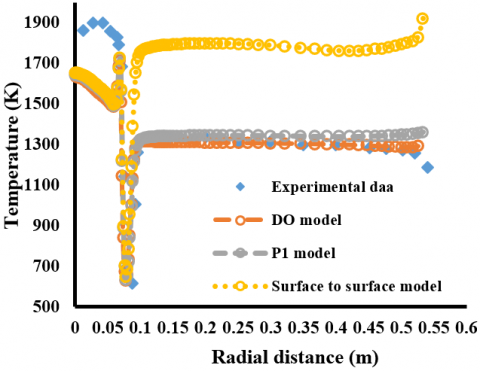
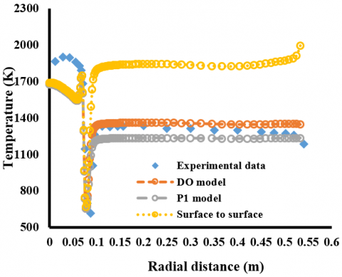
The k-ε turbulence model served as a baseline for solving the model discussed in section 2.3, and various radiation models were used to examine the impact of radiation. Figure 5 compares the temperature predictions in a natural gas combustor at 27 mm downstream of the burner throat. According to the findings, the Surface-to-Surface (S2S) model considerably overpredicts the flame temperature, whereas the Discrete Ordinates (DO) and P1 models exhibit good agreement with experimental measurements. This disparity results from the S2S model's assumption of only surface radiation exchange, which ignores the participating medium effects of combustion gases (H2O, CO2). However, volumetric radiation from the hot gas dominates in combustors; as a result, S2S is unable to accurately depict the actual heat transfer mechanism, producing unnaturally high predicted temperatures. In contrast, radiative transfer in a participating medium is explicitly taken into account in the P1 and DO models. The DO model offers a more detailed angular resolution, which enables it to capture the strong anisotropy of flame radiation and the impact of shadowing from geometrical features. This explains its superior performance compared to the P1 model, which approximates radiation as a diffusion process and performs fairly well for optically thick media.
Figure 5. Comparison of temperature at 27 mm downstream to the burner throat by experimental data with different radiation models using standard k-ɛ model
Additional simulations were conducted using various turbulence models, including standard k-ω, RNG k-ε, realizable k-ε, and SST k-ω, in order to better understand the role of turbulence modeling. The results, presented in Figures 5-10, demonstrate that turbulence models strongly influence the prediction of temperature distribution, flame stabilization, and mixing behaviour. In general, swirling flows and recirculation zones which are essential for flame anchoring and mixing enhancement in combustor operation are better captured by the realizable and RNG k-ε models. In particular, the RNG k-ε model improves accuracy in highly strained and swirling flame regions by taking into account small-scale turbulence and strain rate effects. Predictions for flows with strong streamline curvature, like those around the burner quarl or swirling jets, are improved by the realizable k-ε model. On the other hand, the k-ω family of models (standard and SST) tends to resolve near-wall regions better, which can improve flame wall interaction predictions, but may underperform in capturing large-scale recirculation compared to k-ε variants. The SST model, being a blend of k-ε and k-ω, offers improved robustness, yet in strongly swirling combustor flows, the RNG k-ε often remains the most reliable due to its ability to handle jet breakdown and recirculation dynamics more effectively.
It is observed that among all the radiation models, the Discrete Ordinates (DO) model provides the most reliable results across all turbulence models when coupled with the non-premixed combustion model. This can be attributed to the fact that the DO model solves the radiative transfer equation along a finite number of discrete solid angles, thereby accounting for the anisotropic nature of flame radiation and the volumetric absorption/emission from combustion products such as CO₂, H₂O, and soot. In contrast, simplified models either approximate radiation as isotropic diffusion (P1) or neglect gas-phase participation altogether (S2S), which leads to discrepancies in predicted flame temperature and, consequently, combustion chemistry. Since radiation directly influences the local flame temperature, it also governs the reaction rates, equilibrium composition, and formation of intermediate species, making DO the most physically consistent choice in capturing coupled turbulence–radiation–chemistry interactions.
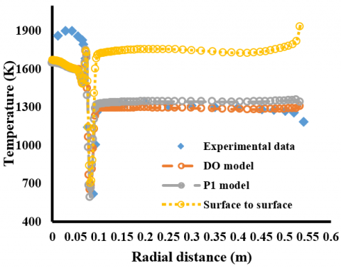
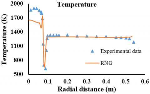
Figure 6. Comparison of temperature at 27 mm downstream to the burner throat by experimental data with different radiation models using RNG k-ɛ model
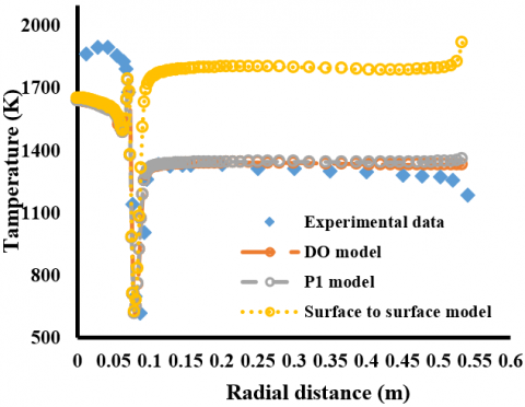
Figure 7. Comparison of temperature at 27 mm downstream to the burner throat by experimental data with different radiation models using realizable k-ɛ model
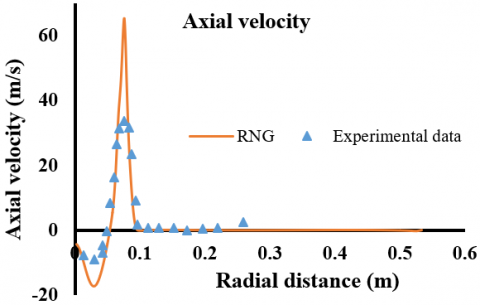
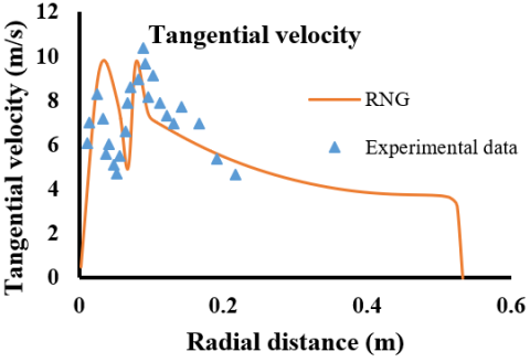
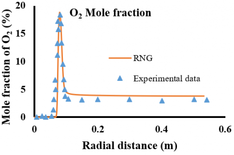
Figure 10(a)-(d) displays the predictions of additional important flow and combustion parameters for the RNG k-ε turbulence model, including axial velocity, tangential velocity, and oxygen mole fraction. Effective jet penetration from the burner throat and the development of recirculation zones downstream both essential for flame stabilization are highlighted by the axial velocity field. Because it accounts for strain-rate effects and offers better accuracy for swirling, recirculating flows than the standard k-ε model, the RNG k-ε model successfully captures these features. The swirler's function in giving the flow angular momentum and creating a central recirculation zone is illustrated by the tangential velocity distribution. This recirculation zone improves flame stability by encouraging fuel and oxidizer mixing. The RNG k-ε model is particularly suited here, as its formulation includes swirl modification terms that allow for better representation of vortex breakdown and swirl-induced turbulence. In the same manner, the profiles of the oxygen mole fraction reveal information about the mixing and consumption of fuel and oxidizer. Because of the intense combustion and quick mixing, steep oxygen gradients are seen in the vicinity of the burner. Because it more accurately depicts turbulent mixing in shear layers and the entrainment of ambient air into the flame zone, the RNG k-ε model is able to predict these gradients. This results in a realistic simulation of oxidation rates and species depletion when combined with the DO model, which guarantees precise local temperature prediction. Therefore, the best option for natural gas combustor simulations is the combination of the RNG k-ε turbulence model and DO radiation model, which not only accurately predicts temperature profiles but also consistently represents flow dynamics and species transport.
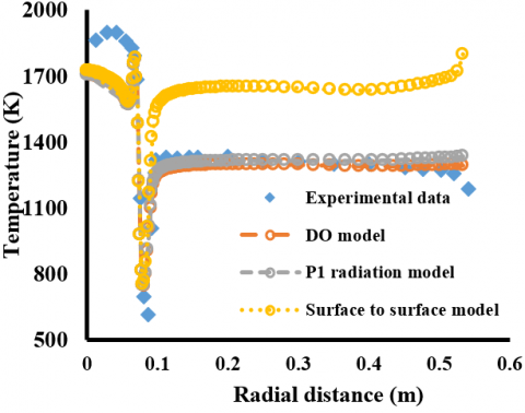
Figure 8. Comparison of temperature at 27 mm downstream of the burner throat by experimental data with different radiation models using the standard k-ω model
Figure 9. Comparison of temperature at 27 mm downstream of the burner throat by experimental data with different radiation models using SST k-ω model
Therefore, it can be concluded that the most accurate predictions of important parameters like temperature, axial velocity, tangential velocity, and oxygen mole fraction in the natural gas combustor are obtained from simulations that use the RNG k-ε turbulence model in conjunction with the Discrete Ordinates (DO) radiation model and the non-premixed PDF combustion model. Because each model has complementary strengths in capturing the underlying physics, this combination performs best. By adding strain-rate corrections and swirl modifications, the RNG k-ε model enhances the standard k-ε model and is especially useful for simulating the highly swirling, recirculating flows found in combustors. Accurately predicting these recirculation zones guarantees a realistic flow field, which is essential for flame stabilization and improved fuel and oxidizer mixing.
Figure 10. Comparison of temperature, Axial velocity, tangential velocity and O2 mole fraction at 27 mm downstream to the burner throat by experimental data using non-premixed combustion (PDF) model with RNG k-ɛ turbulence model and Discrete Ordinate radiation model on XY-plot
By solving the radiative transfer equation in several discrete directions, the DO radiation model improves accuracy even further and accounts for the anisotropic and volumetric nature of radiation from hot combustion gases (CO₂, H₂O). Predicting reaction rates, equilibrium composition, and pollutant formation requires precise radiative heat transfer modeling because radiation has a significant impact on the local flame temperature. This complexity is not captured by models such as P1 or S2S, which either ignore gas-phase radiation completely or oversimplify radiation as isotropic diffusion. The non-premixed PDF combustion model, on the other hand, statistically represents the fluctuations of scalar quantities like mixture fraction in order to account for turbulence–chemistry interactions. In contrast to turbulent mixing, this works especially well for natural gas combustion, where the flame is controlled by mixing and chemical kinetics take place on far shorter timescales. The PDF model guarantees that oxygen consumption, flame structure, and heat release are accurately represented by resolving local mixing effects and coupling them with turbulence and radiation. Together, these three models offer a framework that is both physically sound and self-consistent: the non-premixed PDF model captures the turbulence–chemistry coupling, DO guarantees proper energy transfer through radiation, and RNG k-ε precisely resolves the flow and mixing dynamics. This synergy explains why this modeling approach results in the most reliable predictions of velocity fields, temperature distribution, and species concentrations in the natural gas combustor.
4.2 STAR CCM+
Keeping the same model combinations from ANSYS Fluent simulations, i.e. the RNG k-ɛ turbulence model, DO radiation model and non-premixed PDF model, the simulations are done using Simcenter-STAR-CCM+ for the same discretized domain used in ANSYS Fluent.
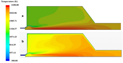
Figure 11. Comparison of temperature contours a) ANSYS Fluent, b) STAR-CCM+
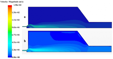
Figures 11 and 12 depict the temperature and velocity variation between ANSYS Fluent and STAR CCM+, respectively. They are shown on the same scale. The changes in colour intensity can be ignored as both the software have different colour schemes. The detailed comparative analysis of the output parameters (temperature, velocities, mole fractions of various species) using ANSYS Fluent and STAR-CCM+ is performed using the XY-Plot (Figures 13-18) at the distance of 27 mm from the burner throat, because the highly reacting zone is near the throat.
Figure 12. Comparison of velocity contours a) ANSYS Fluent, b) STAR-CCM+
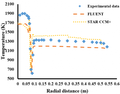
Figure 13. Comparison of temperature predictions at 27 mm from the burner throat between Fluent, STAR-CCM+ and experimental data
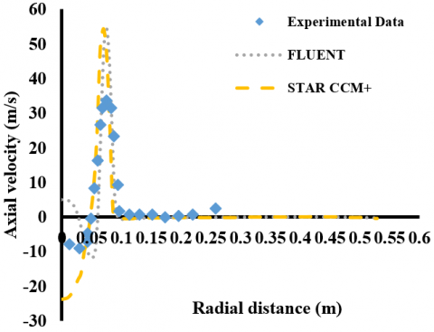
Figure 14. Comparison of axial velocity predictions at 27 mm from the burner throat between Fluent, STAR-CCM+ and experimental data
The close agreement between the STAR-CCM+ and ANSYS Fluent predictions is evident, suggesting that both solvers consistently capture the natural gas combustor's dominant flow and combustion characteristics. Both tools, however, underestimate the burner region's temperature. Usually, this systematic underprediction is ascribed to shortcomings in radiation treatment and modeling of the turbulence–chemistry interaction. Strong turbulence–chemistry coupling, localized extinction/re-ignition, steep scalar gradients, and highly mixing-controlled combustion are all present in the near-burner zone. Although the non-premixed PDF method employed in both solvers offers a statistical depiction of turbulence–chemistry interactions, it might not completely address scalar dissipation and sub-grid scale fluctuations in mixture fraction, which frequently results in an underestimation of the local flame temperature. Furthermore, if grid resolution or angular discretization are not sufficiently improved, radiation models even DO can smooth temperature fields, which results in somewhat colder predictions than experimental data.
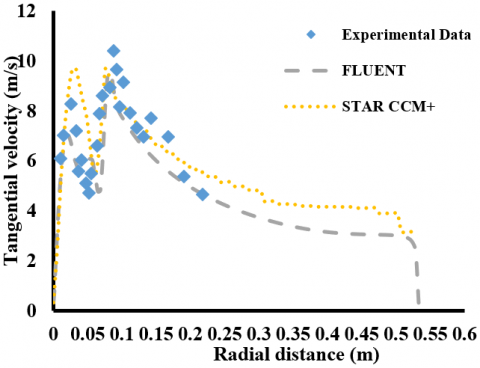
Figure 15. Comparison of tangential velocity predictions at 27 mm from the burner throat between Fluent, STAR-CCM+ and experimental data
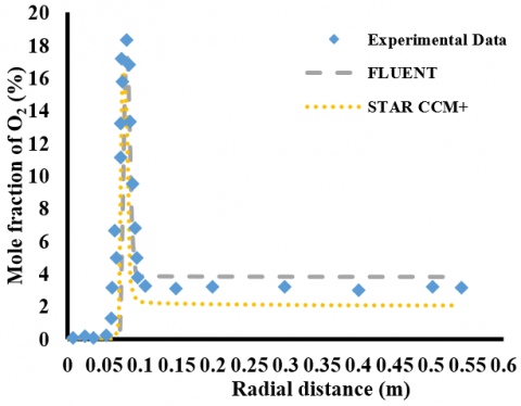
Figure 16. Comparison of O2 mole fraction predictions at 27 mm from the burner throat between Fluent, STAR-CCM+ and experimental data
From the axial velocity comparison, it is noted that STAR-CCM+ is able to capture the overall trend of jet penetration and recirculation in the burner region, though both solvers overpredict the peak velocity. This behavior arises due to the inherent sensitivity of turbulence models to jet breakup and shear layer growth. High swirl and strong velocity gradients near the burner throat tend to amplify turbulence anisotropy, which two-equation RANS models (such as RNG k-ε or realizable k-ε) approximate only in an isotropic sense. This often results in excess jet momentum prediction, producing a higher axial velocity peak than observed experimentally. Despite this, the correct trend reproduction by STAR-CCM+ indicates that the solver is effectively capturing the large-scale recirculation dynamics essential for flame stabilization.
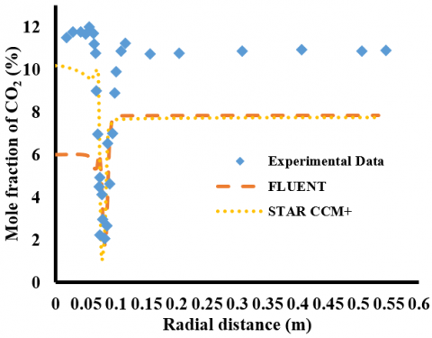
Figure 17. Comparison of CO2 mole fraction predictions at 27 mm from the burner throat between Fluent, STAR-CCM+ and experimental data
For the tangential velocity, the predictions from both solvers are comparable, but STAR-CCM+ demonstrates superior capability in reproducing the first velocity peak. This improved performance can be linked to differences in numerical schemes and discretization practices between STAR-CCM+ and Fluent. STAR-CCM+ employs a polyhedral meshing strategy that can more effectively resolve swirl-dominated flows with complex geometrical features, reducing numerical diffusion in angular momentum transport. Since tangential velocity directly controls swirl strength and the formation of the central recirculation zone, accurately predicting the first peak is critical to capturing the correct flame anchoring mechanism. The better agreement of STAR-CCM+ in this aspect suggests that its solver settings and discretization offer an advantage in handling swirl-induced secondary flows.
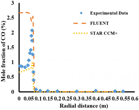
The mole fraction plots indicate that both STAR CCM+ and ANSYS Fluent provide broadly similar predictions, confirming that both solvers capture the dominant combustion chemistry and mixing processes in the natural gas combustor. However, notable differences emerge when examining specific regions of the flame. It can be seen that Fluent tends to overpredict mole fractions in regions away from the burner, while STAR-CCM+ slightly underpredicts them in the same zones. These differences can be attributed to variations in numerical schemes, discretization practices, and turbulence chemistry interaction modeling between the two solvers. In the far-field, where scalar gradients are weaker and mixing is more diffusion-dominated, solver specific numerical diffusion and grid resolution sensitivity can significantly affect predictions of minor species. Overprediction by Fluent suggests relatively stronger mixing or slower consumption rates predicted in the far field, while underprediction by STAR-CCM+ points toward more aggressive mixing and dilution of products with entrained air.
Figure 18. Comparison of CO mole fraction predictions at 27 mm from the burner throat between Fluent, STAR-CCM+ and experimental data
The CO₂ mole fraction plots provide additional insight into these discrepancies. Near the burner region, STAR-CCM+ predictions are in very close agreement with experimental data, indicating that the solver is effectively capturing the primary combustion zone, where rapid oxidation of hydrocarbons takes place. This accuracy highlights STAR CCM+’s ability to represent the near-burner mixing and flame stabilization process, where small errors in turbulence chemistry coupling can have a large impact on product species formation. On the other hand, both solvers underpredict CO₂ mole fraction in regions away from the burner. This underprediction suggests incomplete conversion of intermediate species or insufficient residence time in the post-flame zone within the models. Physically, this can be linked to limitations of the RANS-based non-premixed PDF combustion approach, which may not fully resolve slow-chemistry processes, minor species oxidation, or spatial intermittency in turbulent mixing. Furthermore, radiative heat losses in the post-flame region reduce local temperatures, slowing reaction rates. If radiation is not perfectly captured, this can also contribute to lower predicted CO₂ concentrations compared to experiments.
In Figure 18, CO is a sensitive marker of local equivalence ratio, temperature, and residence time. In the near-burner zone, fuel–rich pockets and strong scalar dissipation promote CO formation through incomplete oxidation of CH radicals and partial conversion of intermediate species. As the flow convects downstream and entrains more oxidizer, CO is oxidized to CO₂ provided temperature and radicals remain sufficiently high. The close agreement of STAR CCM+ with the experimental CO in the burner region indicates that its combination of RNG k-ε (capturing swirl-induced recirculation and shear-layer mixing), non-premixed PDF (representing fluctuations in mixture fraction and conditional chemistry), and DO radiation (setting the correct thermal field in a participating medium) is resolving the delicate balance between CO production in rich, high-strain layers and its subsequent burnout in slightly leaner, well-mixed zones.
Parity of model selections across solvers. With identical physical sub-models (RNG k-ε, non-premixed PDF, DO/WSGGM), the two codes should converge to the same physics. The remaining differences primarily reflect numerics: discretization schemes, flux limiters, pressure–velocity coupling, and mesh topology that control numerical diffusion of mixture fraction and enthalpy. Slightly different dissipation of scalar gradients changes peak CO by altering (i) the thickness of mixing layers, (ii) the local scalar dissipation rate χ, and (iii) the residence time in high-temperature zones—hence the small solver-to-solver offsets you see outside the burner core. Agreement across Figures 13-18 with Sayre et al. [10]. The collective comparison temperature, axial/tangential velocities, O₂, CO₂, and CO shows ANSYS Fluent and STAR-CCM+ are both in close agreement with the experiments of Sayre et al. [10], capturing the jet breakdown, the participating radiation field and the mixing-controlled chemistry.
The present investigation deals with the combustion analysis of the BERL combustor using two widely employed CFD solvers, ANSYS Fluent and STAR-CCM+, with a focus on assessing the influence of different turbulence and radiation modeling approaches. The simulations were carried out using the non-premixed PDF combustion model, which is particularly suitable for natural gas flames where the combustion process is predominantly controlled by turbulent mixing. To evaluate model sensitivity, the flame characteristics were tested across five turbulence models and three radiation models, analyzed independently to determine their predictive capability.
The RNG k-ε turbulence model in conjunction with the Discrete Ordinates (DO) radiation model consistently demonstrated the best agreement with experimental measurements among the combinations that were examined. The strengths of the RNG k-ε model in handling swirling, recirculating flows, and high-strain shear layer features that dominate combustor aerodynamics physically justify this result. By adding a strain-rate correction and taking into consideration how swirl affects turbulence dissipation, the RNG formulation enhances shear-layer mixing and the capture of the central recirculation zone, two crucial processes for flame stabilization. Similar to this, the DO radiation model accurately represents the anisotropic and volumetric radiation from combustion products by solving the radiative transfer equation along discrete angular directions. Since radiative heat loss directly governs flame temperature, which in turn controls reaction rates, the superior thermal predictions of the DO model translate into more realistic combustion chemistry outcomes.
Key combustion parameters like temperature fields, axial velocity, and tangential velocity profiles were accurately reproduced in the numerical results obtained through this combination. The models' ability to resolve the momentum exchange between the swirling jets and the recirculating core was demonstrated by the close agreement between the predicted flame temperatures and velocity fields from both solvers, Fluent and STAR CCM+, and the experimental data. Other turbulence-radiation combinations, on the other hand, displayed observable variations, either over- or under-predicting peak temperatures and velocities. These differences result from either oversimplified radiation models (e.g., P1 or Surface-to-Surface) that ignore directional dependence and participating medium effects, or from the intrinsic limitations of some turbulence models (e.g., standard k-ε or k-ω), which cannot adequately capture the anisotropy of swirling turbulence.
Overall, the comparison demonstrated that both CFD solvers produced results that were within 8% of the experimental values, demonstrating the modeling strategy's resilience. Crucially, the RNG k-ε and DO combination's consistent performance across both solvers illustrates that it offers a computationally effective and physically dependable framework for simulating real combustor performance. This demonstrates the importance of carefully choosing turbulence-radiation models for precise flame simulations and provides assurance regarding the predictive power of RANS-based CFD for real-world gas turbine combustor analysis.
Future studies can concentrate on expanding this framework to more complicated fuels, like liquid fuels, hydrogen-enriched blends, and syngas, where finite-rate kinetics and intricate turbulence–chemistry interactions are crucial. Predictions of unstable mixing and flame dynamics may be further enhanced by the use of high-fidelity turbulence techniques (LES or hybrid RANS–LES) and sophisticated combustion models (e.g., FGM, EDC). To improve thermal and emissions accuracy, non-gray radiation models, pollutant formation sub-models, and conjugate heat transfer (CHT) should also be included. Developing reliable and computationally efficient predictive tools will require efforts toward reduced-order modeling and validation under a broader range of operating conditions in order to support industrial deployment.
The authors extend their sincere gratitude to Dr. Meghana Thimmappa, Assistant Professor in the Department of HSS at ITER, SOA University, Bhubaneswar, for her invaluable assistance in refining the manuscript. Her meticulous editing and keen eye for detail significantly improved the English language and corrected any grammatical inconsistencies, ultimately enhancing the quality of the work.
|
$\boldsymbol{R_{i, r}}$ |
Chosen source term |
|
$\boldsymbol{\vec{p}}$ |
position vector |
|
S |
path length |
|
K |
absorption coefficient |
|
Φ |
scattering phase function |
|
G |
const.=4 |
|
Z |
Mixture Fraction |
|
$\boldsymbol{v}^{\prime}$ |
stoichiometric coefficient |
|
$\boldsymbol{Y_k}$ |
mass fraction of the Kth species |
|
T |
temperature |
|
$\boldsymbol{{h}_{a d}}$ |
adiabatic enthalpy |
|
$\overline{\boldsymbol{P}}(\boldsymbol{\xi})$ |
$\boldsymbol \beta$ probability function |
|
$\boldsymbol{\vec{q}}$ |
direction vector |
|
$\vec{\boldsymbol{q}^{\prime}}$ |
scattering direction vector |
|
$\boldsymbol{\sigma_s}$ |
scattering coefficient |
|
X |
mass fraction |
|
H |
const.=0.5 |
|
$\dot{\boldsymbol{Z}}_\boldsymbol k$ |
source term |
|
$\boldsymbol{T_{ {ref }}}$ |
reference temperature |
|
$\boldsymbol{C_{p, k}}$ |
specific heat of the kth species |
|
$\boldsymbol{\delta_{i j}}$ |
isotropic second order tensor |
|
$\boldsymbol{W_\lambda(\vec p, \vec{q})}$ |
Radiation intensity at wavelength $\boldsymbol \lambda$ |
|
DO |
Discrete Ordinate |
|
FVM |
Finite Volume Method |
[1] Baukal Jr., C.E. (2004). Industrial Burners Handbook. CRC Press.
[2] Sharma, S., Prasad, D.S. (2014). Modelling of non- premixed methane BERL combustor through CFD approaches and prediction of methane burning. International Journal of Latest Technology in Engineering, Management & Applied Science, 3(12): 68-71. https://www.ijltemas.in/DigitalLibrary/Vol.3Issue12/68-71.pdf.
[3] Puriya, A., Gupta, R. (2013). Simulation of non-premixed natural gas flame. International Journal of Science and Research, 2(5): 97-100. https://www.semanticscholar.org/paper/Simulation-of-Non-Premixed-Natural-Gas-Flame-Puriya-Gupta/3c6b5e33e62dd679951538cde638696f43d9b59c.
[4] Aminian, J., Shahhosseini, S., Bayat, M. (2010). Investigation of temperature and flow fields in an alternative design of industrial cracking furnaces using CFD. Iranian Journal of Chemical Engineering, 7(3): 61-73.
[5] Nemalipuri, P., Das, H.C., Pradhan, M.K. (2020). Simulation of emission from coal-fired power plant. In: Biswal, B., Sarkar, B., Mahanta, P. (eds) Advances in Mechanical Engineering. Lecture Notes in Mechanical Engineering. Springer, Singapore. https://doi.org/10.1007/978-981-15-0124-1_87
[6] Versteeg, H.K., Malalasekera, W. (1995). An Introduction to Computational Fluid Dynamics: The Finite Volume Method. John Wiley & Sons Inc., 605 Third Avenue, New York, NY 10158. https://gidropraktikum.narod.ru/Versteeg-Malalasekera.pdf.
[7] Nemalipuri, P., Pradhan, D.M.K. (2018). Prediction of air pollutants emitting from chimney of a CHP using CFD. International Journal of Scientific & Engineering Research, 9(4): 105-110.
[8] Nemalipuri, P., Singh, V., Das, H.C., Pradhan, M.K., Vitankar, V. (2024). Consequence analysis of heptane multiple pool fire in a dike. Proceedings of the Institution of Mechanical Engineers, Part C: Journal of Mechanical Engineering Science, 238(5): 1811-1827. https://doi.org/10.1177/09544062231181813
[9] Nemalipuri, P., Singh, V., Vitankar, V., Das, H.C., Pradhan, M.K. (2024). Numerical prediction of fire dynamics and the safety zone in large-scale multiple pool fire in a dike using flamelet model. The Canadian Journal of Chemical Engineering, 102(1): 11-29. https://doi.org/10.1002/cjce.25094
[10] Sayre, A., Lallemant, N., Dugue, J., Weber, R. (1993). Scaling characteristics of the aerodynamics and low NOx properties of industrial natural gas burners scaling 400 study. Part 4. 300 kW BERL test results. Topical Report, National Technical Reports Library - NTIS.
[11] Yadav, S. (2018). Simplified numerical simulation of BERL combustor and prediction of NOx formation. In Proceedings of the 7th International and 45th National Conference on Fluid Mechanics and Fluid Power (FMFP): IIT Bombay, Mumbai, India. https://www.researchgate.net/publication/331134987_Simplified_Numerical_Simulation_of_BERL_Combustor_and_Prediction_of_NOx_Formation.
[12] Capurso, T., Ceglie, V., Fornarelli, F., Torresi, M., Camporeale, S.M. (2020). CFD analysis of the combustion in the BERL burner fueled with a hydrogen-natural gas mixture. E3S Web of Conferences, 197: 10002. https://doi.org/10.1051/e3sconf/202019710002
[13] Yan, L., Yue, G., He, B. (2016). Application of an efficient exponential wide band model for the natural gas combustion simulation in a 300 kW BERL burner furnace. Applied Thermal Engineering, 94: 209-220. https://doi.org/10.1016/j.applthermaleng.2015.09.109
[14] Hajitaheri, S. (2012). Design optimization and combustion simulation of two gaseous and liquid-fired combustors. Doctoral dissertation, University of Waterloo.
[15] Magnussen, B.F., Hjertager, B.H. (1977). On mathematical modeling of turbulent combustion with special emphasis on soot formation and combustion. Symposium (International) on Combustion, 16(1): 719-729. https://doi.org/10.1016/S0082-0784(77)80366-4
[16] Dehaj, M.S., Ebrahimi, R., Shams, M., Farzaneh, M. (2017). Experimental analysis of natural gas combustion in a porous burner. Experimental Thermal and Fluid Science, 84: 134-143. https://doi.org/10.1016/j.expthermflusci.2017.01.023
[17] Kuang, C., Hu, L., Zhang, X., Lin, Y., Kostiuk, L.W. (2019). An experimental study on the burning rates of n-heptane pool fires with various lip heights in cross flow. Combustion and Flame, 201: 93-103. https://doi.org/10.1016/j.combustflame.2018.12.011
[18] Motsamai, O.S. (2009). Optimisation techniques for combustor design. Doctoral dissertation, University of Pretoria.
[19] Ahmad, T., Plee, S.L., Myers, J.P. (2024). Fluent Theory Guide. p. 814. https://ansyshelp.ansys.com/public/account/secured?returnurl=/Views/Secured/corp/v242/en/flu_th/flu_th.html.
[20] Nemalipuri, P., Singh, V., Vitankar, V., Das, H.C., Pradhan, M.K., Jena, S. (2024). Predicting the safety zone and fire dynamics of heptane multiple pool fire in a square dike using flamelet-generated manifold model. Journal of the Brazilian Society of Mechanical Sciences and Engineering, 47(1): 44. https://doi.org/10.1007/s40430-024-05363-2