Collective Slip Results on Mhd Unstable Flow on Porous Stretching Sheet

An incompressible two-dimensional MHD electronically controlling fluid flow across a porous stretched surface is studied in the context of thermal emission. As shown in Figure 1, the horizontal and vertical directions are represented by the x- and y-axes, respectively, in a two-dimensional coordinate system. A thin sheet that is positioned and completely aligned with the x-axis is metaphorically compared to a metal plate, as shown. Along the x-axis, the sheet is moving continuously in the positive x-direction at a variable speed while meeting the criteria $\lambda t<1$ for a positive constant and stretching rate. The magnetic field, the magnetic field, denoted by the letter "x", is a coordinate that changes with distance from the origin over the surface. The magnetic field energy is denoted by B₀. It is anticipated that the induced magnetic field will be significantly smaller than the applied magnetic field since it is constrained by the charge's velocity. The equations that explain the flow are as follows:

$\left(\frac{\partial u}{\partial x}\right)+\left(\frac{\partial v}{\partial y}\right)=0$                 (1)

$\begin{gathered}\frac{\partial u}{\partial t}+u\left(\frac{\partial u}{\partial x}\right)+v\left(\frac{\partial u}{\partial y}\right)=v\left(1+\frac{1}{\beta}\right) \frac{\partial^2 u}{\partial y^2}-\frac{\sigma B(x)^2 u}{\rho}  -\left(T_{\infty}-T\right) g \beta_T-\left(C_{\infty}-C\right) g \beta_C-\frac{v u}{k_1}\end{gathered}$,             (2)

$\begin{aligned} & \frac{\partial \mathrm{T}}{\partial \mathrm{t}}+\mathrm{u}\left(\frac{\partial \mathrm{T}}{\partial \mathrm{x}}\right)+v\left(\frac{\partial \mathrm{T}}{\partial \mathrm{y}}\right)  =\alpha\left(1+\frac{16 \mathrm{~T}_{\infty}^3 \sigma^*}{3 \mathrm{k}^* \kappa}\right) \frac{\partial^2 \mathrm{~T}}{\partial \mathrm{y}^2}+\mathrm{Du} \frac{\partial^2 \mathrm{C}}{\partial \mathrm{y}^2},\end{aligned}$                  (3)

$\frac{\partial \mathrm{C}}{\partial \mathrm{t}}+\mathrm{u}\left(\frac{\partial \mathrm{x}}{\partial \mathrm{C}}\right)^{-1}+v\left(\frac{\partial \mathrm{y}}{\partial \mathrm{C}}\right)^{-1}=\mathrm{D}_{\mathrm{M}} \frac{\partial^2 \mathrm{C}}{\partial \mathrm{y}^2}$.           (4)

1.png

Figure 1. Configuration and coordinate system

The preceding description provides an overview of the model's boundary conditions.

$\begin{gathered}\mathrm{u}=\mathrm{U}(\mathrm{x}, \mathrm{t})+\mathrm{U}_{\mathrm{s}}, \mathrm{T}=\mathrm{T}_{\infty}+\mathrm{T}_0\left(\frac{\mathrm{ax}}{2 v(1-\lambda \mathrm{t})^2}\right)+\mathrm{T}_{\mathrm{s}}, \\ C=C_{\infty}+C_0\left(\frac{2 v(1-\lambda t)^2}{a x}\right)^{-1}+C_{s,},\text{at} \, \mathrm{y}=0\end{gathered}$                (5)

$u \rightarrow 0, T-T_{\infty} \rightarrow 0, C-C_{\infty} \rightarrow 0,$

as $y \rightarrow \infty$

as such $0 \leq T_0 \leq T_w$ and $0 \leq C_0 \leq C_w$ are applicable if $(1-\lambda t)>0$. Eq. (1) is fulfilled by defining the stream functions $\mathrm{u}=\left(\frac{\partial \psi}{\partial x}\right), v=\left(\frac{\partial \psi}{\partial y}\right)$.

Let's introduce the following dimensionless functions:

$\begin{gathered}\eta=\sqrt{\frac{a}{v(1-\lambda t)}} y, \quad \psi=\sqrt{\left(\frac{(1-\lambda t)}{a v}\right)^{-1}} x f(\eta) \\ C=C_{\infty}+C_0\left(\frac{a x}{2 v(1-\lambda t)^2}\right) \phi(\eta) . \\ T=T+T_0\left(\frac{a x}{2 v(1-\lambda t)^2}\right) \theta(\eta),\end{gathered}$                       (6)

Replacing Eq. (6) into (2), (3) and (4) we get the following.

$\begin{gathered}\left(1+\frac{1}{\beta}\right) \\ f^{\prime \prime \prime}(\eta)+f(\eta) f^{\prime \prime}(\eta)-f^{\prime}(\eta)^2-\delta\left(\frac{\eta}{2} f^{\prime \prime}(\eta)+f^{\prime}(\eta)\right) \\ -\left(M^2+k\right) f(\eta)+\frac{G r}{2} \theta(\eta)+\frac{G c}{2} f(\eta)=0,\end{gathered}$                    (7)

$\begin{gathered}\frac{1+\mathrm{R}}{\operatorname{Pr}} \theta^{\prime \prime}(\eta)+\operatorname{Duf}^{\prime \prime}(\eta)+\mathrm{f}(\eta) \theta^{\prime}(\eta)-\mathrm{f}^{\prime}(\eta) \theta(\eta) \\ -\frac{\lambda}{2 \mathrm{a}} \eta \theta^{\prime}(\eta)-\frac{2 \lambda}{\mathrm{a}} \theta(\eta)=0,\end{gathered}$                    (8)

$\begin{aligned} & \phi^{\prime \prime}(\eta)+\operatorname{Sc}\left(\phi(\eta) \phi^{\prime}(\eta)-\phi^{\prime}(\eta) \phi(\eta)\right) \\ & -\operatorname{Sc} \delta\left(2 \phi(\eta)+\frac{\eta}{2} \phi^{\prime}(\eta)\right)=0 .\end{aligned}$                             (9)

The transmuted extremity positions regarding the phenomena are:

$\begin{aligned} & \mathrm{f}_{\mathrm{W}}=\mathrm{f}(0), \frac{\mathrm{f}^{\prime}(0)-1}{\mathrm{~s}_{\mathrm{f}}}=\mathrm{f}^{\prime \prime}(0), \frac{\theta(0)-1}{\mathrm{~s}_\theta}=\theta^{\prime}(0)  , \frac{\phi(0)-1}{\mathrm{~s}_{\mathrm{f}}}=\phi^{\prime}(0) \\ & f^{\prime}(\eta) \rightarrow 0, \theta(\eta) \rightarrow 0, \phi(\eta) \rightarrow 0 \text { as } \eta \rightarrow \infty,\end{aligned}$                        (10)

where,

$\begin{aligned}& \delta=\frac{\lambda}{a}, \mathrm{Gr}=\frac{\mathrm{g} \beta_T T_0}{\mathrm{a} v}, \mathrm{Gc}=\frac{\mathrm{g} \beta_C C_0}{\mathrm{a} v}, \operatorname{Pr}=\frac{v}{\alpha}, \mathrm{R}=\frac{16 \mathrm{~T}^3{ }_{\infty} \sigma^*}{3 \mathrm{k}^* \kappa}, \\& \mathrm{M}=\sqrt{\frac{\sigma}{\rho \mathrm{a}}} B_0, \mathrm{Sc}=\frac{v}{D_M}, \mathrm{Du}=\frac{D_M C_0}{v \mathrm{~T}_0} . \\&\end{aligned}$

The local skin resistance coefficient S_f, local Nusselt number Nu, and local Sherwood number Sh are among the engineering-relevant physical characteristics, and they are described as:

$S_f=\frac{\mu}{\rho U_w^2}\left(\frac{\partial u}{\partial y}\right)_{y=0}$               (11)

$\mathrm{Nu}=\frac{\mathrm{x}}{\kappa\left(\mathrm{T}_{\mathrm{w}}-\mathrm{T}_{\mathrm{y}}\right)}\left[\kappa\left(\frac{\partial \mathrm{T}}{\partial \mathrm{y}}\right)_{\mathrm{y}=0}-\frac{4 \sigma^*}{3 \mathrm{k}^*}\left(\frac{\partial \mathrm{T}^4}{\partial \mathrm{y}}\right)_{\mathrm{y}=0}\right]$,                      (12)

$S h=-\frac{x}{\left(C_w-C_{\infty}\right)}\left(\frac{\partial C}{\partial y}\right)_{y=0}$                    (13)

By substituting Eq. (6) into (11) to (13) we can obtain the dimensionless form of equations

$\mathrm{S}_{\mathrm{fr}}=\sqrt{\operatorname{Re}_{\mathrm{X}} \mathrm{S}_{\mathrm{f}}}, \mathrm{Nu}_{\mathrm{r}}=\frac{\mathrm{Nu}}{\sqrt{\operatorname{Re}_{\mathrm{X}}}}=-[1+\mathrm{R}] \theta^{\prime}(0), \mathrm{Sh}_{\mathrm{r}}=\frac{\mathrm{Sh}}{\sqrt{\operatorname{Re}_{\mathrm{X}}}}=-\mathrm{f}^{\prime}(0)$,

Here, $R e_x$ is the local Reynolds number, defined as $\frac{U_w x}{v} \mathrm{Sh}_r$, $N u_r$ and $S f_r$ symbolizes the decreased Sherwood number, the decreased Nusselt number, and the decreased skin friction.

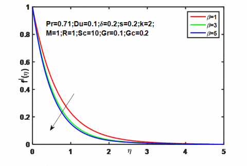
In order to enhance comprehension of the issue, Figures 2(a) and (b) with and without slip present graphical representations of the impacts of many factors on temperature, velocity, and concentration. As viscosity increases, flow momentum decreases, raising the Casson variable β and subsequently lowering the flow's velocity. This is seen in Figures 2(a) and 2(b).

1.png

(a) Control of Casson variable on displacement Rate without slip

2.png

(b). Control of Casson variable on displacement Rate with slip

Figures 2. Control of Casson variable on displacement rate

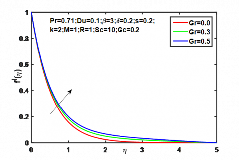
The differences in velocity profiles for various thermal Gasthof number values, Gr, are shown in Figures 3(a) and 3(b). It may be described as the thermal buoyant force divided by the viscous hydrodynamic force. Impact of this force is fruitful to a greater extent in the alliance of free convection, which rises momentum rate of the flow.

3a.png

(a) Displacement rate with respect to solutal Grashof number on velocity profiles without slip

3b.png

(b) Displacement rate with respect to solutal Grashof number on velocity distributions with slip

Figure 3. Displacement rate with respect to solutal Grashof number

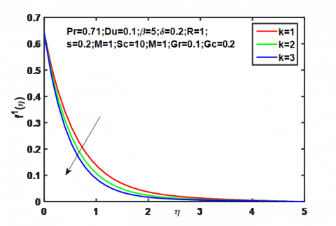
The portrayal of displacement rate has been represented in Figures 4(a) and 4(b). As porosity (k) increases while keeping other parameters constant, the velocity and density at the borderline also increase. The permeable medium becomes less favorable, resulting in a decrease in flow velocity.

4a.png

(a) Porosity's effect on non-slip velocity profiles

4b.png

(b) Porosity's effect on velocity profiles with slip

Figure 4. Porosity's effect on non-slip velocity profiles

5a.png

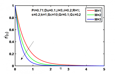
(a) Magnetic parameter control on slippage-free displacement profiles

5b.png

(b) Controlling the magnetic parameter on displacement patterns that involve slip

Figure 5. Magnetic parameter control on displacement profiles

By interacting with the magnetic field, the generated currents produce the immune force, an opposing force that lowers velocity. The acceleration of the flow decreases as the magnetic variable increases, as shown in Figures 5(a) and 5(b).

The effects of the radiation variable are shown in Figures 6(a) and 6(b). The displacement rate of the flow increases as the heat emission parameter increases. This is because the density of the thermal boundary layer increases with an increased radiation parameter.

6a.png

(a) Impact of the heat emission parameter on velocity profiles in the absence of slip

6b.png

(b) Consequence of heat emission parameter on velocity distributions with slip

Figure 6. Consequence of heat emission parameter on velocity distributions

Figures 7(a) and 7(b) show that, when suction is increased, the fluid flow velocity decreases due to decreased diffusion and a thinner fluid layer at the surface. The Prandtl number, or the ratio of fluid flow ease to heat conduction ease, is responsible for much of this occurrence.

Figures 8(a) and 8(b) demonstrate how the flow temperature rises as the heat emission parameter increases. The increase in heat emission parameter is attributed to the growth in thermal boundary layer density.

7a.png

(a) Performance of different suction parameter levels without any slippage

7b.png

(b) Speed profile for different suction parameter values with slip

Figure 7. Performance of different suction parameter levels on velocity profiles

8a.png

(a) Temperature profiles in the presence of slip, specifically examining the emission parameter

8b.png

(b) Temperature profiles in the presence of slip, specifically examining the emission parameter

Figure 8. Differences in temperature profiles for various heat emission parameter values

9a.png

(a) Temperature profiles in the absence of slip, specifically examining the Prandtl number

9b.png

(b) Temperature profiles in the presence of slip, specifically examining the Prandtl number

Figure 9. Temperature profiles specifically under the influence of Prandtl number

10a.png

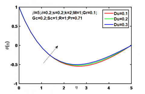
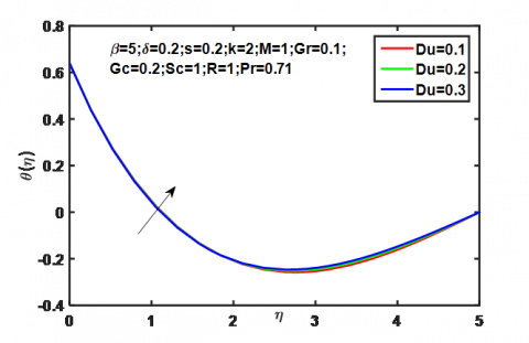
(a) Result of Dufour variable on thermal profiles with slip

10b.png

(b) Result of Dufour variable on thermal profiles with slip

Figure 10. Result of Dufour variable on thermal profiles

Heat conductivity and Prandtl number have an inverse relationship, as seen in Figures 9(a) and 9(b). This relationship is observed as a decrease in the boundary layer temperature as the Prandtl number grows.

As the Dufour number rises, so does the fluid's temperature. This is seen in Figures 10(a) and 10(b).

Figures 11(a) and 11(b) show how the Schmidt number affects concentration profiles. The mixture diffusivity reduces with increasing Schmidt number, facilitating a more even distribution of the solutal effect. Consequently, the concentration drops more gradually.

11a.png

(a) Results of concentration with reference to Schmidt number without slip

11b.png

(b) Results of concentration with reference to Schmidt number with slip

Figure 11. Results of concentration with reference to Schmidt number

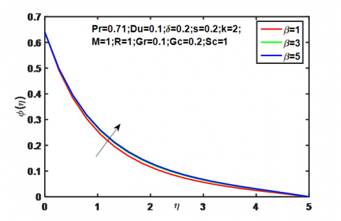
A fluid with a high viscosity and an increase in congregation is produced by increasing the Casson parameter. Figures 12(a) and 12(b) depict this.

12a.png

(a) Impression of Casson parameter on concentration profiles without slip

12b.png

(b) Impression of Casson parameter on concentration profiles with slip

Figure 12. Impression of Casson parameter on concentration profiles

A comparison analysis was conducted for the friction coefficient $-f^{\prime \prime}(0)$ at the surface and the rate of heat transfer -θ'(0) in order to verify the present findings and evaluate the accuracy of the continuing analysis.

Table 1 shows that increasing the stretching parameter increases the amount of skin friction.

Table 1. Comparing different values of $\delta$ when $f_w=\mathrm{M}=\mathrm{Gr}=\mathrm{Gc}=\mathrm{S}_f=0$

Table 2 illustrates how the skin friction coefficient varies in the absence of suction in accordance with the findings of [21], extending slip parameters as the magnetic variable M rises. We can observe that due to rise in magnetic parameter skin friction enlarges significantly owing to Lorentz forces generated by electromagnetic forces.

Table 2. Examination of $-f^{\prime \prime}(0)$ different values of M when f_w=δ=S_f=0

Table 3 displays a comparison between the present heat transfer rate numbers and those from [23]. It has been demonstrated that the Prandtl number has a significant impact on the heat transfer rate. As the Prandtl number rises, so does the rate of heat transport.

Table 3. Distinguishing of heat exchange rate -θ'(0) when $\mathrm{M}=\mathrm{f}_w=\mathrm{S}_f=\mathrm{S}_\theta=\delta=\mathrm{Gr}=\mathrm{Gc}=\mathrm{R}=0$