Rajesh Kumar Chandrawat* | Varun Joshi
© 2021 IIETA. This article is published by IIETA and is licensed under the CC BY 4.0 license (http://creativecommons.org/licenses/by/4.0/).
OPEN ACCESS
In this paper, the unsteady magnetohydrodynamic (MHD) Couette flow of two non-Newtonian immiscible fluids micropolar and micropolar dusty (fluid-particle suspension) are considered in the horizontal channel with heat transfer. A comprehensive mathematical model and computational simulation with the modified cubic B-Spline-Differential Quadrature method (MCB-DQM) is described for unsteady flow. The coupled partial differential equation for fluid and particle-phase are formulated and the effect of viscous dissipation, Joule heating, Hall current, and other hydrodynamic and solutal parameters i. e. Reynolds number, Eckert number, particle concentration parameter, Eringen micropolar material parameter, time, viscosity ratio, and density ratio on the flow rate, micro rotation, and temperature characteristics were investigated. The analysis of obtained results reveals that the fluids and particle velocities are slightly decreasing with Hartmann number, and increasing with time, ion-slip, and Hall parameters. Microrotation declined with Microrotations dropped significantly with ion-slip and Hall parameter and grown Hartman number. The temperature begins to rise as time, Hartman number, and Eckert number grow and declined with Ion-slip and Hall parameter.
micropolar fluid, immiscible fluid, unsteady flow, modified cubic b-spline, differential quadrature method
Hall current with ion slip has significant roles in various scientific processes including magnetohydrodynamic reactors, refrigeration coils, hall accelerators, flowmeters, and also in-flight magneto-aerodynamics. In the presence of a strong magnetic field, the effect of the Hall current and ion slip is important. As a result, it is essential to include the effect of the magnetohydrodynamics formulation, Hall current, and ion slip terms in the spectrum of functionalities such as a solid-state fuel-powered MHD engine. Inferred from these facts, many studies into MHD flows in the presence of Hall and ion slip currents have been conducted. The effect of ion slip on MHD energy monitoring of plasma flow around a blunt body is investigated by Yoshino et al. [1]. Elahi et al. [2] investigated the peristaltic flow of Jeffrey fluid in a non-uniform rectangular channel with Hall and ion slip effects and discussed the trapping phenomenon of MHD flow. Krishna and Chamkha [3] explored the Hall and Ion-slip implications for the MHD convective flow of viscous liquid through the permeable medium with applied periodic pressure gradient. Goud [4] the effect of heat generation and diffusion on a stretched quasi vertical plate flowing through a porous medium in a steady MHD flow. On the MHD free convective flow of the Casson fluid model, Rajkumar et al. [5, 6] found the effects of radiation absorption and viscous dissipation. Fendoğlu et al. [7] explored the magnetohydrodynamic (MHD) flow of viscous fluid in a rectangular channel with a perplexed boundary.
The advancement of micropolar fluids has arisen as an important area of research for numerous non-Newtonian fluid flow investigations such as blood transfer into vessels, turbulent shear flows, liquid crystals, and lubrication processes. The micropolar liquids are non-Newtonian liquids comprising of polymeric and rotating microstructure or colloidal liquid components like enormous free weight particles. The properties of such non-Newtonian fluids are even not sufficiently described by Navier-Stokes’s equations. Eringen developed the fundamental modeling of micropolar fluid flow [8, 9]. The study of micropolar fluid with temperature distribution has been done by Fakour et al. [10]. The interaction between solid balls rotating through a micropolar fluid has been done by Sherief et al. [11]. The hydrodynamic velocity for quasi micropolar fluid was calculated by Saad et al. [12]. Normal convection was studied by Mehryan et al. [13] within a porous structured platform equipped with micropolar nanofluid. Under the MHD effect, heat transfer analysis through variable viscosity inside a duct comprising micropolar fluid has been investigated by Javed and Siddiqui [14]. Tetbirt et al. [15] Numerical investigation of the magnetic impact on the velocity propagation of a micropolar and viscous fluid in a longitudinal path.
The suspension of tiny (dust particles) in a mixture of nanofluid is normally used to improve the conductivity of the base liquid, called dusty liquid. It can be used for oxidation, petroleum products aeration, and ionic accumulation, among other things. For micropolar dusty free convection flow, Reddy and Ferdows [16] observed energy and momentum transportations. Ghadikolaei et al. [17-19] investigated the immersion of composite nanoparticles in micropolar liquid. Eid and Mabood [20] investigated the deposition of nanotubes in MHD micropolar dusty liquid. Makinde et al. [21] carried out a detailed simulation solution of MHD melting micropolar solution and discovered the heat transfer generation. Attia et al. discovered the effect of different fluid parameters on the velocity and temperature profiles of dusty fluid flow [22].
Numerous problems in hydrology, chemical engineering, oil filtration and recuperation, and other domains may be viewed as processes containing two immiscible fluids. Immiscible liquid streams are used in a variety of applications such as hemodynamics that refers to demonstrate the blood movement through semi-blocked veins. Devakar et al. [23, 24] found the effect of various fluid parameter which are present only in one of the immiscible fluids but also affects the velocity, temperatures of other. Srinivas and Murthy [25-27] reviewed the two immiscible fluid flow in various schemes of different shapes. Umavathi et al. [28-30] have been done a further study on the flow of immiscible fluids between parallel sheets for Newtonian and non-Newtonian fluids.
There are different mathematical techniques for addressing the solution of the partial differential equation. The differential quadrature technique (DQM) is the most noticeable for managing unsteady and nonlinear terms in the coupled equation. Arora and Joshi [31] settled the nonlinear Burgers condition for two spatial dimensions. Ramesh and Joshi [32] simulated unsteady Jeffery liquid flow between two permeable plates utilizing the geometrical B-spline differential quadrature technique. Two immiscible micropolar and Newtonian liquids flow were simulated by the cubic B-Spline differential quadrature technique [33].
Using various shapes and numerical simulations, researchers have conducted several experiments on the steady and unsteady flow of single and immiscible combinations of micropolar, Newtonian fluids, resulting in many results. One of the two-phase flow streams that can be investigated using magnetohydrodynamic and thermal effects is two immiscible micropolar fluids.
In the present work, the unsteady Couette flow of two immiscible micropolar and micropolar dusty (fluid-particle suspension) fluids are considered in the horizontal channel.
The Couette flow of these non-Newtonian, viscous, and incompressible fluids is studied with heat transfer and externally applied magnetic field.
In light of this, we intend to investigate Ion slip, Viscous dissipation, Joule heating, and Hall current effect on flow velocity, microrotation, and temperature profiles. The modeling of the coupled partial differential equation has been done and numerical results are obtained for velocity, microrotation, and temperature profiles under the effect of various important fluid parameters.
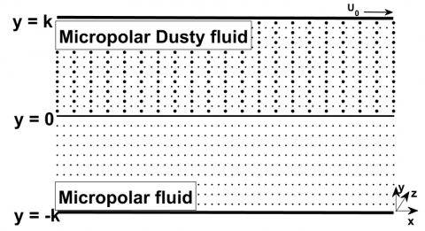
Figure 1. Geometric configuration of problem
Consider the time-dependent, Couette flow of two immiscible, incompressible micropolar and micropolar dusty fluids through a horizontal channel. The flow is unidirectional and induced by upper plate movement which is applied in the x-direction of the channel as depicted in Figure 1. Both plates are electrically non-conductive and are located in the X-Z plane and both fluids are assumed to be electrically conductive having electrical conductivity $\sigma_{C}$. An external uniform magnetic field Bu is applied on fluids in the y-axis. The lower plate is fixed and located at $y=-k$, with constant heat temperature Th1 while the upper plates at $y=k$, has the temperature Th2 and moving with constant velocity U0 Micropolar fluid filled in the lower zone of the channel i. e. ($-k \leq y \leq 0$) and owns the fluid velocity U1 Microrotation (angular velocity) N1, density $\rho_{1}$, viscosity $\mu_{1}$, vortex viscosity V1, gyro-viscosities $G_{v 1}$ and $\beta_{1}$ gyration parameter i1, thermal conductivity K1, specific heat capacity CP1 and, Micropolar dusty fluid flows in the upper zone of the channel ($0 \leq y \leq k$) and has the fluid velocity U2 Microrotation (angular velocity) N2 density $\rho_{2}$, viscosity $\mu_{2}$, vortex viscosity V2, gyro-viscosities $G_{v 2}$ and $\beta_{2}$ gyration parameter i2, thermal conductivity K2, specific heat capacity CP2. Body forces and body couples are ignored. The transportation features are similar in both domains. Let the fluid velocity $U_{i}=U_{i}(y, t)$, micro-rotation vector $N_{i}=N_{i}(y, t)$, temperature vector $T_{i}=T_{i}(y, t)$ in both regions (i=1,2) and particle velocity is $U_{p}(y, t)$ in zone II (upper). Through the mechanism of momentum exchange, the fluid layers are mechanically linked. Continuity in velocity and shear stress over the contact allows momentum to be transferred. At the interface between two fluids, moreover, we assume that the flow rate and shear pressure are also continuous. Since the fluids are electrically conducting, magnetohydrodynamic effects are caused. The channel's walls are thought to be electrically shielded. The effect of an applied transverse magnetic field on both plates, which causes stiffness in the fluid flow through the Lorentz force, which appears to drag fluid velocities written as follows [22]:
$J_{0} \times B_{u}=\frac{\sigma B_{u}^{2}(1+B i . B e) U_{i}}{(1+B i . B e)^{2}+B e^{2}}$ (1)
where, J0 is current density, Bu is the external magnetic field, $\sigma_{c}$ is the electric conductivity and Bi is the ion slip parameter, Be is the hall parameter.
Dust particles in the micropolar dusty (upper zone) fluid are uniform size, mass, non-deformable, and uniformly dispersed within the fluid. In the dusty fluid, the dust particles have particle velocity Up, density $\rho_p$, and possess the average mass mp, particle volume fraction function $\emptyset $. It’s expected that the particle phase is diluted enough that couplings between any two particles are neglected, and that the dust particle size (radius r) is small. Hence the net dust effect on the fluid particles is equivalent to the additional force per unit volume, written as [17, 22].
$\operatorname{Drag}_{f}=K N\left(U_{2}-U_{p}\right)$ (2)
Here $K=6 \pi r \mu_{2} U_{0}$ is the Stokes drag coefficient, N is the density number of a dust particle, $\mu_{2}$ is the viscosity of the micropolar dusty fluid.
Dust particles gain heat from the fluid by conduction through their surface. Let cp is the specific heat capacity of the particles, the heat conduction between the fluid and particles depends on the temperature relaxation parameter $\gamma_{\text {Temp }}$ [17, 19, 22].
$\gamma_{\text {Temp }}=\frac{3}{2} \frac{\rho_{p} \cdot c_{p} \cdot \mu_{2}}{K . N \cdot K_{2}}$ (3)
Fluid velocities $\left(U_{1}, U_{2}\right)$ particle velocity (Up), micro-rotation $\left(N_{1}, N_{2}\right)$ and temperature $\left(T_{1}, T_{2}\right)$ particle temperature (Tp), distribution of MHD (magnetohydrodynamic) flow under the aforesaid assumed constraints take the form [17, 19, 22, 25].
Zone-I (Micropolar fluid: −k ≤ y ≤ 0).
$\rho_{1} \frac{\partial U_{1}}{\partial t}=V_{1} \frac{\partial N_{1}}{\partial y}+\left(\mu_{1}+V_{1}\right) \frac{\partial^{2} U_{1}}{\partial y^{2}}-\frac{\sigma B_{u}{ }^{2}(1+B i . B e)}{(1+B i . B e)^{2}+B e^{2}} U_{1}$ (4)
$\rho_{1} i_{1} \frac{\partial N_{1}}{\partial t}=G_{v 1} \frac{\partial^{2} N_{1}}{\partial y^{2}}-V_{1}\left(2 N_{1}+\frac{\partial U_{1}}{\partial y}\right)$ (5)
$\rho_{1} C_{P 1} \frac{\partial T_{1}}{\partial t}=K_{1} \frac{\partial^{2} T_{1}}{\partial y^{2}}+\mu_{1}\left(\frac{\partial U_{1}}{\partial y}\right)^{2}+V_{1}\left(2 N_{1}+\frac{\partial U_{1}}{\partial y}\right)^{2}$
$+\beta_{1}\left(\frac{\partial N_{1}}{\partial y}\right)^{2}+\frac{\sigma B_{u}{ }^{2}(1+B i . B e)}{(1+B i . B e)^{2}+B e^{2}} U_{1}^{2}$ (6)
Zone-II (Micropolar dusty fluid: 0 ≤ y ≤ k)
$\rho_{2} \frac{\partial U_{2}}{\partial t}=V_{2} \frac{\partial N_{2}}{\partial y}+\left(\mu_{2}+V_{2}\right) \frac{\partial^{2} U_{2}}{\partial y^{2}}$
$-\frac{\sigma B_{u}{ }^{2}(1+B i . B e)}{(1+B i . B e)^{2}+B e^{2}} U_{2}-N \emptyset \frac{\left(U_{2}-U_{p}\right)}{(1-\emptyset)}$ (7)
$m_{p} \frac{\partial U_{p}}{\partial t}=K N\left(U_{2}-U_{p}\right)$ (8)
$\rho_{2} j_{2} \frac{\partial N_{2}}{\partial t}=G_{v 2} \frac{\partial^{2} N_{2}}{\partial y^{2}}-\kappa_{2}\left(2 N_{2}+\frac{\partial U_{2}}{\partial y}\right)$ (9)
$\rho_{2} C_{P 2} \frac{\partial T_{2}}{\partial t}=K_{2} \frac{\partial^{2} T_{2}}{\partial y^{2}}+\mu_{2}\left(\frac{\partial U_{2}}{\partial y}\right)^{2}+V_{2}\left(2 N_{2}+\frac{\partial U_{2}}{\partial y}\right)^{2}+\beta_{2}\left(\frac{\partial N_{2}}{\partial y}\right)^{2}+\frac{\sigma B_{u}^{2}(1+B i . B e)}{(1+B i . B e)^{2}+B e^{2}} U_{2}^{2}$
$+\frac{\rho_{p} c_{p} \emptyset\left(T_{p}-T_{2}\right)}{\gamma_{T e m p}(1-\emptyset)}+K N \rho_{p} \emptyset \frac{\left(U_{2}-U_{p}\right)^{2}}{(1-\emptyset)}$ (10)
$\frac{\partial T_{p}}{\partial t}=-\frac{\left(T_{p}-T_{2}\right)}{\gamma_{T e m p}}$ (11)
Both velocity $\left(U_{1}, U_{2}\right)$ and microrotation $\left(N_{1}, N_{2}\right)$ diminish at the duct wall whereas velocities $U_{1}$ and $U_{2}$, angular velocities $N_{1}, N_{2}$, temperature $\left(T_{1}, T_{2}\right)$ vectors, shear stress, and coupling stress are continuous at the liquid-liquid interface. Initially, the fluids and plates are maintained at a constant temperature. The temperatures on both plates are set to $T_{h 1}$ and $T_{h 2}$, respectively.
Initial conditions:
$A t t \leq 0, \quad$ and $-k \leq y \leq 0$
$\left.\begin{array}{l}U_{1}(y, t)=0 \\ N_{1}(y, t)=0 \\ T_{1}(y, t)=T_{0}\end{array}\right\}$ (12)
At $t \leq 0, \quad$ and $0 \leq y \leq k$
$\left.\begin{array}{l}U_{2}(y, t)=0 \\ N_{2}(y, t)=0 \\ T_{2}(y, t)=T_{0} \\ U_{p}(y, t)=0 \\ T_{p}(y, t)=T_{0}\end{array}\right\}$ (13)
Boundary (At channel walls) conditions: At t > 0,
$\left.\begin{array}{c}U_{1}(-k, t)=0 \\ N_{1}(-k, t)=0 \\ T_{1}(-k, t)=T_{h 1} \\ U_{2}(k, t)=U_{0} \\ U_{p}(k, t)=U_{0} \\ N_{2}(k, t)=0 \\ T_{2}(k, t)=T_{h 2} \\ T_{p}(k, t)=T_{h 2}\end{array}\right\}$ (14)
Interface conditions at y = 0.
$\left.\begin{array}{rl}U_{1}(0, t) & =U_{2}(0, t) \\ N_{1}(0, t) & =N_{2}(0, t) \\ T_{1}(0, t) & =T_{2}(0, t) \\ K_{1} T_{1 y} & =K_{2} T_{2} y \\ \left(\mu_{1}+\kappa_{1}\right) U_{1_{y}}+\kappa_{1} N_{1} & =\left(\mu_{2}+\kappa_{2}\right) U_{2_{y}}+\kappa_{2} N_{2}\end{array}\right\}$ (15)
Introducing the non-dimensional parameters:
$\left.\begin{array}{c}\bar{x}=\frac{x}{k}, \bar{y}=\frac{y}{k}, \overline{U_{1}}=\frac{U_{1}}{U_{0}}, \overline{U_{2}}=\frac{U_{2}}{U_{0}} \\ \overline{U_{p}}=\frac{U_{p}}{U_{0}}, \bar{p}=\frac{p}{\rho_{1} U_{0}^{2}}, \bar{t}=\frac{t U_{0}}{k} \\ \bar{T}_{1}=\frac{T_{1}-T_{h 1}}{T_{h 2}-T_{h 1}}, \overline{T_{2}}=\frac{T_{2}-T_{h 2}}{T_{h 2}-T_{h 1}}, \text { and } \overline{T_{p}}=\frac{T_{p}-T_{h 2}}{T_{h 2}-T_{h 1}} \\ \overline{N_{1}}=\frac{N_{1} k}{U_{0}}, \text { and } \overline{N_{2}}=\frac{N_{2} k}{U_{0}} \\ R e=\frac{\rho_{1} U_{0}}{\mu_{1}}, \quad \eta_{1}=\frac{V_{1}}{\mu_{1}}, \text { and } \eta_{2}=\frac{V_{2}}{\mu_{2}} \\ H a^{2}=\frac{\sigma B_{0}^{2} k^{2}}{\mu_{1}}, \text { and } P r=\frac{\mu_{1} C_{P 1}}{K_{1}} \\ E c=\frac{U_{0}}{C_{P 1}\left(T_{h 2}-T_{h 1}\right)}, R=\frac{K N k^{2} \emptyset}{\mu_{2}(1-\emptyset)} \\ \delta_{1}=\frac{\beta_{1}}{\mu_{1} k^{2}}, \delta_{2}=\frac{\beta_{2}}{\mu_{2} k^{2}}, r_{1}=\frac{\mu_{2}}{\mu_{1}}, r_{2}=\frac{\rho_{2}}{\rho_{1}} \\ r_{3}=\frac{\rho_{2}}{\rho_{p}}, C_{r}=\frac{C_{P 2}}{C_{P 1}}, K_{r}=\frac{K_{2}}{K_{1}}, C_{P r}=\frac{C_{P 2}}{c_{p}}\end{array}\right\}$ (16)
Assuming $\gamma_{1}=\left(\mu_{1}+V_{1} / 2\right) i_{1}$ and $\gamma_{2}=\left(\mu_{2}+V_{2} / 2\right) i_{2}$ with $i_{1}=i_{2}=k^{2}$ according to [24].
After dropping the bars, the Eqns. (3)-(9) can be written as:
Zone-I (Micropolar fluid: −k ≤ y ≤ 0).
$\frac{\partial U_{1}}{\partial t}=\frac{1}{R e}\left[\begin{array}{c}\eta_{1} \frac{\partial N_{1}}{\partial y}+\left(1+\eta_{1}\right) \frac{\partial^{2} U_{1}}{\partial y^{2}} \\ -\frac{H a^{2}(1+B i . B e)}{(1+B i . B e)^{2}+B e^{2}} U_{1}\end{array}\right]$ (17)
$\frac{\partial N_{1}}{\partial t}=\frac{1}{R e}\left[\left(1+\frac{\eta_{1}}{2}\right) \frac{\partial^{2} N_{1}}{\partial y^{2}}-\eta_{1}\left(2 N_{1}+\frac{\partial U_{1}}{\partial y}\right)\right]$ (18)
$\frac{\partial T_{1}}{\partial t}=\frac{E c}{R e}\left[\frac{1}{P r \cdot E c} \frac{\partial^{2} T_{1}}{\partial y^{2}}+\left(\frac{\partial U_{1}}{\partial y}\right)^{2}+\eta_{1}\left(2 N_{1}+\frac{\partial U_{1}}{\partial y}\right)^{2}+\delta_{1}\left(\frac{\partial N_{1}}{\partial y}\right)^{2} \frac{H a^{2}(1+B i . B e)}{(1+B i . B e)^{2}+B e^{2}} U_{1}^{2}\right]$ (19)
Zone-II (Micropolar dusty fluid: 0 ≤ y ≤ k)
$\frac{\partial U_{2}}{\partial t}=\frac{r_{1}}{r_{2} \cdot \operatorname{Re}}\left[\begin{array}{c}\eta_{2} \frac{\partial N_{2}}{\partial y}+\left(1+\eta_{2}\right) \frac{\partial^{2} U_{2}}{\partial y^{2}}- \\ \frac{H a^{2}(1+B i . B e)}{r_{1}\left((1+B i . B e)^{2}+B e^{2}\right)} U_{2}-R\left(U_{2}-U_{p}\right)\end{array}\right]$ (20)
$\frac{\partial U_{p}}{\partial t}=\frac{R \cdot r_{1} \cdot r_{3}}{r_{2} \cdot R e}\left(U_{2}-U_{p}\right)$ (21)
$\frac{\partial N_{2}}{\partial t}=\frac{r_{1}}{r_{2} \cdot R e}\left[\left(1+\frac{\eta_{2}}{2}\right) \frac{\partial^{2} N_{2}}{\partial y^{2}}-\eta_{2}\left(2 N_{2}+\frac{\partial U_{2}}{\partial y}\right)\right]$ (22)
$\frac{\partial T_{2}}{\partial t}=\frac{E c . r_{1}}{\operatorname{Re} \cdot r_{2} \cdot C_{r}}\left[\begin{array}{c}\frac{K r}{P r \cdot E c \cdot r_{1}} \frac{\partial^{2} T_{2}}{\partial y^{2}}+\left(\frac{\partial U_{2}}{\partial y}\right)^{2}+\eta_{2}\left(2 N_{2}+\frac{\partial U_{2}}{\partial y}\right)^{2}+ \\ \delta_{2}\left(\frac{\partial N_{2}}{\partial y}\right)^{2}+\frac{H a^{2}(1+B i . B e)}{r_{1}\left((1+B i . B e)^{2}+B e^{2}\right)} U_{2}^{2} \\ +\frac{2}{3} \frac{R \cdot K_{r}}{P r . E c \cdot r_{1}}\left(T_{p}-T_{2}\right)+\frac{R \cdot C_{r} \cdot r_{3}}{E c}\left(U_{2}-U_{p}\right)^{2}\end{array}\right]$ (23)
$\frac{\partial T_{p}}{\partial t}=\frac{2}{3} \frac{R * k_{r} * C_{r} * r_{3}}{C_{P r} * r_{1} * \operatorname{Pr}} \frac{\left(T_{2}-T_{p}\right)}{R e}$ (24)
Eqns. (12)-(15) are considered as initial, interfacial, and boundary conditions with $T_{0}=0, T_{h 1}=0, T_{h 2}=1, U_{0}=1$, and $k=1$.
To analyze the fluid velocity and temperature distribution for schemes I and II, the domain [-1, 1] is split into [-1, 0] for pure fluid (region –I) and [0, 1] for dusty fluid (region-II). Next both domains are likewise discretized with step length h in the y-(transverse) direction and k’ in the time scales. Similarly, the domain [-1, 1] is uniformly discretized for flow analysis for scheme III. The nodes are presumed to disperse uniformly.
$a=y_{1}<y_{2}<\cdots<y<y_{n}=b$, such that $y_{i+1}-y_{i}=h$ on the real axis. (25)
Following this, let the $R_{i_{y}}\left(y_{i}, t\right)$ is the first and $R_{i_{y y}}\left(y_{i}, t\right)$ are the second-order derivatives of $U_{1}(y, t), U_{2}(y, t), U_{P}(y, t), N_{1}(y, t), N_{2}(y, t) T_{1}(y, t), T_{2}(y, t)$ and $T_{P}(y, t)$ are obtained at any time on the nodes yi.
For $i=1,2,3, \ldots, n . U_{1_{ y}}\left(y_{i}, t\right)=\sum_{j=1}^{N} X_{i j}^{*} U_{1}\left(y_{j}, t\right)$ (26)
$U_{1_{ y y}}\left(y_{i}, t\right)=\sum_{i=1}^{N} Y^{*} U_{1}\left(y_{j}, t\right)$ (27)
For $i=1,2,3, \ldots, n . U_{2_{ y}}\left(y_{i}, t\right)=\sum_{j=1}^{N} X_{i j}^{*} U_{2}\left(y_{j}, t\right)$ (28)
$U_{2_{ y y}}\left(y_{i}, t\right)=\sum_{j=1}^{N} Y_{i j}^{*} U_{2}\left(y_{j}, t\right)$ (29)
For $i=1,2,3, \ldots, n \cdot U_{p_{y}}\left(y_{i}, t\right)=\sum_{j=1}^{N} X_{i j}^{*} U_{p}\left(y_{j}, t\right)$ (30)
$U_{p_{y y}}\left(y_{i}, t\right)=\sum_{j=1}^{N} Y^{*}{ }_{i j} U_{p}\left(y_{j}, t\right)$ (31)
For $i=1,2,3, \ldots, n . N_{1_{ y}}\left(y_{i}, t\right)=\sum_{j=1}^{N} X^{*}{ }_{i j} N_{1}\left(y_{j}, t\right)$ (32)
$N_{1_{ y y}}\left(y_{i}, t\right)=\sum_{j=1}^{N} Y_{i j}^{*} N_{1}\left(y_{j}, t\right)$ (33)
For $i=1,2,3, \ldots, n . N_{2 _{y}}\left(y_{i}, t\right)=\sum_{j=1}^{N} X_{i j}^{*} N_{2}\left(y_{j}, t\right)$ (34)
$N_{2_{ y y}}\left(y_{i}, t\right)=\sum_{i=1}^{N} Y_{i j}^{*} N_{2}\left(y_{j}, t\right)$ (35)
For $i=1,2,3, \ldots, n . T_{1_{y}}\left(y_{i}, t\right)=\sum_{j=1}^{N} X_{i j}^{*} T_{1}\left(y_{j}, t\right)$ (36)
$T_{1_{ y y}}\left(y_{i}, t\right)=\sum_{j=1}^{N} Y_{i j}^{*} T_{1}\left(y_{j}, t\right)$ (37)
For $i=1,2,3, \ldots, n . T_{2_{ y}}\left(y_{i}, t\right)=\sum_{j=1}^{N} X_{i j}^{*} T_{2}\left(y_{j}, t\right)$ (38)
$T_{2_{ y y}}\left(y_{i}, t\right)=\sum_{i=1}^{N} Y^{*}{ }_{i j} T_{2}\left(y_{j}, t\right)$ (39)
For $i=1,2,3, \ldots, n \cdot T_{p_{y}}\left(y_{i}, t\right)=\sum_{j=1}^{N} X_{i j}^{*} T_{p}\left(y_{j}, t\right)$ (40)
$T_{p_{y y}}\left(y_{i}, t\right)=\sum_{j=1}^{N} Y^{*}{ }_{i j} T_{p}\left(y_{j}, t\right)$ (41)
Here $X^{*}{ }_{i j} Y^{*}{ }_{i j}$ are the respective weighting coefficients of 1st and 2nd order derivative coefficients concerning y-coordinate, measured using modified cubic B-spline functions. The cubic B-spline functions of the knots are as specified below.
$\theta_{j}=\frac{1}{h^{3}}\left\{\begin{array}{cc}\left(y-y_{j-2}\right)^{3}, & y \epsilon\left[y_{j-2}, y_{j-1}\right) \\ \left(y-y_{j-2}\right)^{3}-4\left(y-y_{j-1}\right)^{3}, &y \epsilon\left[y_{j-1}, y_{j}\right) \\ \left(y_{j+2}-y\right)^{3}-4\left(y_{j+1}-y\right)^{3}, &y \epsilon\left[y_{j}, y_{j+1}\right) \\ \left(y_{j+2}-y\right)^{3}, & y \in\left[y_{j+1}, y_{j+2}\right) \\ 0, & \text { otherwise } .\end{array}\right.$ (42)
$\theta_{j}$ with $j=0,1,2 \ldots, N+1$ forms a basis over the region [a, b].
The updated cubic B-spline functions are described in the nodes as follows.
$F_{1}(y)=\theta_{1}(y)+2 \theta_{0}(y)$ (43)
$F_{2}(y)=\theta_{2}(y)-\theta_{0}(y)$ (44)
$F_{j}(y)=\theta_{j}$, for $j=3, \ldots, N-2$ (45)
$F_{N-1}(y)=\theta_{N-1}(y)-\theta_{N+1}(y)$ (46)
$F_{N}(y)=\theta_{N}(y)+2 \theta_{N+1}(y)$ (47)
Here $\left\{F_{1} F_{2}, \ldots, F_{N}\right\}$ forms a basis over the region [a,b]. The weighting coefficients are derived using the modified cubic B-spline function. The approximation for the 1st order derivative is:
$F_{k}^{\prime}\left(y_{i}\right)=\sum_{i=1}^{N} X^{*}{ }_{i j} \theta_{k}\left(y_{j}\right) \begin{gathered}\text { for } i=1,2, \ldots, N \\ k=1,2, \ldots, N\end{gathered}$ (48)
The estimate can be provided for the first-knot point y1.
$F_{k}^{\prime}\left(y_{1}\right)=\sum_{i=1}^{N} X^{*}{ }_{1 j} \theta_{k}\left(y_{j}\right) \quad \begin{gathered}\text { for } i=1,2, \ldots, N \\ k=1,2, \ldots, N\end{gathered}$ (49)
Then the tri-diagonal system of equations is formed as
$\left[\begin{array}{ccccccccc}6 & 1 & 0 & 0 & & & & & \\ 0 & 4 & 1 & 0 & \cdots & 0 & & 0 & \\ 0 & 1 & 4 & 1 & & & & & \\ & \vdots & & 0 & \ddots & 0 & & \vdots & \\ & & & & & 1 & 4 & 1 & 0 \\ & 0 & & 0 & \cdots & 0 & 1 & 4 & 0 \\ & & & & & 0 & 0 & 1 & 6\end{array}\right]\left[\begin{array}{c}X^{*}{ }_{11} \\ X^{*}{ }_{12} \\ X^{*}{ }_{13} \\ \cdot \\ \cdot \\ \cdot \\ X^{*}{ }_{N-3} \\ X^{*}{ }_{N-2} \\ X^{*}{ }_{N-1} \\ X^{*}_{N} \end{array}\right]=\left[\begin{array}{c}-6 / h \\ 6 / h \\ 0 \\ \cdot \\ \cdot \\ \cdot \\ 0 \\ 0 \\ 0 \\ 0\end{array}\right]$ (50)
Similarly for the point, y2 we have,
$F_{k}^{\prime}\left(y_{2}\right)=\sum_{j=1}^{N} X_{2 j}^{*} \theta_{k}\left(y_{j}\right) \begin{gathered}\text { for } i=1,2, \ldots, N \\ k=1,2, \ldots, N\end{gathered}$ (51)
Then again, the tri-diagonal system of equations is formed as:
$\left[\begin{array}{ccccccccc}6 & 1 & 0 & 0 & & & & & \\ 0 & 4 & 1 & 0 & \cdots & 0 & & 0 & \\ 0 & 1 & 4 & 1 & & & & & \\ & \vdots & & 0 & \ddots & 0 & & \vdots & \\ & & & & & 1 & 4 & 1 & 0 \\ & 0 & & 0 & \cdots & 0 & 1 & 4 & 0 \\ & & & & & 0 & 0 & 1 & 6\end{array}\right]\left[\begin{array}{c}X^{*}{ }_{21} \\ X^{*}{ }_{22} \\ X^{*}{ }_{23} \\ \cdot \\ \cdot \\ \cdot \\ X^{*}{ }_{2N-3} \\ X^{*}{ }_{2N-2} \\ X^{*}{ }_{2N-1} \\ X^{*}_{2N} \end{array}\right]=\left[\begin{array}{c}-3 / h \\ 3 / h \\ 0 \\ 0 \\ \cdot \\ \cdot \\ 0 \\ 0 \\ 0 \\ 0\end{array}\right]$ (52)
We continue to find the tri-diagonal systems for the remaining yi’s and the system for last yN is given by:
$\left[\begin{array}{ccccccccc}6 & 1 & 0 & 0 & & & & & \\ 0 & 4 & 1 & 0 & \cdots & 0 & & 0 & \\ 0 & 1 & 4 & 1 & & & & & \\ & \vdots & & 0 & \ddots & 0 & & \vdots & \\ & & & & & 1 & 4 & 1 & 0 \\ & 0 & & 0 & \cdots & 0 & 1 & 4 & 0 \\ & & & & & 0 & 0 & 1 & 6\end{array}\right]\left[\begin{array}{c}X^{*}{ }_{N1} \\ X^{*}{ }_{N2} \\ X^{*}{ }_{N3} \\ \cdot \\ \cdot \\ \cdot \\ X^{*}{ }_{NN-3} \\ X^{*}{ }_{NN-2} \\ X^{*}{ }_{NN-1} \\ X^{*}_{NN} \end{array}\right]=\left[\begin{array}{c} 0 \\ 0 \\ 0 \\ 0 \\ \cdot \\ \cdot \\ 0 \\ 0 \\ -6 / h \\ 6 / h\end{array}\right]$ (53)
The solution of the above systems provides the coefficients
$X_{11}^{*}, X_{12}^{*} \ldots, X_{1 N}^{*}, X_{21}^{*}, X_{22}^{*} \ldots, X_{2 N}^{*} \ldots, X_{N 1}^{*}, X_{N 2}^{*} \ldots, X_{N N}^{*}$.
Then the values of $Y^{*}{ }_{i j}$ for $i=1,2,3 \ldots N, j=1,2,3 \ldots N$ are calculated as follows:
$\left.\begin{array}{c}Y_{i j}^{*}=2 X^{*}{ }_{i j}\left(X^{*}{ }_{i j}-\frac{1}{y_{i}-y_{j}}\right) & \text { for } i \neq j \\ Y^{*}{ }_{i i}=-\sum_{i=1, i \neq j}^{N} Y^{*}{ }_{i j} & i=j\end{array}\right\}$ (54)
The reduced system of ordinary differential equations in time, that is, represented as for i=1, 2, 3…, N.
$V_{t}=R_{m}\left(U_{1}, U_{2}, T_{1}, T_{2}, N_{1}, N_{2} U_{p}, T_{p}\right)$ (55)
The system is solved by the following strong stability preserving scheme (section 3.1).
3.1 Computation of $u_{1}, u_{2}, \mathbf{N}_{1}, N_{2}, T_{1}, T_{2}$
To obtain the velocity, micro-rotation, and temperature profiles for MHD (magnetohydrodynamic) Couette flow of micropolar and micropolar dusty fluids in the respective Zone, replace the approximation of the spatial components of the I and II order derivatives obtained by using MCB-DQM (modified cubic b-spline differential quadrature method). Hence the system of coupled partial Eqns. (17)-(24) is numerically solved with the initial and boundary conditions (12)-(15) and the linear velocities, angular velocity component (microrotation), and temperature profiles of both fluids and particles are readily obtained. The Eqns. (17)-(24) can be updated as follows:
Zone-I (Micropolar fluid: −k ≤ y ≤ 0).
$\frac{\partial U_{1}}{\partial t}=\frac{1}{R e} \cdot\left[\begin{array}{c}\eta_{1} \sum_{j=1}^{N} X^{*}{ }_{i j} N_{1}\left(y_{j}, t\right)+\left(1+\eta_{1}\right)\left(\sum_{j=1}^{N} Y^{*}{ }_{i j} U_{1}\left(y_{j}, t\right)\right) \\ -\frac{H a^{2}(1+B i . B e)}{(1+B i . B e)^{2}+B e^{2}} U_{1}\left(y_{j}, t\right)\end{array}\right]$ (56)
$\frac{\partial N_{1}}{\partial t}=\frac{1}{R e}\left[\left(1+\frac{\eta_{1}}{2}\right)\left(\sum_{j=1}^{N} Y^{*}{ }_{i j} N_{1}\left(y_{j}, t\right)\right)-\eta_{1}\left(2 N_{1}\left(y_{j}, t\right)+\sum_{j=1}^{N} X^{*}{ }_{i j} U_{1}\left(y_{j}, t\right)\right)\right]$ (57)
$\frac{\partial T_{1}}{\partial t}=\frac{E c}{R e}\left[\begin{array}{c}\frac{1}{P r . E c}\left(\sum_{j=1}^{N} Y^{*}{ }_{i j} T_{1}\left(y_{j}, t\right)\right)+\left(\sum_{j=1}^{N} X^{*}{ }_{i j} U_{1}\left(y_{j}, t\right)\right)^{2}+ \\ \eta_{1}\left(2 N_{1}\left(y_{j}, t\right)+\sum_{j=1}^{N} X^{*}{ }_{i j} U_{1}\left(y_{j}, t\right)\right)^{2}+\delta_{1}\left(\sum_{j=1}^{N} X^{*}{ }_{i j} N_{1}\left(y_{j}, t\right)\right)^{2} \\ \frac{H a^{2}(1+B i . B e)}{(1+B i . B e)^{2}+B e^{2}} U_{1}\left(y_{j}, t\right)^{2}\end{array}\right]$ (58)
Zone-II (Micropolar dusty fluid: 0 ≤ y ≤ k)
$\frac{\partial U_{2}}{\partial t}=\frac{r_{1}}{r_{2} \cdot R e}\left[\begin{array}{c}\eta_{2} \sum_{j=1}^{N} X^{*}{ }_{i j} N_{2}\left(y_{j}, t\right)+\left(1+\eta_{2}\right)\left(\sum_{j=1}^{N} Y^{*}{ }_{i j} U_{2}\left(y_{j}, t\right)\right) \\ -\frac{H a^{2}(1+B i . B e)}{r_{1}\left((1+B i . B e)^{2}+B e^{2}\right)} U_{2}\left(y_{j}, t\right)-R\left(U_{2}\left(y_{j}, t\right)-U_{p}\left(y_{j}, t\right)\right)\end{array}\right]$ (59)
$\frac{\partial U_{p}}{\partial t}=\frac{R \cdot r_{1} \cdot r_{3}}{r_{2} \cdot R e}\left[U_{2}\left(y_{j}, t\right)-U_{p}\left(y_{j}, t\right)\right]$ (60)
$\frac{\partial N_{2}}{\partial t}=\frac{r_{1}}{r_{2} \cdot R e}\left[\left(1+\frac{\eta_{2}}{2}\right)\left(\sum_{j=1}^{N} Y_{i j}^{*} N_{2}\left(y_{j}, t\right)\right)-\eta_{2}\left(2 N_{2}\left(y_{j}, t\right)+\sum_{j=1}^{N} X^{*}{ }_{i j} U_{2}\left(y_{j}, t\right)\right)\right]$ (61)
$\left.\begin{array}{l}\frac{\partial T_{2}}{\partial t}=\frac{E c \cdot r_{1}}{R e \cdot r_{2} \cdot C_{r}}\left[\begin{array}{c}\frac{K r}{P r . E c \cdot r_{1}}\left(\sum_{j=1}^{N} Y_{i j}^{*} T_{2}\left(y_{j}, t\right)\right)+\left(\sum_{j=1}^{N} X^{*}{ }_{i j} U_{2}\left(y_{j}, t\right)\right)^{2}+\eta_{2}\left(\sum_{j=1}^{N} X_{i j}^{*} U_{2}\left(y_{j}, t\right)\right) \\ +\delta_{2}\left(\sum_{j=1}^{N} X^{*}{ }_{i j} N_{2}\left(y_{j}, t\right)\right)^{2}+\frac{H a^{2}(1+B i . B e)}{r_{1}\left((1+B i . B e)^{2}+B e^{2}\right)} U_{2}\left(y_{j}, t\right)^{2}+ \\\frac{2}{3} \frac{R \cdot K_{r}}{P r . E c \cdot r_{1}}\left(T_{p}\left(y_{j}, t\right)-T_{2}\left(y_{j}, t\right)\right)+\frac{R \cdot C_{r} \cdot r_{3}}{E c}\left(U_{2}\left(y_{j}, t\right)-U_{p}\left(y_{j}, t\right)\right)^{2}\end{array}\right.^{2}\end{array}\right]$ (62)
$\frac{\partial T_{p}}{\partial t}=\frac{2}{3} \frac{R * k_{r} * C_{r} * r_{3}}{C_{P r} * r_{1} * P r} \frac{\left(T_{2}\left(y_{j}, t\right)-T_{p}\left(y_{j}, t\right)\right)}{R e}$ (63)
Thus, equations are reduced into a system of ordinary differential equations in time, that is, for i=1, 2, 3…, N, and the system is solved by the robust four-step third-order SSP RK43 [33]. The velocities and microrotation in both Zones are obtained as follows:
At first - the step for i=1,2,3…, n
Zone-I ($-\mathrm{k} \leq \mathrm{y} \leq 0$) (micropolar fluid):
$U_{1_{1}}=U_{1_{0}}+\frac{\Delta t}{2}\left(\frac{1}{R e} \cdot\left[\begin{array}{c}\eta_{1} \sum_{j=1}^{N} X_{i j}^{*} N_{1_{0}}\left(y_{j}, t\right)+ \\ \left(1+\eta_{1}\right)\left(\sum_{j=1}^{N} Y_{i j}^{*} U_{1_{0}}\left(y_{j}, t\right)\right) \\ -\frac{H a^{2}(1+B i . B e)}{(1+B i . B e)^{2}+B e^{2}} U_{1_{0}}\left(y_{j}, t\right)\end{array}\right]\right)$ (64)
$N_{1_{1}}=N_{10}+\frac{\Delta t}{2}\left(\frac{1}{R e}\left[\left(1+\frac{\eta_{1}}{2}\right)\left(\sum_{j=1}^{N} Y^{*}{ }_{i j} N_{1_{0}}\left(y_{j}, t\right)\right)-\eta_{1}\left(\begin{array}{c}2 N_{1_{0}}\left(y_{j}, t\right)+ \\ \sum_{j=1}^{N} X^{*} U_{i j} U_{1_{0}}\left(y_{j}, t\right)\end{array}\right)\right]\right)$ (65)
$\left.T_{1_{1}}=T_{1_{0}}+\frac{\Delta t}{2}\left(\begin{array}{c}\frac{E c}{R e}\left[\begin{array}{c}\frac{1}{P r . E c}\left(\sum_{j=1}^{N} Y^{*}{ }_{i j} T_{10}\left(y_{j}, t\right)\right)+\left(\sum_{j=1}^{N} X^{*}{ }_{i j} U_{10}\left(y_{j}, t\right)\right)^{2}+\eta_{1}\left(2 N_{10}\left(y_{j}, t\right)+\sum_{j=1}^{N} X^{*}{ }_{i j} U_{1_{0}}\left(y_{j}, t\right)\right)^{2} \\ +\delta_{1}\left(\sum_{j=1}^{N} X^{*}{ }_{i j} N_{1}\left(y_{j}, t\right)\right)^{2}+\frac{H a^{2}(1+B i . B e)}{(1+B i . B e)^{2}+B e^{2}} U_{1_{0}}\left(y_{j}, t\right)^{2}\end{array}\right.\end{array}\right]\right)$ (66)
Zone-II (0 ≤ y ≤ k) (micropolar dusty fluid):
$U_{2_{1}}=U_{2_{0}}+\frac{\Delta t}{2}\left(\frac{r_{1}}{r_{2} \cdot R e}\left[\begin{array}{c}\eta_{2} \sum_{j=1}^{N} X^{*}{ }_{i j} N_{2_{0}}\left(y_{j}, t\right)+\left(1+\eta_{2}\right)\left(\sum_{j=1}^{N} Y^{*}{ }_{i j} U_{2_{0}}\left(y_{j}, t\right)\right) \\ -\frac{H a^{2}(1+B i . B e)}{r_{1}\left((1+B i \cdot B e)^{2}+B e^{2}\right)} U_{2_{0}}\left(y_{j}, t\right)-R\left(U_{2_{0}}\left(y_{j}, t\right)-U_{p_{0}}\left(y_{j}, t\right)\right)\end{array}\right]\right)$ (67)
$U_{p_{1}}=U_{p_{0}}+\frac{\Delta t}{2}\left(\frac{R \cdot r_{1} \cdot r_{3}}{r_{2} \cdot R e}\left[U_{20}\left(y_{j}, t\right)-U_{p_{0}}\left(y_{j}, t\right)\right]\right)$ (68)
$N_{2_{1}}=N_{1_{0}}+\frac{\Delta t}{2}\left(\frac{r_{1}}{r_{2} \cdot \operatorname{Re}}\left[\left(1+\frac{\eta_{2}}{2}\right)\left(\sum_{j=1}^{N} Y^{*}{ }_{i j} N_{2_{0}}\left(y_{j}, t\right)\right)-\eta_{2}\left(2 N_{2_{0}}\left(y_{j}, t\right)+\sum_{j=1}^{N} X^{*}{ }_{i j} U_{2_{0}}\left(y_{j}, t\right)\right)\right]\right)$ (69)
$T_{2_{1}}=T_{1_{0}}+\frac{\Delta t}{2} \cdot\left(\frac{E c . r_{1}}{R e \cdot r_{2} \cdot C_{r}}\left[\begin{array}{c}\frac{K r}{\operatorname{Pr} . E c . r_{1}}\left(\sum_{j=1}^{N} Y^{*} T_{2_{0}}\left(y_{j}, t\right)\right)+\left(\sum_{j=1}^{N} X^{*}{ }_{i j} U_{2_{0}}\left(y_{j}, t\right)\right)^{2} \\ +\eta_{2}\left(2 N_{2_{0}}\left(y_{j}, t\right)+\sum_{j=1}^{N} X^{*}{ }_{i j} U_{2_{0}}\left(y_{j}, t\right)\right)^{2}+ \\ \delta_{2}\left(\sum_{j=1}^{N} X^{*}{ }_{i j} N_{2_{0}}\left(y_{j}, t\right)\right)^{2}+\frac{H a^{2}(1+B i . B e)}{r_{1}\left((1+B i . B e)^{2}+B e^{2}\right)} U_{2_{0}}\left(y_{j}, t\right)^{2} \\ +\frac{2}{3} \frac{R \cdot K_{r}}{P r . E c \cdot r_{1}}\left(T_{p_{0}}\left(y_{j}, t\right)-T_{2_{0}}\left(y_{j}, t\right)\right)+\frac{R \cdot C_{r} \cdot r_{3}}{E c}\left(U_{2_{0}}\left(y_{j}, t\right)-U_{p_{0}}\left(y_{j}, t\right)\right)^{2}\end{array}\right]\right)$ (70)
$T_{p_{1}}=T_{p_{0}}+\frac{\Delta t}{2}\left(\frac{2}{3} \frac{R * k_{r} * C_{r} * r_{3}}{C_{P r} * r_{1} * \operatorname{Pr}} \frac{\left(T_{2_{0}}\left(y_{j}, t\right)-T_{p_{0}}\left(y_{j}, t\right)\right)}{R e}\right)$ (71)
At the first step of the method, the conditions (12)-(15) are regarded favourably.
At the second step for i=1,2,3…, n:
Zone-I ($-k \leq y \leq 0$) (micropolar fluid):
$\begin{gathered}
U_{1_{2}}=U_{1_{1}}+ \\
\frac{\Delta t}{2}\left(\frac{1}{R e} \cdot\left[\begin{array}{c}
\eta_{1} \sum_{j=1}^{N} X^{*}{ }_{i j} N_{1_{1}}\left(y_{j}, t\right)+ \\
\left(1+\eta_{1}\right)\left(\sum_{j=1}^{N} Y^{*}{ }_{i j} U_{1_{1}}\left(y_{j}, t\right)\right) \\
-\frac{H a^{2}(1+B i . B e)}{(1+B i \cdot B e)^{2}+B e^{2}} U_{1_{1}}\left(y_{j}, t\right)
\end{array}\right]\right)
\end{gathered}$ (72)
$N_{12}=N_{11}+\frac{\Delta t}{2}\left(\frac{1}{R e}\left[\left(1+\frac{\eta_{1}}{2}\right)\left(\sum_{j=1}^{N} Y^{*}{ }_{i j} N_{1_{1}}\left(y_{j}, t\right)\right)-\eta_{1}\left(2 N_{1_{1}}\left(y_{j}, t\right)+\sum_{j=1}^{N} X_{i j}^{*} U_{1_{1}}\left(y_{j}, t\right)\right)\right]\right)$ (73)
$\left.T_{1_{2}}=T_{1_{1}}+\frac{\Delta t}{2}\left(\begin{array}{c}\frac{E c}{R e}\left[\begin{array}{c}\frac{1}{P r . E c}\left(\sum_{j=1}^{N} Y^{*}{ }_{i j} T_{1_{1}}\left(y_{j}, t\right)\right)+\left(\sum_{j=1}^{N} X^{*}{ }_{i j} U_{1_{1}}\left(y_{j}, t\right)\right)^{2}+ \\ \eta_{1}\left(2 N_{1_{1}}\left(y_{j}, t\right)+\sum_{j=1}^{N} X^{*}{ }_{i j} U_{1_{1}}\left(y_{j}, t\right)\right)^{2}+\delta_{1}\left(\sum_{j=1}^{N} X^{*}{ }_{i j} N_{1_{1}}\left(y_{j}, t\right)\right)^{2} \\ \frac{H a^{2}(1+B i . B e)}{(1+B i . B e)^{2}+B e^{2}} U_{1_{1}}\left(y_{j}, t\right)^{2}\end{array}\right.\end{array}\right]\right)$ (74)
Zone-II (0 ≤ y ≤ k) (micropolar dusty fluid):
$U_{2_{2}}=U_{2_{1}}+\frac{\Delta t}{2}\left(\frac{r_{1}}{r_{2} \cdot R e}\left[\begin{array}{c}\eta_{2} \sum_{j=1}^{N} X^{*}{ }_{i j} N_{2_{1}}\left(y_{j}, t\right)+\left(1+\eta_{2}\right)\left(\sum_{j=1}^{N} Y^{*}{ }_{i j} U_{2_{1}}\left(y_{j}, t\right)\right) \\ -\frac{H a^{2}(1+B i . B e)}{r_{1}\left((1+B i . B e)^{2}+B e^{2}\right)} U_{2_{1}}\left(y_{j}, t\right)-R\left(U_{2_{1}}\left(y_{j}, t\right)-U_{p_{1}}\left(y_{j}, t\right)\right)\end{array}\right]\right)$ (75)
$U_{p_{2}}=U_{p_{1}}+\frac{\Delta t}{2}\left(\frac{R \cdot r_{1} \cdot r_{3}}{r_{2} \cdot \operatorname{Re}}\left[U_{21}\left(y_{j}, t\right)-U_{p_{1}}\left(y_{j}, t\right)\right]\right)$ (76)
$N_{22}=N_{11}+\left(\frac{r_{1}}{r_{2} \cdot R e}\left[\left(1+\frac{\eta_{2}}{2}\right)\left(\sum_{j=1}^{N} Y^{*}{ }_{i j} N_{21}\left(y_{j}, t\right)\right)-\eta_{2}\left(\begin{array}{c}2 N_{2_{1}}\left(y_{j}, t\right)+ \\ \sum_{j=1}^{N} X^{*}{ }_{i j} U_{21}\left(y_{j}, t\right)\end{array}\right)\right]\right)$ (77)
$\left.T_{2_{2}}=T_{1_{1}}+\frac{\Delta t}{2} \cdot\left(\frac{E c \cdot r_{1}}{\text { Re. } r_{2} \cdot C_{r}} \left[ \begin{array}{ccc} \frac{K r}{P r . E c \cdot r_{1}}\left(\sum_{j=1}^{N} Y^{*}{ }_{i j} T_{2_{1}}\left(y_{j^{\prime}} t\right)\right)+\left(\sum_{j=1}^{N} X^{*}{ }_{i j} U_{2_{1}}\left(y_{j^{\prime}}, t\right)\right)^{2}+\eta_{2}\left(2 N_{21}\left(y_{j^{\prime}}, t\right)+\sum_{j=1}^{N} X^{*}{ }_{i j} U_{2_{1}}\left(y_{j^{\prime}}, t\right)\right)^{2} \\ +\delta_{2}\left(\sum_{j=1}^{N} X^{*}{ }_{i j} N_{21}\left(y_{j^{\prime}}, t\right)\right)^{2}+\frac{H a^{2}(1+B i . B e)}{r_{1}\left((1+B i . B e)^{2}+B e^{2}\right)} U_{21}\left(y_{j^{\prime}}, t\right)^{2}\\+\frac{2}{3} \frac{R \cdot K_{r}}{P r \cdot E c \cdot r_{1}}\left(T_{p_{1}}\left(y_{j^{\prime}}, t\right)-T_{2_{1}}\left(y_{j^{\prime}}, t\right)\right)+\frac{R \cdot C_{r} \cdot r_{3}}{E c}\left(U_{21}\left(y_{j^{\prime}} t\right)-U_{p_{1}}\left(y_{j}, t\right)\right)^{2} \end{array}\right] \right]\right)$ (78)
$T_{p_{2}}=T_{p_{1}}+\frac{\Delta t}{2}\left(\frac{2}{3} \frac{R * k_{r} * C_{r} * r_{3}}{C_{P r} * r_{1} * \operatorname{Pr}} \frac{\left(T_{21}\left(y_{j}, t\right)-T_{p_{1}}\left(y_{j}, t\right)\right)}{\operatorname{Re}}\right)$ (79)
At the second step of the method, the conditions (12)-(15) are regarded favourably.
At the third step for i=1,2,3…,n
Zone-I ( $-k \leq y \leq 0$) (micropolar fluid):
$U_{1_{3}}=\frac{2 . U_{1_{0}}}{3}+\frac{U_{1_{1}}}{3}+\frac{\Delta t}{6}\left(\frac{1}{R e} \cdot\left[\begin{array}{c}\eta_{1} \sum_{j=1}^{N} X^{*}{ }_{i j} N_{1_{2}}\left(y_{j}, t\right)+ \\ \left(1+\eta_{1}\right)\left(\sum_{j=1}^{N} Y^{*}{ }_{i j} U_{1_{2}}\left(y_{j}, t\right)\right) \\ -\frac{H a^{2}(1+B i . B e)}{(1+B i \cdot B e)^{2}+B e^{2}} U_{1_{2}}\left(y_{j}, t\right)\end{array}\right]\right)$ (80)
$N_{1_{3}}=\frac{2 . N_{1_{0}}}{3}+\frac{N_{1_{1}}}{3}+\frac{\Delta t}{6}\left(\frac{1}{R e}\left[\begin{array}{c}\left(1+\frac{\eta_{1}}{2}\right)\left(\sum_{j=1}^{N} Y^{*}{ }_{i j} N_{12}\left(y_{j}, t\right)\right) \\ -\eta_{1}\left(\begin{array}{c}2 N_{12}\left(y_{j}, t\right)+ \\ \sum_{j=1}^{N} X^{*}{ }_{i j} U_{12}\left(y_{j}, t\right)\end{array}\right)\end{array}\right]\right)$ (81)
$T_{1_{3}}=\frac{2 . T_{1_{0}}}{3}+\frac{T_{1_{1}}}{3}+\frac{\Delta t}{6}\left(\begin{array}{c}\left.\frac{E c}{R e}\left[\begin{array}{c}\frac{1}{P r . E c}\left(\sum_{j=1}^{N} Y_{i j}^{*} T_{12}\left(y_{j}, t\right)\right)+\left(\sum_{j=1}^{N} X_{i j}^{*} U_{12}\left(y_{j}, t\right)\right)^{2}+ \\ \eta_{1}\left(2 N_{1_{2}}\left(y_{j}, t\right)+\sum_{j=1}^{N} X^{*}{ }_{i j} U_{1_{2}}\left(y_{j}, t\right)\right)^{2} \\ +\delta_{1}\left(\sum_{j=1}^{N} X^{*}{ }_{i j} N_{1_{2}}\left(y_{j}, t\right)\right)^{2}+\frac{H a^{2}(1+B i . B e)}{(1+B i . B e)^{2}+B e^{2}} U_{1_{2}}\left(y_{j}, t\right)^{2}\end{array}\right]\right)\end{array}\right.$ (82)
Zone-II (0 ≤ y ≤ k) (micropolar dusty fluid):
$U_{2_{3}}=\frac{2 . U_{2_{0}}}{3}+\frac{U_{2_{1}}}{3}+\frac{\Delta t}{6}\left(\frac{r_{1}}{r_{2} \cdot R e}\left[\begin{array}{c}\eta_{2} \sum_{j=1}^{N} X^{*}{ }_{i j} N_{2_{2}}\left(y_{j}, t\right)+\left(1+\eta_{2}\right)\left(\sum_{j=1}^{N} Y^{*}{ }_{i j} U_{2_{2}}\left(y_{j}, t\right)\right) \\ -\frac{H a^{2}(1+B i . B e)}{r_{1}\left((1+B i, B e)^{2}+B e^{2}\right)} U_{2_{2}}\left(y_{j}, t\right)-R\left(U_{2_{2}}\left(y_{j}, t\right)-U_{p_{2}}\left(y_{j}, t\right)\right)\end{array}\right]\right)$ (83)
$U_{p_{3}}=\frac{2 . U_{p_{0}}}{3}+\frac{U_{p_{1}}}{3}+\frac{\Delta t}{6}\left(\frac{R \cdot r_{1} \cdot r_{3}}{r_{2}, R e}\left[U_{22}\left(y_{j}, t\right)-U_{p_{2}}\left(y_{j}, t\right)\right]\right)$ (84)
$N_{2_{3}}=\frac{2 . N_{2_{0}}}{3}+\frac{N_{2_{1}}}{3}+\frac{\Delta t}{6}\left(\frac{r_{1}}{r_{2} \cdot R e}\left[\left(1+\frac{\eta_{2}}{2}\right)\left(\sum_{j=1}^{N} Y^{*}{ }_{i j} N_{2_{2}}\left(y_{j}, t\right)\right)-\eta_{2}\left(\begin{array}{c}2 N_{2_{2}}\left(y_{j}, t\right)+ \\ \sum_{j=1}^{N} X_{i j}^{*} U_{2}\left(y_{j}, t\right)\end{array}\right)\right]\right)$ (85)
$T_{2_{3}}=\frac{2 \cdot T_{2}}{3}+\frac{T_{2_{1}}}{3}+\frac{\Delta t}{6} \cdot\left(\frac{E c \cdot r_{1}}{R e \cdot r_{2} \cdot C_{r}} \left[\begin{array}{c}\frac{K r}{P r . E c \cdot r_{1}}\left(\sum_{j=1}^{N} Y^{*}{ }_{i j} T_{2_{2}}\left(y_{j}, t\right)\right)+\left(\sum_{j=1}^{N} X^{*}{ }_{i j} U_{2_{2}}\left(y_{j}, t\right)\right)^{2} \\ +\eta_{2}\left(2 N_{2_{2}}\left(y_{j}, t\right)+\sum_{j=1}^{N} X^{*}{ }_{i j} U_{2_{2}}\left(y_{j}, t\right)\right)^{2}+ \\ \delta_{2}\left(\sum_{j=1}^{N} X^{*}{ }_{i j} N_{2_{2}}\left(y_{j}, t\right)\right)^{2}+\frac{H a^{2}(1+B i . B e)}{r_{1}\left((1+B i \cdot B e)^{2}+B e^{2}\right)} U_{2_{2}}\left(y_{j}, t\right)^{2} \\ +\frac{2}{3} \frac{R \cdot K_{r}}{P r \cdot E c \cdot r_{1}}\left(T_{p_{2}}\left(y_{j}, t\right)-T_{2_{2}}\left(y_{j}, t\right)\right)+\frac{R \cdot C_{r} r_{3}}{E c}\left(U_{2_{2}}\left(y_{j}, t\right)-U_{p_{2}}\left(y_{j}, t\right)\right)^{2}\end{array}\right] \right)$ (86)
$T_{p_{3}}=\frac{2 \cdot T_{p_{0}}}{3}+\frac{T_{p_{1}}}{3}+\frac{\Delta t}{6} \cdot\left(\frac{2}{3} \frac{R * k_{r} * C_{r} * r_{3}}{C_{P r} * r_{1} * P r} \frac{\left(T_{2_{1}}\left(y_{j}, t\right)-T_{p_{1}}\left(y_{j}, t\right)\right)}{R e}\right)$ (87)
At the third step of the method, the conditions (12)-(15) are once again regarded favourably.
At the fourth step for i=1,2,3…,n:
Zone-I ($-k \leq y \leq 0$,) (micropolar fluid):
$U_{1_{4}}=U_{1_{3}}+\frac{\Delta t}{2}\left(\frac{1}{R e} \cdot\left[\begin{array}{c}\eta_{1} \sum_{j=1}^{N} X^{*}{ }_{i j} N_{1_{3}}\left(y_{j}, t\right)+ \\ \left(1+\eta_{1}\right)\left(\sum_{j=1}^{N} Y_{i j}^{*} U_{1_{3}}\left(y_{j}, t\right)\right) \\ -\frac{H a^{2}(1+B i . B e)}{(1+B i \cdot B e)^{2}+B e^{2}} U_{1_{3}}\left(y_{j}, t\right)\end{array}\right]\right)$ (88)
$N_{1_{4}}=N_{1_{3}}+\frac{\Delta t}{2}\left(\frac{1}{R e}\left[\begin{array}{c}\left(1+\frac{\eta_{1}}{2}\right)\left(\sum_{j=1}^{N} Y^{*}{ }_{i j} N_{1_{3}}\left(y_{j}, t\right)\right) \\ -\eta_{1}\left(\begin{array}{c}2 N_{1_{3}}\left(y_{j}, t\right)+ \\ \sum_{j=1}^{N} X^{*} U_{1_{3}}\left(y_{j}, t\right)\end{array}\right)\end{array}\right]\right)$ (89)
$T_{1_{4}}=T_{1_{3}}+\frac{\Delta t}{2}\left(\frac{E c}{R e}\left[\begin{array}{c}\frac{1}{\operatorname{Pr} . E c}\left(\sum_{j=1}^{N} Y^{*}{ }_{i j} T_{13}\left(y_{j}, t\right)\right)+\left(\sum_{j=1}^{N} X^{*}{ }_{i j} U_{13}\left(y_{j}, t\right)\right)^{2}+ \\ \eta_{1}\left(2 N_{1_{3}}\left(y_{j}, t\right)+\sum_{j=1}^{N} X^{*}{ }_{i j} U_{1_{3}}\left(y_{j}, t\right)\right)^{2} \\ +\delta_{1}\left(\sum_{j=1}^{N} X^{*}{ }_{i j} N_{1_{3}}\left(y_{j}, t\right)\right)^{2}+\frac{H a^{2}(1+B i . B e)}{(1+B i . B e)^{2}+B e^{2}} U_{1_{3}}\left(y_{j}, t\right)^{2}\end{array}\right]\right)$ (90)
Zone-II (0 ≤ y ≤ k) (micropolar dusty fluid):
$U_{2_{4}}=U_{2_{3}}+\frac{\Delta t}{2}\left(\frac{r_{1}}{r_{2} \cdot R e}\left[\begin{array}{c}\eta_{2} \sum_{j=1}^{N} X_{i j}^{*} N_{2_{3}}\left(y_{j}, t\right)+ \\ \left(1+\eta_{2}\right)\left(\sum_{j=1}^{N} Y_{i j}^{*} U_{2_{3}}\left(y_{j}, t\right)\right) \\ -\frac{H a^{2}(1+B i . B e)}{r_{1}\left((1+B i \cdot B e)^{2}+B e^{2}\right)} U_{2_{3}}\left(y_{j}, t\right) \\ -R\left(U_{2_{3}}\left(y_{j}, t\right)-U_{p_{3}}\left(y_{j}, t\right)\right)\end{array}\right]\right)$ (91)
$U_{p_{4}}=U_{p_{3}}+\frac{\Delta t}{2}\left(\frac{R \cdot r_{1} \cdot r_{3}}{r_{2} \cdot R e}\left[U_{2_{3}}\left(y_{j}, t\right)-U_{p_{3}}\left(y_{j}, t\right)\right]\right)$ (92)
$N_{2_{4}}=N_{2_{3}}+\frac{\Delta t}{2}\left(\frac{r_{1}}{r_{2} \cdot R e}\left[\begin{array}{c}\left(1+\frac{\eta_{2}}{2}\right)\left(\sum_{j=1}^{N} Y^{*}{ }_{i j} N_{2}\left(y_{j}, t\right)\right) \\ -\eta_{2}\left(2 N_{2_{3}}\left(y_{j}, t\right)+\sum_{j=1}^{N} X_{i j}^{*} U_{23}\left(y_{j}, t\right)\right)\end{array}\right)\right]$ (93)
$T_{2_{4}}=T_{2_{3}}+\frac{\Delta t}{2} \cdot\left(\frac{E c \cdot r_{1}}{R e \cdot r_{2} \cdot C_{r}} \left[\begin{array}{c}\frac{K r}{P r . E c \cdot r_{1}}\left(\sum_{j=1}^{N} Y_{i j}^{*} T_{2_{3}}\left(y_{j}, t\right)\right)+\left(\sum_{j=1}^{N} X^{*}{ }_{i j} U_{23}\left(y_{j}, t\right)\right)^{2} \\ +\eta_{2}\left(2 N_{2_{3}}\left(y_{j}, t\right)+\sum_{j=1}^{N} X^{*}{ }_{i j} U_{2_{3}}\left(y_{j}, t\right)\right)^{2}+\delta_{2}\left(\sum_{j=1}^{N} X^{*}{ }_{i j} N_{2_{3}}\left(y_{j}, t\right)\right)^{2} \\ +\frac{H a^{2}(1+B i . B e)}{r_{1}\left((1+B i . B e)^{2}+B e^{2}\right)} U_{2_{3}}\left(y_{j}, t\right)^{2}+\frac{2}{3} \frac{R \cdot K_{r}}{\operatorname{Pr} \cdot \operatorname{Ec} \cdot r_{1}}\left(\begin{array}{c}T_{p_{3}}\left(y_{j}, t\right) \\ -T_{2_{3}}\left(y_{j}, t\right)\end{array}\right)+\frac{R \cdot C_{r} \cdot r_{3}}{E c}\left(\begin{array}{c}U_{2_{3}}\left(y_{j}, t\right) \\ -U_{p_{3}}\left(y_{j}, t\right)\end{array}\right)^{2}\end{array}\right] \right)$ (94)
$T_{p_{4}}=T_{p_{3}}+\frac{\Delta t}{2}\left(\frac{2}{3} \frac{R * k_{r} * C_{r} * r_{3}}{C_{P r} * r_{1} * \operatorname{Pr}} \frac{\left(T_{2_{3}}\left(y_{j}, t\right)-T_{p_{3}}\left(y_{j}, t\right)\right)}{\operatorname{Re}}\right)$ (95)
At the fourth step of the method, the conditions (12)-(15) are also regarded favourably.
Hence the fluid (linear) velocity and angular velocity (Eringen microrotation) and temperatures profiles i. e. $U_{1}, N_{1}, T_{1}$, of micropolar fluid in Zone-I, and also the fluid velocity (linear) and particle velocity components, angular velocity, and temperature profiles. $U_{2}, U_{p} N_{2}, T_{2}, T_{p}$ for micropolar dusty fluid in Zone-II can be numerically obtained at the fourth step of MCB-DQM.
3.2 Skin friction coefficient
As fluid moves over the plates, it creates friction on their edges, which inhibits forward motion and causes skin friction drift on the surface. This impact is measured using the skin friction coefficient. The expression of skin friction coefficients at both plates are calculated as
At lower plate,
$\left(\boldsymbol{C}_{f}\right)_{y=-1}=\frac{2}{\boldsymbol{R e}}\left[\left(1+\eta_{1}\right) \frac{\partial U_{1}}{\partial y}+\eta_{1} N_{1}\right]_{y=-1}$ (96)
At upper plate,
$\left(C_{f}\right)_{y=1}=\frac{2 r_{1}}{r_{2} R e}\left[\left(1+\eta_{1}\right) \frac{\partial U_{1}}{\partial y}+\eta_{1} N_{1}\right]_{y=1}$ (97)
3.3 Nusselt number
The expression of the Nusselt number at both plates is calculated as:
At lower plate,
$\left(N_{U}\right)_{y=-1}=\left(-\frac{\partial T_{1}}{\partial y}\right)_{y=-1}$ (98)
At upper plate,
$\left(N_{U}\right)_{y=1}=\left(-\frac{\partial T_{2}}{\partial y}\right)_{y=1}$ (99)
The time-dependent unidirectional Couette flow of two immiscible micropolar and micropolar-dusty fluids under magnetohydrodynamic effect and heat transfer examined. The two-fluid flow coupled problem (Eqns. (17)-(24)) in the corresponding regions with stable and continuous interface have been numerically solved by modified cubic B-spline differential quadrature method, and velocity, microrotation, and temperature profiles of fluids, and dust particles have been calculated. The analysis of skin friction coefficient and Nusselt number are also explored. The results are discussed in the following set of fixed values of all parameters, Ge=5, $t=0.5, \eta_{1}=0.5, \eta_{2}=0.5, H a^{2}=2, B e=2, B i=2$, Re=2, R=2, $r_{1}=0.5, r_{2}=0.5, r_{3}=100, C_{r}=0.5, E c=0.5, K r=0.5, \operatorname{Pr}=$$2, \delta_{1}=2, \delta_{2}=2, C r_{r}=0.5$. The simulation outputs are validated for velocity profile by comparing them with the one fluid case (the non-MHD, non-dusty, single Newtonian Couette flow $H a^{2}=0, B e=0, B i=0, R=0, \eta_{1}=0, \eta_{2}=0, \quad r_{1}=1$$r_{2}=1 G e=0$). The limiting case numerical result and the exact solution (Appendix) have a strong agreement, as seen in Figure 2.
Figure 2. Comparison of numerical solution with the exact solution
4.1 Analysis of velocity profiles
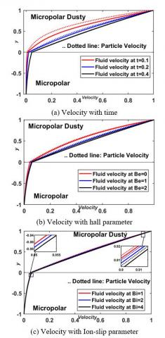
Figures 3a-3i represents the effect of various fluid parameters on fluids and particle velocity and it is cited from Figure 3a that both fluid and particle velocity increasing with time and it became stable for a higher value of time. Hall parameter $\left(B e=\sigma \beta B_{0}\right)$ and Ion-slip parameter $(B i)$ also affect the velocity but the magnitude is little less as compared to time; Hence the magnetic resistive force is decreased as Be and Bi are increased, creating an acceleration in the main flow, which increases fluid and particle-phase velocities the profile slightly and get stable for higher values (see Figure 3b and Figure 3c). If the flow is induced by constantly applied pressure from x-direction then it is known as the generalized Couette flow. The Reynold’s number $R e=\frac{\rho_{1 U_{0} h}}{\mu_{1}}$ is the non-dimensional parameter which is defined as the ratio of inertial to viscous forces. Lower viscous forces are referred to higher Re values in the fluid medium. As the Reynolds number rises, viscous forces decrease, causing an increasing correlation of fluid velocities (See Figure 3d- generalized Couette flow with Re). Figure 3e shows that if there is no external pressure on fluids then rising the Re value decreases the velocity profiles. The parameter Hartmann number $H a^{2}=\frac{\sigma B_{0}^{2} k^{2}}{\mu_{1}}$ calculates the results of a transverse magnetic field. According to Figure 3f, increasing Ha2 the allows the velocity fields in both regions to decrease. This may be attributed to the effect of an applied transverse magnetic field on both plates, which causes resistance to fluid movement through the Lorentz force, which appears to draw fluid velocities down. Increasing the micropolar parameters $\eta_{1}=\frac{\kappa_{1}}{\mu_{1}}, \eta_{2}=\frac{\kappa_{2}}{\mu_{2}}$ of both fluids, increase the vortex viscosities $\kappa_{1}$ and $\kappa_{2}$; hence the velocity profiles of the fluids and particle-phase increase slightly in respective regions (see Figure 3g, Figure 3h). Figure 3i indicates that only the dust particle velocity increases with an enhancement of particle concentration parameter R, and no variation in fluid velocities is observed.
Figure 3. The effect of various fluid parameters on velocity profiles of micropolar and micropolar dusty fluid
4.2 Analysis of micropolar profiles
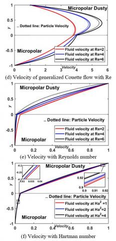
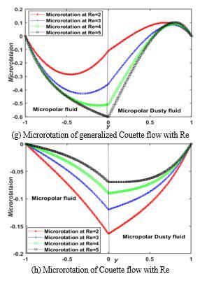
Figures 4a-4h represents the effect of various fluid parameters on microrotations (angular velocities) and it is observed from Figure 4a, that the microrotation decreasing with time and reaching a steady state after a higher value. According to Figure 4b, increasing Ha2 microrotation increase in both regions. Figure 4c and Figure 4d show that enhancing the Hall (Be) and Ion-slip parameter (Bi) decreases, microrotation in both region fluids. Figure 4e shows that increasing the micropolar parameters η1 of micropolar fluid, microrotation profiles in both regions increase slightly while profiles get significant increment with the micropolar parameters η2 of micropolar dusty fluid (see Figure 4f). Figure4g exhibits that the Microrotation profiles in both regions decrease with Reynold’s number Re when the flow is induced by constant pressure while the profiles increase with Re in the absence of applied pressure (see Figure 4h).
Figure 4. The effect of various fluid parameters on microrotation profiles of Micropolar and Micropolar dusty fluid
4.3 Analysis of temperature profiles
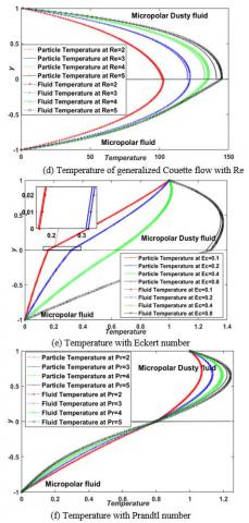
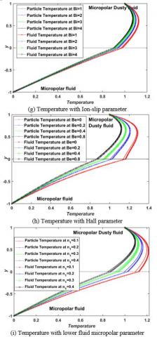
The nonlinear and flow-dependent viscous dissipation terms are not skipped during the simulation. Figure 5a to 5l exhibits the effect of various fluid parameters on heat transfer profiles of micropolar and micropolar dusty fluids and it is observed from Figure 5a, Figure 5b, Figure 5e, Figure 5j, Figure 5k and Figure 5l that the temperature profiles of both region fluids increase with time, Hartman number Ha2 (effect transverse magnetic field applied to both plates), Eckert number ( Ec- which provides the ratio of the advective mass transfer to the heat dissipation potential), the micropolar parameter of micropolar dusty fluid η2, and the ratio of viscosity r1 and density r2. The increment in the Ion-slip parameter (Bi), Hall parameter (Be) and micropolar parameter of micropolar fluid η1 cause a decline in the temperatures in both regions (see Figure 5g, Figure 5h, and Figure 5i). Figure 5c shows that if the flow is carried out by upper plate movement (Couette flow) increasing Reynold’s number Re reduces the temperature profiles in both the regions while Figure 5d shows that if the flow is carried out by constant pressure increasing Reynold’s number Re reduces the viscous force hence temperature profiles of both fluids have increasing nature. It is cited from Figure 5e, increasing the Prandtl number (Pr) which is the ratio of viscous diffusivity to thermal diffusivity, enhanced the temperature profiles of fluid and particle in the upper region, and changes its nature from increasing to decreasing in the lower region.
Figure 5. The effect of various fluid parameters on temperature profiles of Micropolar and Micropolar dusty fluid
4.4 Analysis of skin-friction coefficient
As fluid flows over the plates, the flow becomes chaotic at some point in the flow path. The existence of vortices indicates that turbulent flow has a fluctuating and unstable pattern of flow. So frictional forces are applied to the plate surface preventing fluid moves; this is known as skin friction drag. Table 1 shows that at the lower plate of the channel, skin friction increases with time (t), the micropolar parameter $\eta_{1}$ of lower region fluid, micropolar parameter η2, Hall (Be) and Ion-slip parameter (Bi). It shows a slight decrement with Reynolds number (Re), Hartman number Ha2 but remains constant with increasing values of particle concertation parameter R.
On the upper plate, the skin friction coefficient is declined by rising values of time, η1, η2, Be, and Bi. When, and Ha2 and Re increased, the co-efficient improves slightly and it does not change with R.
4.5 Analysis Nusselt number
The Nusselt number, which is equal to the dimensionless temperature gradient at the plates and is calculated at the channel wall only, is a measure of convection heat transfer at the surface. Table 2 shows that the Nusselt number increases at the upper plate and decrease at the lower plate with time (t), Eckert number (Ec), Hartman Number Ha2, the micropolar parameter (η2) of micropolar dusty fluid. The Nusselt number decreases at the upper plate and increases at the lower plate with Reynold’s number (Re), Hall (Be), and Ion-slip parameter (Bi). micropolar parameter (η1). It remains constant at both the plates with particle concertation parameter (R). The Nusselt number changes at the upper plate and shows decreasing nature with the ratio of thermal conductivity kr and does not change at the lower plate. The effect of Prandtl number (Pr) shows that at both plates the Nusselt number enhanced.
Table 1. Skin friction coefficients at the channel walls with fluid parameters
|
t |
Lower Plt |
Upper Plt |
η2 |
Lower Plt |
Upper Plt |
|
0.1 |
0.001994 |
2.53042 |
0.1 |
0.011379 |
1.808388 |
|
0.2 |
0.011004 |
1.91909 |
0.2 |
0.021177 |
1.759846 |
|
0.4 |
0.031873 |
1.67237 |
0.3 |
0.029698 |
1.715515 |
|
0.8 |
0.091465 |
1.55249 |
0.4 |
0.03718 |
1.674432 |
|
|
|
|
|
|
|
|
Re |
Lower Plt |
Upper Plt |
Ha2 |
Lower Plt |
Upper Plt |
|
2 |
0.043806 |
1.63595 |
1 |
0.045328 |
1.523962 |
|
3 |
0.024719 |
1.71059 |
2 |
0.043806 |
1.635953 |
|
4 |
0.016142 |
1.80477 |
3 |
0.042338 |
1.744747 |
|
5 |
0.011009 |
1.91909 |
4 |
0.040922 |
1.850523 |
|
|
|
|
|
|
|
|
η1 |
Lower Plt |
Upper Plt |
Bi |
Lower Plt |
Upper Plt |
|
0.1 |
0.006325 |
1.68128 |
1 |
0.042807 |
1.709937 |
|
0.2 |
0.014167 |
1.66972 |
2 |
0.043806 |
1.635953 |
|
0.3 |
0.023194 |
1.65831 |
3 |
0.044512 |
1.583959 |
|
0.4 |
0.033144 |
1.64705 |
4 |
0.044976 |
1.549814 |
|
|
|
|
|
|
|
|
Be |
Lower Plt |
Upper Plt |
R |
Lower Plt |
Upper Plt |
|
0 |
0.031701 |
2.571262 |
1 |
0.043807 |
1.635974 |
|
1 |
0.041652 |
1.795886 |
2 |
0.043806 |
1.635953 |
|
2 |
0.043806 |
1.635953 |
3 |
0.043806 |
1.635947 |
|
4 |
0.04521 |
1.532623 |
4 |
0.043806 |
1.635944 |
Table 2. The Nusselt number value at channel walls with fluid parameters
|
t |
Lower Plt |
Upper Plt |
Ha2 |
Lower Plt |
Upper Plt |
|
0.5 |
-0.42518 |
0.42597 |
1 |
-0.68843 |
0.39078 |
|
1 |
-0.70544 |
0.53587 |
2 |
-0.70544 |
0.53587 |
|
1.5 |
-0.8997 |
0.59438 |
3 |
-0.72334 |
0.67768 |
|
2 |
-1.07893 |
0.6605 |
4 |
-0.74205 |
0.8164 |
|
|
|
|
|
|
|
|
Ec |
Lower Plt |
Upper Plt |
Pr |
Lower Plt |
Upper Plt |
|
0.1 |
-0.14109 |
-0.69332 |
2 |
-0.70544 |
0.535872 |
|
0.2 |
-0.28217 |
-0.38602 |
3 |
-0.61494 |
0.900611 |
|
0.4 |
-0.56435 |
0.22858 |
4 |
-0.518 |
1.23576 |
|
0.8 |
-1.1287 |
1.45776 |
5 |
-0.42919 |
1.532756 |
|
|
|
|
|
|
|
|
Be |
Lower Plt |
Upper Plt |
R |
Lower Plt |
Upper Plt |
|
0 |
-0.90402 |
1.78722 |
1 |
-0.70512 |
0.535481 |
|
0.2 |
-0.82619 |
1.35921 |
2 |
-0.70544 |
0.535872 |
|
0.4 |
-0.7845 |
1.10391 |
3 |
-0.70561 |
0.536065 |
|
0.8 |
-0.7435 |
0.82678 |
4 |
-0.70574 |
0.536196 |
|
|
|
|
|
|
|
|
η2 |
Lower Plt |
Upper Plt |
Kr |
Lower Plt |
Upper Plt |
|
0.1 |
-0.45811 |
0.23199 |
0.1 |
-0.70544 |
2.628016 |
|
0.2 |
-0.51394 |
0.30794 |
0.2 |
-0.70544 |
1.535872 |
|
0.3 |
-0.5746 |
0.38419 |
0.4 |
-0.70544 |
0.721003 |
|
0.4 |
-0.63875 |
0.46024 |
0.8 |
-0.70544 |
0.256391 |
|
|
|
|
|
|
|
|
Re |
Lower Plt |
Upper Plt |
Bi |
Lower Plt |
Upper Plt |
|
2 |
-0.70544 |
0.53587 |
1 |
-0.71746 |
0.63221 |
|
3 |
-0.53386 |
0.47905 |
2 |
-0.70544 |
0.535872 |
|
4 |
-0.41561 |
0.41503 |
3 |
-0.69736 |
0.468403 |
|
5 |
-0.32323 |
0.33214 |
4 |
-0.69223 |
0.424198 |
|
|
|
|
|
|
|
|
η1 |
Lower Plt |
Upper Plt |
|||
|
0.1 |
-0.95923 |
0.934201 |
|||
|
0.2 |
-0.87888 |
0.813828 |
|||
|
0.3 |
-0.8114 |
0.709249 |
|||
|
0.4 |
-0.75421 |
0.617364 |
Two immiscible non-Newtonian magnetohydrodynamic micropolar and micropolar dusty fluids are considered in the horizontal duct with heat transfer. The flow is induced by upper plate movement (Couette flow). Modified cubic B-spline differential quadrature method (MCB-DQM) is applied to get the numerical results for velocity, Microrotation, and temperature profiles of fluid and particle phase. The effects of important fluid parameters have been identified. The main outcomes of the current study are summarized as
|
$\emptyset$ |
volume fraction function |
|
$\sigma$ |
electrical conductivity of fluids |
|
$j_{0}$ |
current density |
|
Bu |
magnetic field |
|
Bi |
Ion slip parameter. |
|
Be |
hall parameter. |
|
$T_{h 1}, T_{h 2}$ |
temperatures of lower and upper plates |
|
U0 |
The velocity of the upper plate |
|
$U_{1}, U_{2}$ |
Velocities of lower and upper region fluids |
|
Up |
Particle phase velocity |
|
$N_{1}, N_{2}$ |
Microrotations of lower and upper region fluids |
|
$T_{1}, T_{2}$ |
Temperatures of lower and upper region fluids |
|
Tp |
Particle phase temperature |
|
$\rho_{1}, \rho_{2}$ |
the density of lower and upper region fluids |
|
$\rho_{p}$ |
Particle density |
|
mp |
The average mass of particles |
|
$\mu_{1}, \mu_{2}$ |
viscosity co-efficient |
|
$V_{1}, V_{2}$ |
vortex viscosities |
|
$i_{1}, i_{2}$ |
gyration parameters |
|
K1, K2 |
thermal conductivities |
|
CP1, CP2 |
specific heat capacities |
|
$G_{v 1}, \beta_{1}$ |
Gyro-viscosity coefficients of lower region fluid |
|
$G_{v 2}, \beta_{2}$ |
Gyro-viscosity coefficients of upper region fluid |
|
cp |
specific heat capacity of the particles |
|
K |
Stokes drag coefficient |
|
N |
the number density of the dust particles |
|
$\gamma_{\text {Temp }}$ |
temperature relaxation parameter |
|
Re |
Reynolds number |
|
$\eta_{1}, \eta_{2}$ |
Micro polarity parameters of fluids |
|
Ha2 |
Hartman Number |
|
Ec |
Eckert number |
|
Pr |
Prandtl number |
|
R |
Particle concentration parameter |
|
r1 |
Ratio of viscosities |
|
r2 |
Ratio of densities |
|
r3 |
Particle and fluid density ratio |
|
Cr |
The ratio of specific heat capacities |
|
Kr |
The ratio of thermal conductivities |
|
Cpr |
Particle and fluid specific heat capacities ratio |
|
Cf |
skin friction coefficients |
|
Nu |
Nusselt number |
The non-MHD, non-dusty, single Newtonian Couette flow through the horizontal channel governing equations for velocity are simplified under appropriate initial and boundary conditions as
$\frac{\partial U}{\partial t}=\frac{1}{R e}\left[\frac{\partial^{2} U}{\partial y^{2}}\right]$ (100)
$U(-1, t)=0, U(1, t)=0, U(y, 0)=\sin \pi y$ (101)
The exact solution to the above problem is
$U=e^{-\frac{\pi^{2} t}{R e}} \cdot \sin \pi y$ (102)
[1] Yoshino, T., Sakakihara, R., Fujino, T., Ishikawa, M. (2009). Influence of ion slip effect on MHD flow control of plasma flow around blunt body. Japan Society of Aeronautical Space Sciences, 57(666): 280-286. https://doi.org/10.2322/jjsass.57.280
[2] Ellahi, R., Bhatti, M.M., Pop, I. (2016). Effects of hall and ion slip on MHD peristaltic flow of Jeffrey fluid in a non-uniform rectangular duct. International Journal of Numerical Methods for Heat & Fluid Flow, 26(6): 1802-1820. https://doi.org/10.1108/HFF-02-2015-0045
[3] Krishna, M.V., Chamkha, A.J. (2020). Hall and ion slip effects on MHD rotating flow of elastico-viscous fluid through porous medium. International Communications in Heat and Mass Transfer, 113: 104494. https://doi.org/10.1016/j.icheatmasstransfer.2020.104494
[4] Goud, B.S. (2020). Heat generation/absorption influence on steady stretched permeable surface on MHD flow of a micropolar fluid through a porous medium in the presence of variable suction/injection. International Journal of Thermofluids, 7: 100044. https://doi.org/10.1016/j.ijft.2020.100044
[5] Rajakumar, K.V.B., Balamurugan, K.S., Reddy, M.U., Murthy, C.V.R. (2018). Radiation, dissipation and Dufour effects on MHD free convection Casson fluid flow through a vertical oscillatory porous plate with ion-slip current. International Journal of Heat and Technology, 36(2): 494-508. https://doi.org/10.18280/ijht.360214
[6] Rajakumar, K.V., Rayaprolu, V.S.P.K., Balamurugan, K.S., Kumar, V.B. (2020). Unsteady MHD Casson dissipative fluid flow past a semi‐infinite vertical porous plate with radiation absorption and chemical reaction in presence of heat generation. Math. Modell. Eng. Probl., 7(1): 160-172. https://doi.org/10.18280/mmep.070120
[7] Fendoğlu, H., Bozkaya, C., Tezer-Sezgin, M. (2019). MHD flow in a rectangular duct with a perturbed boundary. Computers & Mathematics with Applications, 77(2): 374-388. https://doi.org/10.1016/j.camwa.2018.09.040
[8] Eringen, A.C. (1968). Mechanics of micromorphic continua. In Mechanics of Generalized Continua, 18-35. Springer, Berlin, Heidelberg. https://doi.org/10.1007/978-3-662-30257-6_2
[9] Kang, C.K., Eringen, A.C. (1976). The effect of microstructure on the rheological properties of blood. Bulletin of Mathematical Biology, 38(2): 135-159. https://doi.org/10.1007/BF02471753
[10] Fakour, M., Vahabzadeh, A., Ganji, D.D., Hatami, M. (2015). Analytical study of micropolar fluid flow and heat transfer in a channel with permeable walls. Journal of Molecular Liquids, 204: 198-204. https://doi.org/10.1016/j.molliq.2015.01.040
[11] Sherief, H.H., Faltas, M.S., El-Sapa, S. (2019). Interaction between two rigid spheres moving in a micropolar fluid with slip surfaces. Journal of Molecular Liquids, 290: 111165. https://doi.org/10.1016/j.molliq.2019.111165
[12] Saad, E.I., Faltas, M.S. (2020). Thermophoresis of a spherical particle straddling the interface of a semi-infinite micropolar fluid. Journal of Molecular Liquids, 312: 113289. https://doi.org/10.1016/j.molliq.2020.113289
[13] Mehryan, S.A.M., Izadi, M., Sheremet, M.A. (2018). Analysis of conjugate natural convection within a porous square enclosure occupied with micropolar nanofluid using local thermal non-equilibrium model. Journal of Molecular Liquids, 250: 353-368. https://doi.org/10.1016/j.molliq.2017.11.177
[14] Javed, T., Siddiqui, M.A. (2018). Energy transfer through mixed convection within square enclosure containing micropolar fluid with non-uniformly heated bottom wall under the MHD impact. Journal of Molecular Liquids, 249: 831-842. https://doi.org/10.1016/j.molliq.2017.11.124
[15] Tetbirt, A., Bouaziz, M.N., Abbes, M.T. (2016). Numerical study of magnetic effect on the velocity distribution field in a macro/micro-scale of a micropolar and viscous fluid in vertical channel. Journal of Molecular Liquids, 216: 103-110. https://doi.org/10.1016/j.molliq.2015.12.088
[16] Reddy, M.G., Ferdows, M. (2021). Species and thermal radiation on micropolar hydromagnetic dusty fluid flow across a paraboloid revolution. Journal of Thermal Analysis and Calorimetry, 143(5): 3699-3717. https://doi.org/10.1007/s10973-020-09254-1
[17] Ghadikolaei, S.S., Hosseinzadeh, K., Hatami, M., Ganji, D.D. (2018). MHD boundary layer analysis for micropolar dusty fluid containing Hybrid nanoparticles (Cu‑Al2O3) over a porous medium. Journal of Molecular Liquids, 268: 813-823. https://doi.org/10.1016/j.molliq.2018.07.105
[18] Ghadikolaei, S.S., Hosseinzadeh, K., Yassari, M., Sadeghi, H., Ganji, D.D. (2017). Boundary layer analysis of micropolar dusty fluid with TiO2 nanoparticles in a porous medium under the effect of magnetic field and thermal radiation over a stretching sheet. Journal of Molecular Liquids, 244: 374-389. https://doi.org/10.1016/j.molliq.2017.08.111
[19] Ghadikolaei, S.S., Hosseinzadeh, K., Ganji, D.D. (2018). RETRACTED: MHD raviative boundary layer analysis of micropolar dusty fluid with graphene oxide (Go)-engine oil nanoparticles in a porous medium over a stretching sheet with joule heating effect. Powder Technology, 338: 425-437. https://doi.org/10.1016/j.powtec.2018.07.045
[20] Eid, M.R., Mabood, F. (2021). Entropy analysis of a hydromagnetic micropolar dusty carbon NTs-kerosene nanofluid with heat generation: Darcy–Forchheimer scheme. Journal of Thermal Analysis and Calorimetry, 143(3): 2419-2436. https://doi.org/10.1007/s10973-020-09928-w
[21] Makinde, O.D., Kumar, K.G., Manjunatha, S., Gireesha, B.J. (2017). Effect of nonlinear thermal radiation on MHD boundary layer flow and melting heat transfer of micro-polar fluid over a stretching surface with fluid particles suspension. In Defect and Diffusion Forum, 378: 125-136. https://doi.org/10.4028/www.scientific.net/DDF.378.125
[22] Attia, H.A., Abbas, W., Abdeen, M.A.M. (2016). Ion slip effect on unsteady Couette flow of a dusty fluid in the presence of uniform suction and injection with heat transfer. J. Brazilian Soc. Mech. Sci. Eng., 38: 2381-2391. https://doi.org/10.1007/s40430-015-0311-y
[23] Devakar, M., Raje, A. (2018). A study on the unsteady flow of two immiscible micropolar and Newtonian fluids through a horizontal channel: A numerical approach. The European Physical Journal Plus, 133(5): 180. https://doi.org/10.1140/epjp/i2018-12011-5
[24] Devakar, M., Iyengar, T.K.V. (2013). Unsteady flows of a micropolar fluid between parallel plates using state space approach. The European Physical Journal Plus, 128(4): 1-13. https://doi.org/10.1140/epjp/i2013-13041-1
[25] Srinivas, J., Murthy, J.V.R. (2016). Second law analysis of the flow of two immiscible micropolar fluids between two porous beds. Journal of Engineering Thermophysics, 25(1): 126-142. https://doi.org/10.1134/S1810232816010124
[26] Srinivas, J., Murthy, J.V.R. (2015). Thermodynamic analysis for the MHD flow of two immiscible micropolar fluids between two parallel plates. Front. Heat Mass Transf., 25: 126-142. https://doi.org/10.5098/hmt.6.4
[27] Srinivas, J., Murthy, J.V.R. (2016). Thermal analysis of a flow of immiscible couple stress fluids in a channel. Journal of Applied Mechanics and Technical Physics, 57(6): 997-1005. https://doi.org/10.1134/S0021894416060067
[28] Umavathi, J.C., Chamkha, A.J., Mateen, A., Al-Mudhaf, A. (2005). Unsteady two-fluid flow and heat transfer in a horizontal channel. Heat and Mass Transfer, 42(2): 81-90. https://doi.org/10.1007/s00231-004-0565-x
[29] Umavathi, J.C., Kumar, J.P., Chamkha, A.J. (2010). Convective flow of two immiscible viscous and couple stress permeable fluids through a vertical channel. Turkish Journal of Engineering and Environmental Sciences, 33(4): 221-244. https://doi.org/10.3906/muh-0905-29
[30] Umavathi, J.C., Liu, I.C., Shekar, M. (2012). Unsteady mixed convective heat transfer of two immiscible fluids confined between long vertical wavy wall and parallel flat wall. Applied Mathematics and Mechanics, 33(7): 931-950. https://doi.org/10.1007/s10483-012-1596-6
[31] Arora, G., Joshi, V. (2018). A computational approach using modified trigonometric cubic B-spline for numerical solution of Burgers’ equation in one and two dimensions. Alexandria Engineering Journal, 57(2): 1087-1098. https://doi.org/10.1016/j.aej.2017.02.017
[32] Ramesh, K., Joshi, V. (2019). Numerical solutions for unsteady flows of a magnetohydrodynamic Jeffrey fluid between parallel plates through a porous medium. International Journal for Computational Methods in Engineering Science and Mechanics, 20(1): 1-13. https://doi.org/10.1080/15502287.2018.1520322
[33] Katta, R., Chandrawat, R.K., Joshi, V. (2020). A Numerical study of the unsteady flow of two immiscible micro polar and Newtonian fluids through a horizontal channel using DQM with B-Spline basis function. In Journal of Physics: Conference Series, 1531(1): 012090. https://doi.org/10.1088/1742-6596/1531/1/012090