B.M.J. Rana | S.M. Arifuzzaman | Sk. Reza-E-Rabbi | S.F. Ahmed | Md. Shakhaoath Khan*
© 2019 IIETA. This article is published by IIETA and is licensed under the CC BY 4.0 license (http://creativecommons.org/licenses/by/4.0/).
OPEN ACCESS
A mathematical framework has been designed to speculate the physical aspects of a binary chemical reaction (BCR) and Arrhenius activation energy (ACE) on magnetohydrodynamics Williamson micropolar nanofluid flow through a vertical stretching sheet. The fluid viscosity, electrical and thermal conductivity are presumed as reliant temperature function. Furthermore, the Lorentz force is deployed with an angle to the normal of the fluid flow. The natural transformations have been chosen to determine the non-dimensional regular expressions of the model. A conditionally stable finite difference analysis (explicit) is implemented to establish the computational analysis of the transfigured non-linear system of PDEs. The precision of the present numerical solution has been enriched by accomplishing analysis of stability as well as system convergence of finite difference analysis. The graphical representation, along with the tabular depiction, has been done for narrating the physical behaviour of important parameters extensively on various flow fields. The fluctuation of the boundary layer thickness is traced out with the assistance of streamlines, isotherms, and iso-concentration for the impression of the buoyancy ratio parameter and Lewis number. To draw perfection, achieved consequences of the current solution have been contrasted with some subsisting literature.
ACE, BCR, MHD, Williamson nanofluids, finite difference analysis
First and foremost, the conventional regular fluids specifically toluene, ethylene glycol, water, and engine oil typically suffer from the shortcoming of substantial thermal resistance, which is likely to be trimmed with the negligible suspension of nanoparticles namely oxides (CuO, Al2O3, SiO2 TiO2), metals (Al, Cu) or nano-metals like Graphite, carbides (SiC) etc. Moreover, in these cases, the unprecedented advancement was accomplished by the renowned scientists Choi and Eastman [1] in scattering the nanoparticles into the pore fluids, where the dispersion of such particles is amounting with volume fraction less than 1 %. It is needless to mention that the nanofluids-oriented research is a subject undergoing intense study due to its diversified real-world implementations, which are respectively power generation, nuclear reactor, optical and electronic field, vehicle thermal management, plastic and polymer industry etc.
On the other hand, the Navier Stokes equations being less non-linear than that of non-Newtonian [2-13] governing equations, it is, sometimes, unlikely for the Navier Stokes balances to delineate the rheological properties of fluids. Also, to raze this impediment, the microrotation of the fluid particles is magnificently treated in modern research works. Eringen [14] initially modelled the concept of micropolar fluid since the classical study of fluid dynamics can seldom discuss the characteristics of the Newtonian fluid. Rahman et al. [15] measured how much-differentiated heat generation and electric conductivity affect micropolar fluid and also elaborated their outcomes, taking the variable fluid viscosity along with variable thermal conductivity into account. Another worth noting approach was addressed by Rup and Nering [16] to scrutinising three water-based nanofluids (TiO2, Al2O3, and Cu), occupying the diameter approximately 10–38.4 nm, considering as single-phase fluids. On the other hand, an extended approach was also made by Nering and Rup [17], where water-based and ethylene-glycol mixed nanofluids were crucially utilised to determine the volume fraction solutions. Arifuzzaman et al. [18-19] also documented micropolar fluids with diverse physical features.
A variety of fluid models such as Carreras, Power law, Ellis, Cross and Williamson etc. have already been prescribed to forecast and unearth the rheological characteristics of pseudoplastic fluids. Williamson [20] formulated a concept to elucidate the pseudoplastic fluids, which was used by many researchers. In contrast, the investigation associated with the pseudoplastic Williamson fluid on a stretched surface was carried out by Nadeem et al. [21], where the velocity was observed portraying a descending trend owing to the rising value of Williamson parameter. Following the recent practice, the Williamson fluid model, with the assistance of various flow diagrams, was adequately probed by these authors [22-24]. It is obvious to be briefly mentioned that Williamson fluids are effectively employed in numerous industrial purposes like food mixing and to analyse the chime movement in the intestine.
The most pioneering role was played by Bestman [25] in innovating a concept, analytically examining the effects of activation energy debunked by Arrhenius [26], with the direct implementation of Perturbation method. The former one established a simple mathematical formula to analyse heat-mass transfer in fluid flow. Again, it was articulated by Maleque [27], that the activation energy blazons an increasing tendency in the concentration profiles. Similarly, considering the impressions of activation energy, Mustafa et al. [28] perceived that the heat flux at the boundary envisaged a deteriorating figure with both chemical reactions and fitted constant. The upshots of the chemical reaction and activation energy in various situations were arrayed by the respective authors, Ramzan et al. [29] and Zeeshan et al. [30]. It is noteworthy to mention that the activation energy can be further implicated in versatile industrial sectors, to illustrate the recovery of hot oil, cooling of nuclear reacting and reservoir engineering.
To culminate, the principal purpose of the study, inspired by the above-stated literature survey, is to envisage the MHD Williamson micropolar nanofluid with the impression of thermal and electrical conductivity, variable viscosity, ACE and BCR, which has not been yet studied. Nevertheless, the micropolar nanofluid was inspected by Atif et al. [31] and Muthtamilselvan et al. [32], nonetheless, the Carreau and Williamson fluids were individually used as a supplement respectively to boost their research effectiveness.
In this segment, the time-dependent two-dimensional laminar flow of a Williamson micropolar nanofluid through a stretching sheet for imitating conjectures is considered. The coordinate system is adopted as Cartesian to inspect the stream which means that x-axis is captured as a stretching sheet with a velocity u = U0 = ɑx, where ɑ is constant, and y-axis usurped normal to it. In addition, the assuming values of angular velocity, temperature and nanoparticle concentration inside the boundary layer are N̅= ─ ∏(∂u/∂y), Tw and Cw. Here, ∏ is a boundary parameter and anticipates the microgyration vector to the shear stress. Also, ∏=0.5 is assumed as Rahman et al. [9] prescribed that, at the wall, the particle spin is as same as the fluid velocity in a subtle particle suspension. The Williamson micropolar nanofluid is taken into consideration as electrically conducting and a Lorentz force is practised an inclined angle Λ in accordance with the normal to the fluid flow as flaunted in Fig. 1. In the light of these hypotheses and elevating the boundary layer estimates, the flow manifestations of momentum, angular momentum, energy and concentration for Williamson micropolar nanofluid can be formulated as below [24, 29, 32],
Continuity equation,
$\frac{\partial u}{\partial x}+\frac{\partial v}{\partial y}=0$ (1)
$\left(\frac{\partial u}{\partial t}+u \frac{\partial u}{\partial x}+v \frac{\partial u}{\partial y}\right) \rho=\frac{\partial}{\partial y}\left(\mu \frac{\partial u}{\partial y}\right)+S \frac{\partial^{2} u}{\partial y^{2}}+S \frac{\partial \overline{N}}{\partial y}+\sqrt{2} \chi \frac{\partial}{\partial y}\left(\mu \frac{\partial u}{\partial y}\right) \frac{\partial u}{\partial y}+g \rho\left[\beta^{\prime}\left(T-T_{\infty}\right)+\beta^{*}\left(C-C_{\infty}\right)\right]-\frac{\sigma^{\prime} B_{0}^{2} u \rho}{\rho_{f}} \sin ^{2}(\Lambda)-\left(\frac{v \rho}{k}\right) u-\left(\frac{b \rho}{k}\right) u^{2}$ (2)
Angular momentum equation,
$\left(\frac{\partial \overline{N}}{\partial t}+u \frac{\partial \overline{N}}{\partial x}+v \frac{\partial \overline{N}}{\partial y}\right) \rho=\frac{\partial}{\partial y}\left(\mu \frac{\partial \overline{N}}{\partial y}\right)+S\left[\frac{1}{2}\left(\frac{\partial^{2} \overline{N}}{\partial y^{2}}\right)-\frac{1}{\alpha}\left(2 \overline{N}+\frac{\partial u}{\partial y}\right)\right]$ (3)
Energy equation,
$\left(\frac{\partial T}{\partial t}+u \frac{\partial T}{\partial x}+v \frac{\partial T}{\partial y}\right) \rho=\frac{1}{c_{p}} \frac{\partial}{\partial y}\left(\kappa \frac{\partial T}{\partial y}\right)+\nabla\left\{D_{B}\left(\frac{\partial T}{\partial y} \cdot \frac{\partial C}{\partial y}\right)+\frac{D_{T}}{T_{\infty}}\left(\frac{\partial T}{\partial y}\right)^{2}\right\} \rho-\frac{1}{c_{p}}\left[\frac{\partial q_{r}}{\partial y}+Q_{0}\left(T-T_{\infty}\right)-Q_{1}\left(C-C_{\infty}\right)-\sigma^{\prime} B_{c}^{2} u^{2}\right.-\left\{S\left(\frac{\partial u}{\partial y}\right)^{2}+\mu\left(\frac{\partial u}{\partial y}\right)^{2}+\sqrt{2} \mu \omega_{0}\left(\frac{\partial u}{\partial y}\right)^{3}\right\} ]$ (4)
Concentration equation,
$\frac{\partial C}{\partial t}+u \frac{\partial C}{\partial x}+v \frac{\partial C}{\partial y}=D_{B}\left(\frac{\partial^{2} C}{\partial y^{2}}\right)+\frac{D_{T}}{T_{\infty}}\left(\frac{\partial^{2} T}{\partial y^{2}}\right)-k_{r}^{2}\left(C-C_{\infty}\right)\left(\frac{T}{T_{\infty}}\right)^{l} \exp \left(\frac{-E_{a}}{K T}\right)$ (5)
The appropriate prescribed boundary circumstances for the current problem are
$u=U_{0}=a x, v=0, \overline{N}=-\Pi \frac{\partial u}{\partial y}, T=T_{w}, C=C_{w}$ at $y=0$ (6)
$u=0, \overline{N} \rightarrow \overline{N}_{\infty}, T \rightarrow T_{\infty}, C \rightarrow C_{\infty}$ at $\quad y \rightarrow \infty$ (7)
Figure 1. Boundary layer flow diagram
To reduce the dimensionless structure of prevailing PDE with associated borderline conditions (1) - (7), the following non-dimensional variables are inaugurated,
$x=\frac{X v}{U_{0}}, y=\frac{Y v}{U_{0}}, u=U U_{0}, v=V U_{0}, \overline{N}=\frac{N U_{0}^{2}}{v}, t=\frac{\tau v}{U_{0}^{2}},T=T_{\infty}+\theta\left(T_{w}-T_{\infty}\right), C=C_{\infty}+\phi\left(C_{w}-C_{\infty}\right)$
On substituting the upstairs demarcated quantities into equations (1) - (7), one can achieve the impending system of transfigured governing manifestations.
Continuity equation,
$\frac{\partial U}{\partial X}+\frac{\partial V}{\partial Y}=0$ (8)
Momentum equation,
$\frac{\partial U}{\partial \tau}+U \frac{\partial U}{\partial X}+V \frac{\partial U}{\partial Y}=\left(\frac{\eta}{1+\eta \theta}\right) \frac{\partial U}{\partial Y} \frac{\partial \theta}{\partial Y}+(1+\Gamma) \frac{\partial^{2} U}{\partial Y^{2}}+\Gamma \frac{\partial N}{\partial Y}+\omega\left\{\left(\frac{\eta}{1+\eta \theta}\right) \frac{\partial U}{\partial Y} \frac{\partial \theta}{\partial Y}+\frac{\partial^{2} U}{\partial Y^{2}}\right\} \frac{\partial U}{\partial Y}+\lambda_{T}\left(1+\lambda_{r} \theta\right)-\left\{\frac{M}{(1+\varepsilon \theta)} \sin ^{2}(\Lambda)+\frac{1}{D_{a}}\right\} U-\left(\frac{F_{s}}{D_{a}}\right) U^{2}$ (9)
Angular momentum equation,
$\frac{\partial N}{\partial \tau}+U \frac{\partial N}{\partial X}+V \frac{\partial N}{\partial Y}=\left(\frac{\eta}{1+\eta \theta}\right) \frac{\partial N}{\partial Y} \frac{\partial \theta}{\partial Y}+\left(1+\frac{\Gamma}{2}\right) \frac{\partial^{2} N}{\partial Y^{2}}-\Gamma\left(2 N+\frac{\partial U}{\partial Y}\right) \Omega$ (10)
Energy equation,
$\frac{\partial \theta}{\partial \tau}+U \frac{\partial \theta}{\partial X}+V \frac{\partial \theta}{\partial Y}=\frac{1}{P_{r}}\left\{\left(1+\frac{4}{3} R\right) \frac{\partial^{2} \theta}{\partial Y^{2}}+\left(\frac{\gamma}{1+\gamma \theta}\right)\right.\left(\frac{\partial \theta}{\partial Y}\right)^{2} \}+N_{b} \frac{\partial \theta}{\partial Y} \frac{\partial \phi}{\partial Y}+N_{t}\left(\frac{\partial \theta}{\partial Y}\right)^{2}-Q \theta+Q_{1} \phi+E_{c}\left\{\left(\frac{M}{1+\varepsilon \theta}\right) U^{2} \sin ^{2}(\Lambda)+(1+\Gamma)\left(\frac{\partial U}{\partial Y}\right)^{2}+\omega\left(\frac{\partial U}{\partial Y}\right)^{3}\right\}$ (11)
Concentration equation,
$\frac{\partial \phi}{\partial \tau}+U \frac{\partial \phi}{\partial X}+V \frac{\partial \phi}{\partial Y}=\frac{1}{L_{e}}\left\{\frac{\partial^{2} \phi}{\partial Y^{2}}+\frac{N_{t}}{N_{b}} \frac{\partial^{2} \theta}{\partial Y^{2}}\right\}-K_{c}(1+\delta \theta)^{l} \exp \left(\frac{-E}{1+\delta \theta}\right)$ (12)
where,
$\mathrm{R}=\left(4 \sigma^{*} \mathrm{T}_{\infty}^{3} / \mathrm{k}^{*} \kappa\right), \gamma=\left(\gamma^{\prime}\left(\mathrm{T}_{\mathrm{w}}-\mathrm{T}_{\infty}\right)\right), \mathrm{N}_{\mathrm{B}}=\left(\nabla \mathrm{D}_{\mathrm{B}}\left(\mathrm{C}_{\mathrm{w}}-\mathrm{C}_{\infty}\right) / \mathrm{v}\right)\mathrm{N}_{\mathrm{T}}=\left(\nabla \mathrm{D}_{\mathrm{T}}\left(\mathrm{T}_{\mathrm{w}}-\mathrm{T}_{\infty}\right) / \nu \mathrm{T}_{\infty}\right), \mathrm{Q}=\left(\mathrm{Q}_{0} \mathrm{v} / \rho \mathrm{c}_{\mathrm{p}} \mathrm{U}_{0}^{2}\right)\mathrm{Q}_{1}=\left(\mathrm{Q}_{1}^{*} \mathrm{v} / \rho \mathrm{c}_{\mathrm{p}} \mathrm{U}_{0}^{2}\right), \mathrm{E}_{\mathrm{c}}=\left(\mathrm{U}_{0}^{2} /\left(\mathrm{T}_{\mathrm{w}}-\mathrm{T}_{\infty}\right) \mathrm{c}_{\mathrm{p}}\right)$,
$\mathrm{L}_{\mathrm{e}}=\left(\mathrm{v} / \mathrm{D}_{\mathrm{B}}\right),\mathrm{K}_{\mathrm{c}}=\left(\mathrm{K}_{\mathrm{r}}^{2} \mathrm{v} / \mathrm{U}_{0}^{2}\right), \delta=\left(\left(\mathrm{T}_{\mathrm{w}}-\mathrm{T}_{\infty}\right) / \mathrm{T}_{\infty}\right)$and $\mathrm{E}=\left(\mathrm{E}_{\mathrm{a}} / \mathrm{K}_{1} \mathrm{T}_{\infty}\right)$
are respectively the parameters due to radiation, variable thermal conductivity, Brownian motion, thermophoresis, heat source, radiation absorption, Eckert number, Lewis number, chemical reaction, temperature relative and activation energy.
Consequently, the dimensionless frames of correlated peripheral terms are as,
$U=1, V=0, N=-\Pi \frac{\partial U}{\partial Y}, \theta=1, \phi=1$ at $\quad Y=0$ (13)
$U=0, N \rightarrow 0, \theta \rightarrow 0, \phi \rightarrow 0$ at $\quad Y \rightarrow \infty$ (14)
In addition, the continuity equation is identically satiated by taking a stream function ψ, as it would be,
$U=\frac{\partial \psi}{\partial Y}, V=-\frac{\partial \psi}{\partial X}$ (15)
The natural attributes of inimitable engrossment of the subsistent inquisition are the local skin friction coefficient Cf, Nusselt number Nu and Sherwood number Sh. The dimensionless Cf can be, mathematically articulated as,
$C_{f}=\left[(1+\eta \theta+\Gamma)\left\{\frac{\partial U}{\partial Y}+\omega\left(\frac{\partial U}{\partial Y}\right)^{2}\right\}+S N\right]_{Y=0}$ (16)
The dimensionless local Nusselt number can be, mathematically asserted as [31].
$N_{u}=\left[-\left(1+\frac{4}{3} R\right) \frac{\partial \theta}{\partial Y}\right]_{Y=0}$ (17)
The dimensionless local Sherwood number can be, mathematically enunciated as [15, 24, 32].
$S_{h}=\left[-\frac{\partial \phi}{\partial Y}\right]_{Y=0}$ (18)
Figure 2. Sketch of the finite difference spacing grid
An EMDM approach is adapted to perceive the numerical evaluation of time-dependent non-similar coupled partial differential expressions in conjunction with the characterised boundary circumstances. To make sure the proper utilisation of an exact procedure, a quadrangular domain of the flow field is pondered and the area is dissected into a mesh of striae parallel to the X and Y coordinates (Figure 2).
In our exploration, the following things have been considered as,
Grid space: m=100, n=400, Plates height: Xmax=20, Ymax=50 as Y→∞,
Mesh size: $\Delta Y=0.20(0 \leq Y \leq 50), \Delta X=0.125(0 \leq X \leq 20)$ and Δτ = 0.001.
Now equations (8)-(12) subjected to the boundary conditions (13)-(14) takes the following form after implementing finite difference analysis.
Continuity equation,
$\left(\frac{U_{i, j}-U_{i-1, j}}{\Delta X}+\frac{V_{i, j}-V_{i, j-1}}{\Delta Y}\right)=0$ (19)
$\left(\frac{U_{i, j}^{\prime}-U_{i, j}}{\Delta \tau}+U_{i, j} \frac{U_{i, j}-U_{i-1, j}}{\Delta X}+V \frac{U_{i, j+1}-U_{i, j}}{\Delta Y}\right)=\left(\frac{\eta}{1+\eta \theta_{i, j}}\right)\left(\frac{U_{i, j+1}-U_{i, j}}{\Delta Y}\right)\left(\frac{\theta_{i, j+1}-\theta_{i, j}}{\Delta Y}\right)+(1+\Gamma)\left\{\frac{U_{i, j+1}-2 U_{i, j}+U_{i, j-1}}{(\Delta Y)^{2}}\right\}+\Gamma\left(\frac{N_{i, j+1}-N_{i, j}}{\Delta Y}\right)+\omega\left[\left(\frac{\eta}{1+\eta \theta_{i, j}}\right)\left(\frac{U_{i, j+1}-U_{i, j}}{\Delta Y}\right)\left(\frac{\theta_{i, j+1}-\theta_{i, j}}{\Delta Y}\right)\right.$
$+\left\{\frac{U_{i, j+1}-2 U_{i, j}+U_{i, j-1}}{(\Delta Y)^{2}}\right\} ]+\left(\frac{U_{i, j+1}-U_{i, j}}{\Delta Y}\right)+\lambda_{T}\left(1+\lambda_{r}, \theta_{i, j}\right)-\left\{\frac{M}{\left(1+\varepsilon \theta_{i, j}\right)} \sin ^{2}(\Lambda)+\frac{1}{D_{a}}\right\} U_{i, j}-\left(\frac{F_{s}}{D_{a}}\right)\left(U_{i, j}\right)^{2}$ (20)
Angular momentum equation,
$\left(\frac{N_{i, j}^{\prime}-N_{i, j}}{\Delta \tau}+U_{i, j} \frac{N_{i, j}-N_{i-1, j}}{\Delta X}+V \frac{N_{i, j+1}-N_{i, j}}{\Delta Y}\right)=\left(\frac{\eta}{1+\eta \theta}\right)\left(\frac{N_{i, j+1}-N_{i, j}}{\Delta Y}\right)\left(\frac{\theta_{i, j+1}-\theta_{i, j}}{\Delta Y}\right)+\left(1+\frac{\Gamma}{2}\right)\left\{\frac{N_{i, j+1}-2 N_{i, j}+N_{i, j-1}}{(\Delta Y)^{2}}\right\}-\Gamma\left\{2 N_{i, j}+\left(\frac{U_{i, j+1}-U_{i, j}}{\Delta Y}\right)\right\} \Omega$ (21)
Energy equation,
$\left(\frac{\theta_{i, j}^{\prime}-\theta_{i, j}}{\Delta \tau}+U_{i, j} \frac{\theta_{i, j}-\theta_{i-1, j}}{\Delta X}+V_{i, j} \frac{\theta_{i, j+1}-\theta_{i, j}}{\Delta Y}\right)=\frac{1}{P_{r}}\left(1+\frac{4}{3} R\right)\left\{\frac{\theta_{i, j+1}-\theta_{i, j}+\theta_{i, j-1}}{(\Delta Y)^{2}}\right\}+\frac{1}{P_{r}}\left(\frac{\gamma}{1+\gamma \theta_{i, j}}\right)\left(\frac{\theta_{i, j+1}-\theta_{i, j}}{\Delta Y}\right)^{2}+N_{b}\left(\frac{\theta_{i, j+1}-\theta_{i, j}}{\Delta Y}\right)\left(\frac{\phi_{i, j+1}-\phi_{i, j}}{\Delta Y}\right)$
$+N_{t}\left(\frac{\theta_{i, j+1}-\theta_{i, j}}{\Delta Y}\right)^{2}-Q \theta_{i, j}+Q_{1} \phi_{i, j}+E_{c}\left\{\left(\frac{M}{1+\varepsilon \theta_{i, j}}\right)\left(U_{i, j}\right)^{2} \sin ^{2}(\Lambda)+(1+\Gamma)\right.\left(\frac{U_{i, j+1}-U_{i, j}}{\Delta Y}\right)^{2}+\omega\left(\frac{U_{i, j+1}-U_{i, j}}{\Delta Y}\right)^{3} \}$ (22)
Concentration equation,
$\left(\frac{\phi_{i, j}^{\prime}-\phi_{i, j}}{\Delta \tau}+U_{i, j} \frac{\phi_{i, j}-\phi_{i-1, j}}{\Delta X}+V_{i, j} \frac{\phi_{i, j+1}-\phi_{i, j}}{\Delta Y}\right)=\frac{1}{L_{e}}\left\{\frac{\phi_{j+1}-2 \phi_{i, j}-\phi_{i, j-1}}{(\Delta Y)^{2}}\right\}+\frac{1}{L_{e}}\left(\frac{N_{t}}{N_{b}}\right)\left\{\frac{\theta_{i, j+1}-2 \theta_{i, j-1}}{(\Delta Y)^{2}}\right\}-K_{c}\left(1+\delta \theta_{i, j}\right)^{l} \exp \left(\frac{-E}{1+\delta \theta_{i, j}}\right)$ (23)
The resultant boundary circumstances in a succeeding way as,
$U_{i, 0}^{\hbar}=1, V_{i, 0}^{\hbar}=0, N_{i, 0}^{\hbar}=-\frac{1}{2}\left(\frac{U_{i, 0+1}-U_{i, 0}}{\Delta Y}\right), \theta_{i, 0}^{h}=1, \phi_{i, 0}^{\hbar}=1 at Y=0$ (24)
$U_{i, L}^{\hbar}=0, N_{i, L}^{\hbar} \rightarrow 0, \theta_{i, L}^{\hbar}\rightarrow 0, \phi_{i, L}^{\hbar}$$\rightarrow 0 as Y \rightarrow \infty where L \rightarrow \infty$ (25)
The analysis of finite difference stability provides the following conditions,
Momentum equation,
$U\left(\frac{\Delta \tau}{\Delta X}\right)+V\left(\frac{\Delta \tau}{\Delta Y}\right)-\left(\frac{2 \theta \Delta \tau}{(\Delta Y)^{2}}\right)\left(\frac{\eta}{1+\eta \theta}\right)+\left(\frac{2 \Delta \tau}{(\Delta Y)^{2}}\right)(1+\Gamma)+\left(\frac{4 \theta \Delta \tau U \omega}{(\Delta Y)^{2}}\right)\left(\frac{\eta}{1+\eta \theta}\right)-\left(\frac{4 \Delta \tau U \omega}{(\Delta Y)^{2}}\right)+\frac{\Delta \tau}{2}\left\{\frac{M}{(1+\varepsilon \theta)} \sin ^{2}(\Lambda)+\frac{1}{D_{a}}\right\}+\frac{\Delta \tau}{2}\left(\frac{F_{s}}{D_{a}}\right) U \leq 1$ (26)
Angular momentum equation,
$U\left(\frac{\Delta \tau}{\Delta X}\right)+V\left(\frac{\Delta \tau}{\Delta Y}\right)-\left(\frac{2 \theta \Delta \tau}{(\Delta Y)^{2}}\right)\left(\frac{\eta}{1+\eta \theta}\right)+\left(\frac{2 \Delta \tau}{(\Delta Y)^{2}}\right)\left(1+\frac{\Gamma}{2}\right)+(\Delta t \Gamma \Omega) \leq 1$ (27)
Energy equation,
$U\left(\frac{\Delta \tau}{\Delta X}\right)+V\left(\frac{\Delta \tau}{\Delta Y}\right)+\left(\frac{2 \Delta \tau}{(\Delta Y)^{2} P_{r}}\right)\left\{\left(1+\frac{4}{3} R\right)\right.-\theta\left(\frac{\gamma}{1+\gamma \theta}\right) \}-\left(\frac{2 \Delta \tau}{(\Delta Y)^{2}}\right) N_{b} \phi-\left(\frac{2 \Delta \tau}{(\Delta Y)^{2}}\right) N_{t} \theta-\left(\frac{\Delta \tau}{2}\right) Q \leq 1$ (28)
Concentration equation,
$U\left(\frac{\Delta \tau}{\Delta X}\right)+V\left(\frac{\Delta \tau}{\Delta Y}\right)+\frac{2}{L_{e}}\left(\frac{\Delta \tau}{(\Delta Y)^{2}}\right)+\left(\frac{\Delta \tau K_{c}}{2}\right)(1+\delta \theta)^{l}\exp \left(\frac{-E}{1+\delta \theta}\right) \leq 1$ (29)
Furthermore, the criteria of the system convergence are found as Pr ≥ 0.162 and Le ≥ 0.128.
The landmarks of the relevant factors on the elicited expressions for the mated maze are reckoned through tabular and graphical explication with the boost of a compatible software bundle, Compaq Visual Fortran 6.6a. Ultimately, the characterise parameters addressed in this manuscript are mostly conjectured from the illustrating literature (Khan et al., [34]; Ramzan et al., [29]; Muthtamilselvan et al., [32]). Besides, Table 1 and Table 2 illustrate the validation of the outcomes with the mentioned authors.
Table 1. Numerical Comparison of Cf with the outcomes of Rup and Nering [16] and Nering and Rup [17]
|
Pr |
Γ |
Ω |
Skin Friction Cf [16-17] |
Present Result Cf |
|
3.000 |
5 |
1 |
0.22234 |
0.22232 |
|
3.253 |
2.580 |
2.238 |
0.27699 |
0.27680 |
|
3.4599 |
2.310 |
2.515 |
0.28093 [16] |
0.28096 |
|
3.8347 |
1.375 |
4.102 |
0.31111 [16] |
0.31140 |
|
56.310 |
5 |
1 |
0.0691 |
0.06913 |
|
60.052 |
2.290 |
2.798 |
0.09164 |
0.09166 |
|
87.187 |
0.940 |
6.999 |
0.09924 |
0.09930 |
Table 2. Numerical Comparison of Nu with the outcomes of Rup and Nering [16], Nering and Rup [17]
|
Pr |
Γ |
Ω |
Nusselt Number Nu [16-17] |
Present Result, Nu |
|
3.000 |
5 |
1 |
0.58602 |
0.58637 |
|
3.253 |
2.580 |
2.238 |
0.64371 |
0.64362 |
|
3.4599 |
2.310 |
2.515 |
0.6601 [16] |
0.66057 |
|
3.8347 |
1.375 |
4.102 |
0.70548 [16] |
0.70588 |
|
56.310 |
5 |
1 |
1.1311 |
1.13115 |
|
60.052 |
2.290 |
2.798 |
1.2402 |
1.24022 |
|
87.187 |
0.940 |
6.999 |
1.45053 |
1.45053 |
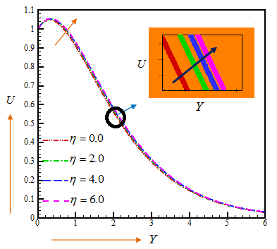
Figure 3. Influence of η on velocity
It is worth mentioning here that Figures. 3-18 are manifested for velocity, microrotation, temperature, concentration, streamlines, isotherms, and iso-concentration to assess the fascinating features of the current problem. Figures. 3-4, in some respects, exhibit the velocity and micro-rotation outlines for various values of η. It can be seen from Figure 3, that the nanofluid velocity increase (see the open circle and the enlarged zone) due to the rise in the value of η.
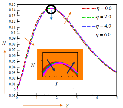
Figure 4. Influence of η on the angular velocity.
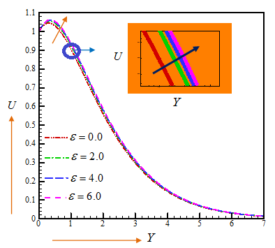
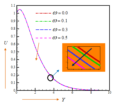
Furthermore, Figure 4 indicates that augmenting values of η depreciates the micro-rotation in the domain 0≤Y≤1.6 and enhances the micro-rotation in the domain 1.6≤Y≤5. For several values of variable electrical conductivity parameter ε, the features of velocity are, in some respects, bestowed in Figure 5. It is pointedly surveyed that, both the fluid velocity ordinations are an elevating feature of ε. Figure 6 signifies the impression of ω on velocity profiles. In point of fact, ω demarcates the contribution of relaxation time to specific process time. Ergo, a more substantial value of ω inflates the relaxation time of the nanofluid which retards the movement of nanoparticles. It is conspicuous from Figure 6 that, as the ω accelerates, the fluid velocity annihilates.
Figure 5. Influence of ε on velocity
Figure 6. Influence of ω on velocity
The aftermaths conceived for ω on velocity field in this dissertation is in an excellent bargain with the evaluated upshots of Nadeem et al. [21], Hayat et al. [22], Malik et al. [23]. Williamson parameter, ω, has a little influence on the nanofluid velocity; however, the velocity tendency has never been changed. And therefore, an arbitrary region (open circle) has been enlarged to identify clearly where the velocity profiles get influenced (decreases with an increase in ω). That blue arrow is indicating the enlarged view of the open circle zone.
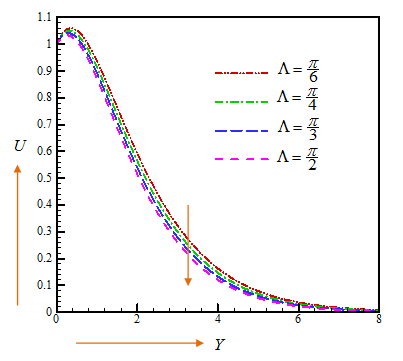
Figure 7. Influence of $\Lambda$ on velocity
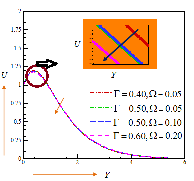
Figure 8. Influence of $\Gamma$ and $\Omega$ on velocity
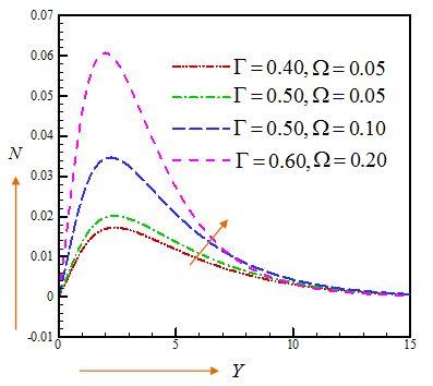
Figure 9. Influence of $\Gamma$ and $\Omega$ on angular velocity
The upshots of Lorentz angle (Λ) on velocity is strategised in Figure 7. From the graphs, it is noticed that the upturning values of Λ deplete the fluid velocity; that is because Lorentz force generates a hindrance to the movements of the fluid velocity. The upshot of inclined angle Λ on the velocity field in our investigation is similar to the examined outcomes of Khan et al. [24]. Figures. 8-9, in some respects, demonstrate the impact of Γ and Ω on the fluid velocity and micro-rotation fields. From Figures. 8-9, It is identified that an escalating of Γ and Ω causes a decrease and an increase in velocity and angular velocity respectively, which is analogous with the recorded consequences of Rup and Nering [16], Nering and Rup [17]. Micropolar Parameter, Γ, has much influence on the velocity field than Micro-inertia parameter, Ω. As it is evident from Figure 8 that, due to the same value of Γ = 0.5, the impact on velocity are insignificant although Ω values were dissimilar. Influence of Γ and Ω on the velocity and angular velocity are different although they both possess similar condition Γ = 0.5, Ω = 0.05 and Γ = 0.5, Ω = 0.10”. This can be attributed because an increment in the micropolar parameter, Γ, causes an increment in the viscosity of the fluid, which results in a significant increment in the angular velocity. Furthermore, increasing Γ leads to rising total coherence of the flow, which thus retards the flow.
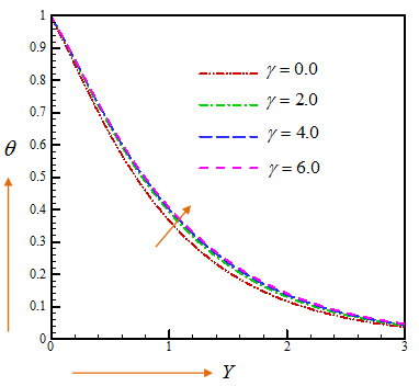
The attributes of parameter γ on fluid temperature profiles portrayed in Figure 10. Additionally, it is patently scrutinised that, larger values of γ aggrandises the fluid temperature. The consequence of thermal conductivity parameter on temperature features in this analysis consents with the upshot unmasked by Rahman et al. [15] and Malik et al. [23].
Figure 10. Influence of γ on temperature layer
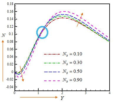
Figure 11. Influence of Nb on angular velocity
Also, it is translucent from Figure 10 that, the temperature features increase with the increment of 0 ≤ γ ≤6. Figure 11 scrutinise the effect of Nb on micro-rotation fields. Accrual in Nb aggravates the promiscuous movement and percussion among the nanoparticles of the fluid which fabricates more heat; ultimately it upshots emaciate in nanoparticle concentration. Furthermore, it can be substantiated from Figure 11 that, the micro-rotation outlines descend in the precinct 0≤Y≤1.2 and ascend in the precinct 1.2≤Y≤4 with a climb in Nb.
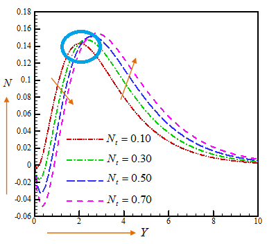
Figure 12. Influence of Nt on angular velocity
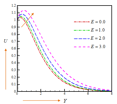
Figure 13. Influence of E on velocity
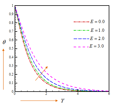
Figure 14. Influence of E on temperature layer
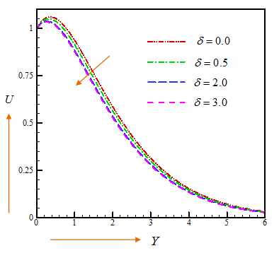
The micro-rotation field for several values of Nt is addressed in Figure 12. It can be sighted that, micro-rotation has an ebbing attitude in the realm 0≤Y≤2 and a thriving outlook in the realm 2≤Y≤10 for flourishing values of Nt. Figures 13-15, convey the characteristics of E on boundary layer flow. It is because of the sooth that more lavish values of E accumulate compressive chemical reaction rate, in this fashion concentration exacerbated. The behaviour of δ on rate and micro-rotation are publicised in Figures. 16-17. Moreover, it is incontestably evinced that, heavier values of temperature relative parameter δ dwindle the fluid velocity outlines. Alongside, we can gaze from Figure 17 that, the increment of δ upturns the micro-rotation in the bailiwick 0≤Y≤1.6 and descends in the bailiwick 1.6≤Y≤6.
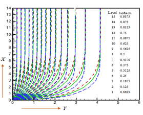
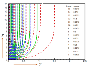
The upshot of Le on streamlines, isotherms, and iso-concentration are captured in Figures. 18a-c. As a matter of fact, Le stipulates the fraction of thermal and mass diffusivity, which is deployed to dilate the fluid drifts. Figure 18a demonstrates the impacts of Le on streamlines; evidently, an increment in Le leads to an ascent in the velocity profile. Furthermore, Lewis number appraises temperature and volume fraction profiles. It is worth noting that, the temperature patterns usurping due to the large number of Le. From the Figure 18c, it is conspicuously spotted that the enhancing rates of Le slacken concentration profiles.
Figure 15. Influence of E on nanoparticle concentration layer
Figure 16. Influence of δ on velocity
(a)
(b)
(c)
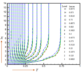
Figure 17. (a) Streamlines, (b) Isotherms and (c) Isoconcentration for Buoyancy ratio parameter λB=0 (Red dashed line), λB=1 (Green solid line) and λB=4 (Blue long-dashed line).
(a)
(b)
(c)
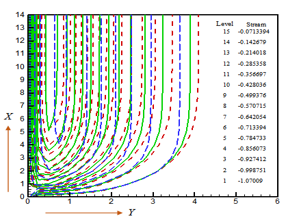
Figure 18. (a) Streamlines, (b) Isotherms and (c) Isoconcentration for Lewis number Le=5 (Red dashed line), Le=10 (Green solid line) and Le=15 (Blue long-dashed line)
The authenticity of the present numerical solution is prevailed by making a comparison with the existing literature and is detected to be an exquisite accent. Conclusively, the principal findings are given below:
i). The velocity is contemplated as an abating function of variable viscosity, inclined Lorentz angle, temperature relative and Williamson parameters while it acts as a developing function for activation energy and variable electrical conductivity parameters.
ii). The angular momentum aggravates for upsurging values of variable viscosity, micropolar and micro-inertia parameters while micropolar and micro-inertia parameter diminishes the velocity fields.
iii). Temperature profiles increase with increasing E and γ, respectively.
iv). Angular velocity profiles first decrease, and after time variation, it increases for Brownian, and thermophoresis parameters.
v). Developing values of buoyancy ratio parameter increases the thickness of momentum boundary layers and diminish the temperature, and nanofluid volume fraction distributions, whereas rising data of Lewis number showed reverse phenomena on the respective fields.
The steady-state explication of our present problem is procured for a non-dimensional time τ≥20.
[1] Choi, S.U.S., Eastman, J. (1995). Enhancing thermal conductivity of fluids with nanoparticles. Proc. ASME Int. Mech. Eng. Cong. Expo., p. 66. https://www.osti.gov/biblio/196525
[2] Khan, M.S., Karim, I., Ali, L.E., Islam, A. (2012). Unsteady MHD free convection boundary-layer flow of a nanofluid along a stretching sheet with thermal radiation and viscous dissipation effects. Int. Nano Lett., 2: 1-9. https://doi.org/10.1186/2228-5326-2-24
[3] Mamun, A.A., Arifuzzaman, S.M., Reza-E-Rabbi, S.K., Biswas, P., Khan, M.S. (2019). Computational modelling on MHD radiative Sisko nanofluids flow through a nonlinearly stretching sheet. International Journal of Heat Technology, 37(1): 285-295. https://doi.org/10.18280/ijht.370134
[4] Hayat, T., Aziz, A., Muhammad, T., Alsaedi, A. (2017). A revised model for Jeffrey nanofluid subject to convective condition and heat generation/absorption. PLoS One, 12(2): e0172518. https://doi.org/10.1371/journal.pone.0172518
[5] Arifuzzaman, S.M., Khan, M.S., Mamun, A.A., Reza-E-Rabbi, S.K., Biswas, P., Karim, I. (2019). Hydrodynamic stability and heat and mass transfer flow analysis of MHD radiative fourth-grade fluid through porous plate with chemical reaction. J. King Saud Univ. Sci., Article in press. https://doi.org/10.1016/j.jksus.2018.12.009
[6] Arifuzzaman, S.M., Khan, M.S., Mehedi, M.F.U., Rana, B.M.J., Ahmmed, S.F. (2018). Chemically reactive and naturally convective high-speed MHD fluid flow through an oscillatory vertical porous-plate with heat and radiation absorption effect. Engineering Science and Technology, an International Journal, 21(2): 215-228. https://doi.org/10.1016/j.jestch.2018.03.004
[7] Reza-E-Rabbi, S.K., Arifuzzaman, S.M., Sarkar, T., Khan, M.S., Ahmmed, S.F. (2018). Explicit finite difference analysis of an unsteady MHD flow of a chemically reacting Casson fluid past a stretching sheet with Brownian motion and thermophoresis effects. Journal of King Saud University – Science, in press. https://doi.org/10.1016/j.jksus.2018.10.017
[8] Arifuzzaman, S.M., Biswas, P., Mehedi, M.F.U., Ahmmed, S.F., Khan, M.S. (2018). Analysis of unsteady boundary layer viscoelastic nanofluid flow through a vertical porous plate with thermal radiation and periodic magnetic field. Journal of Nanofluids, 7(6): 1022-1029. http://dx.doi.org/10.1166/jon.2018.1547
[9] Sarker, T., Arifuzzaman, S.M., Khan, M.S., Reza-E-Rabbi, S.K., Ahmed, R., Ahmmed, S.F. (2018). Unsteady magnetohydrodynamic Casson nanofluid flow through moving cylinder with Brownian and thermophoresis effects. Annales de Chimie - Science des Matériaux, 42(2): 181-207. http://dx.doi.org/10.3166/acsm.42.181-207
[10] Arifuzzaman, S.M., Khan, M.S., Hossain, K.E., Islam, M.S., Akter, S., Roy, R. (2017). Chemically reactive viscoelastic fluid flow in presence of nano particle through porous stretching sheet. Frontiers in Heat and Mass Transfer, 9(5): 1-11. http://dx.doi.org/10.5098/hmt.9.5
[11] Arifuzzaman, S.M., Khan, M.S., Islam, M.S., Islam, M.M., Rana, B.M.J., Biswas, P., Ahmmed, S.F. (2017). MHD Maxwell fluid flow in presence of nano-particle through a vertical porous–plate with heat- generation, radiation absorption and chemical reaction. Frontiers in Heat and Mass Transfer, 9(25): 1-14. http://dx.doi.org/10.5098/hmt.9.25
[12] Khan, M.S., Rahman, M.M., Arifuzzaman, S.M., Biswas, P., Karim, I. (2017). Williamson fluid flow behaviour of MHD convective and radiative Cattaneo-Christov heat flux type over a linearly stretched surface with heat generation, viscous dissipation and thermal-diffusion. Frontiers in Heat and Mass Transfer, 9(15): 1-11. http://dx.doi.org/10.5098/hmt.9.15
[13] Biswas, P., Arifuzzaman, S.M., Rahman, M.M., Khan, M.S. (2018). Effects of periodic magnetic field on 2D transient optically dense grey nanofluid over a vertical plate: A computational EFDM study with SCA. Journal of Nanofluids, 7(1): 1–10. https://doi.org/10.1166/jon.2018.1434
[14] Eringen, A.C. (1966). Theory of micropolar fluids. Journal of Mathematics and Mechanics, 16(1): 1-18. https://doi.org/10.1512/iumj.1967.16.16001
[15] Rahman, M.M., Aziz, A., Lawatia, M.A.A. (2010). Heat transfer in micropolar fluid along an inclined permeable plate with variable fluid properties. International Journal of Thermal Sciences, 49(6): 993-1002. https://doi.org/10.1016/j.ijthermalsci.2010.01.002
[16] Rup, K., Nering, K. (2014). Unsteady natural convection in micropolar nanofluids. Archives of Thermodynamics, 35(3): 155-170. https://doi.org/10.2478/aoter-2014-0027
[17] Nering, K., Rup, K. (2016). The effect of nanoparticles added to heated micropolar fluid. Superlattices and Microstructures, 98: 283-294. https://doi.org/10.1016/j.spmi.2016.08.013
[18] Arifuzzaman, S.M., Mehedi, M.F.U., Mamun, A.A., Biswas, P., Islam, M.R., Khan, M.S. (2018). Magnetohydrodynamic micropolar fluid flow in presence of nanoparticles through porous plate: A numerical study. International Journal of Heat and Technology, 36(3): 936-948. https://doi.org/10.18280/ijht.360321
[19] Arifuzzaman, S.M., Rana, B.M.J., Ahmed, R., Ahmmed, S.F. (2017). Cross diffusion and MHD effect on a high order chemically reactive micropolar fluid of naturally convective heat and mass transfer past through an infinite vertical porous medium with a constant heat sink. AIP Conference Proceedings, 1851: 020006. https://doi.org/10.1063/1.4984635
[20] Williamson, R.V. (1929). The theory of pseudoplastic materials. Ind. Eng. Chem., 21(11): 1108-1111. https://pubs.acs.org/doi/abs/10.1021/ie50239a035
[21] Nadeem, S., Hussain, S.T., Changhoon, L. (2013). Flow of a Williamson fluid over a stretching sheet. Brazilian Journal of Chemical Engineering, 30(3): 619-625. https://doi.org/10.1590/S01046632201300030009
[22] Hayat, T., Shafiq, A., Alsaedi, A. (2016). Hydromagnetic boundary layer flow of Williamson fluid in the presence of thermal radiation and Ohmic dissipation. Alexandria Engineering Journal, 55(3): 2229-2240. https://doi.org/10.1016/j.aej.2016.06.004
[23] Malik, M., Bibi, M., Khan, F., Salahuddin, T. (2016). Numerical solution of Williamson fluid flow past a stretching cylinder and heat transfer with variable thermal conductivity and heat generation/absorption. AIP Adv., 6: 035101. https://doi.org/10.1063/1.4943398
[24] Khan, M., Malik, M.Y., Salahuddin, T., Hussian, A. (2018). Heat and mass transfer of Williamson nanofluid flow yield by an inclined Lorentz force over a nonlinear stretching sheet. Results in Physics, 8: 862-868. https://doi.org/10.1016/j.rinp.2018.01.005
[25] Bestman, A.R. (1990). Natural convection boundary layer with suction and mass transfer in a porous medium. International Journal of Energy Research, 14(4): 389-396. https://doi.org/10.1002/er.4440140403
[26] Arrhenius, S. (1889). Über die dissociationswärme und den einfluss der temperatur auf den dissociationsgrad der elektrolyte. Z. Phys. Chem., 4U(1): 96–116. https://doi.org/10.1515/zpch-1889-0408
[27] Maleque, K.A. (2013). Effects of exothermic/endothermic chemical reactions with Arrhenius activation energy on MHD free convection and mass transfer flow in presence of thermal radiation. Journal of Thermodynamics, 2013: 1-11. http://dx.doi.org/10.1155/2013/692516
[28] Mustafa, M., Khan, J.A., Hayat, T., Alsaedi, A. (2017). Buoyancy effects on the MHD nanofluid flow past a vertical surface with chemical reaction and activation energy. International Journal of Heat and Mass Transfer, 108: 1340-1346. https://doi.org/10.1016/j.ijheatmasstransfer.2017.01.029
[29] Ramzan, M., Ullah, N., Chung, J.D., Lu, D., Farooq, U. (2017). Buoyancy effects on the radiative magneto micropolar nanofluid flow with double stratification, activation energy and binary chemical reaction. Sci. Rep., 7: 1-15. https://doi.org/10.1038/s41598-017-13140-6
[30] Zeeshan, A., Shehzad, N., Ellahi, R. (2018). Analysis of activation energy in Couette-Poiseuille flow of nanofluid in the presence of chemical reaction and convective boundary conditions. Results in Physics, 8: 502-512. https://doi.org/10.1016/j.rinp.2017.12.024
[31] Atif, S.M., Hussain, S., Sagheer, M. (2018). Numerical study of MHD micropolar Carreau nanofluid in the presence of induced magnetic field. AIP Advances, 8(3): 01-20. https://doi.org/10.1063/1.5022681
[32] Muthtamilselvan, M., Ramya, E., Doh, D.H., Cho, G. (2018). Heat transfer analysis of a Williamson micropolar nanofluid with different flow controls. Journal of Mechanics, 1-14. https://doi.org/10.1017/jmech.2018.37