OPEN ACCESS
Debris flow is a multi-phase liquid flow with high bulk density and complex components. The velocity of a debris flow is one key part of debris flow dynamics, which is essential to know in order to formulate a plan for early hazard warnings and mitigation. The normal methods of calculating debris flow velocity have their limits due to the difficulty in precisely determining parameters, resulting in unsatisfactory predictions. In this article, we propose a new hybrid prediction model to estimate the debris flow velocity, which is based on the empirical equation of flow velocity calculation combined with a least squares support vector machine (LSSVM) and Particle swarm optimization (PSO). The new method can improve the performance of velocity empirical equations. The result has shown that the new hybrid model is better than the former method and it exhibits high potential for becoming a useful tool for identifying debris flow velocity.
Debris Flow, Empirical Equations, Velocity Calculation, LSSVM, PSO
Debris flow is a mass liquid-like movement involving water-saturated, predominantly coarse-grained material which is moving down a confined and steep channel at a high speed [1]. It poses a threat to human life and can cause enormous property damages involving both direct and indirect costs. Debris flows of various sizes, depths, and velocities often endanger human lives and infrastructure facilities, and can result in fatalities [2]. The velocity of a debris flow is associated with run-out distance, superelevation, impact force, and influences hazard assessment [3]. Therefore, it is a very important factor in hazard evaluation and mitigation[4]. Many scholars have done a large amount of work to estimate debris flow velocity, including empirical equation based on the Manning formula, numerical simulation, and Machine Learning theory as widely applied to debris flow velocity analysis.
The velocity calculation methods of debris flow can be categorized into four types [5]. The first is numerical simulation equations [6]. This calculation method is based on the continuum theory, mass and momentum conservation equations, and the velocity formula is derived from basic physical principles. Most parameters of the velocity equation are obtained from laboratory experiments, and some are difficult to obtain and can only be back-analyzed through field survey, which limits its application. The second method is empirical equations, where most equations are derived from the Manning-Stickler equation or the Chezy equation, and is summarized from experimental observations [7]. The third method is back-calculated from super elevation events. The super elevation height is related to the flow surface at the outside and inside walls, which can back-calculate the debris flow velocity. However, this method requires subjective estimates of radii of curvature of bends in the debris flow channel, and the result may change according to various person’s estimations [8]. The fourth method is based on data statistics or the machine learning method, which require a large amount of data, and the result of this method is predicated on velocity influence factors through machine learning theory.
The support vector machine (SVM), developed by Vapnik and his colleagues, is based on the structural risk minimization principle and statistic learning theory (SLT) [9]. Different from other machine learning methods, SVM do not use all available samples and has a smaller structural risk, so it can solve the problem with small samples and achieve a good generalization capability [10]. It is well suited to engineering geological prediction problems and shows good performance in nonlinear high-dimensional prediction [11]. However, having appropriate parameters for the SVM model is crucial to ensure the best performance. Therefore, the optimal method for determining SVM parameters is essential, and the particle search optimal (PSO) algorithm is introduced for the best performance of the SVM model [12].
This study focuses on mean debris flow velocity. Through the analysis of empirical velocity calculation equations, the parameters for debris flow velocity calculation are determined, and the LSSVM and PSO methods are introduced to predict the parameters of the common empirical equation. The empirical equation is combined with machine learning theory to calculate the debris flow velocity, and the result shows a better performance than the original empirical equation, as summarized in the conclusion.
2.1 Empirical equation of debris flow velocity
The empirical or semi-empirical formula for the calculation of average flow velocity have been proposed by many researchers. The factors that account for the largest differences of each equation are related to the properties of debris flow materials, the slope of the flow channel and the depth of the debris flow, all of which are used in every equation. The most well known equations for debris flow velocity calculation are as follows:
1) The Manning formula
$V=\frac{1}{n}{{R}^{2/3}}{{S}^{1/2}}$ (1)
where n is the resistance coefficient, R is the hydraulic radius, and S is the slope.
2) Newtonian laminar flow
$V=\frac{1}{3}\frac{\rho g{{h}^{2}}S}{\mu }$ (2)
where $\rho $ is debris flow density, g is gravitational acceleration, h is debris flow depth, $\mu $ is dynamic viscosity.
3) Bingham fluid
$V=\frac{\rho g{{H}^{2}}S}{2\eta }\left( 1-\frac{H}{3h} \right)$ (3)
where, H is effective shear depth, $\eta $ is Bingham viscosity.
A widely-used method for mean velocity is the Manning-stickler equation, and all aforementioned formulas are based on it. The Manning coefficient n is adjusted through statistical regression analysis based on observation data, and the empirical formula of the research area is obtained. In calculating the velocity of a debris flow, the Manning coefficient n is subjectively determined, but it is closely associated with the accuracy of the results. Generally, the common equations of flow mean velocity calculation can be described as follows:
$V=N{{h}^{b}}{{S}^{c}}$ (4)
where b, c and N are constant values, They can be determined by the research data from the debris flow area.
In this article, debris flow velocity is calculated by the common equation of flow, and the parameters used in the mean flow equation is the integral component in debris flow velocity calculation.
2.2 LS-SVM prediction principle
The least squares support vector machine was developed by Suykens et al. [13]. It is one of the most accessible data mining technologies for small samples based on the structural risk minimization principle. The non-linear prediction problem is resolved by conducting original data into high dimensional space and obtaining the optimal hyperplane. The dimension transformation is conducted by kernel function, so the kernel function is important for prediction accuracy. RBF kernel is selected in this article, and is expressed as follows:
$K({{x}_{i}},{{x}_{j}})=\exp (-\gamma {{({{x}_{i}}-{{x}_{j}})}^{2}})$ (5)
The prediction function of a common fitness curve can be describe as $\ y(x)={{w}^{T}}\varphi (x)+{{w}_{0}}$, where $w$ is the weight vector, ${{w}_{0}}$ is the bias term, $\gamma $ is a constant which should be determined artificially, It is closely associated with the performance of the LSSVM model, and PSO is applied for it's optimization. The structural risk minimization is used to resolve the problem, and it formulates the following optimization problem:
$\left\{ \begin{align} & \min \ \ J(w,\xi )=\frac{1}{2}{{\left\| w \right\|}^{2}}+C\sum\limits_{i=1}^{l}{\xi _{i}^{2}} \\ & s.t.\ \ \ {{y}_{i}}={{w}^{T}}\varphi ({{x}_{i}})+{{w}_{0}}+{{\xi }_{i}},\ \ i=1,2\cdot \cdot \cdot l \\\end{align} \right.$ (6)
where $K({{x}_{i}},{{x}_{j}})=\varphi ({{x}_{j}})\cdot \varphi ({{x}_{i}});{{R}^{n}}\to {{R}^{{{n}_{h}}}}$ is the kernel function, $w\in {{R}^{{{n}_{h}}}}$ is a weight vector, C is the penalty parameter, ${{\xi }_{i}}\in R$ is an error variant, ${{w}_{0}}$ is a deviation.
To solve the function, we introduce the Lagrannge multiplier, than the function can be defined as follows:
$L(w,{{w}_{0}},\xi ,\alpha )=\frac{1}{2}{{w}^{T}}\cdot w+C\sum\limits_{i=1}^{l}{\xi _{i}^{2}}-\sum\limits_{i=1}^{l}{{{\alpha }_{i}}}({{w}^{T}}\cdot \varphi ({{x}_{i}})+{{w}_{0}}+{{\xi }_{i}}-{{y}_{i}})$ (7)
${{\alpha }_{i}},i=1,2....l$ is the Lagrange multiplier, set $\frac{\partial L}{\partial w},\frac{\partial L}{\partial {{w}_{0}}},\frac{\partial L}{\partial \alpha },\frac{\partial L}{\partial \xi }$ to zero, $\min \ \ J(w,\xi )$ will be optimized. Then we get:
$\left[ \begin{matrix} 0 & 1 & \cdots & 1 \\ 1 & K({{x}_{1}},{{x}_{1}})+1/C & \cdots & K({{x}_{1}},{{x}_{l}}) \\ \vdots & \vdots & \ddots & \vdots \\ 1 & K({{x}_{l}},{{x}_{1}}) & \ldots & K({{x}_{l}},{{x}_{l}})+1/C \\\end{matrix} \right]\left[ \begin{matrix} b \\ {{\alpha }_{1}} \\ \vdots \\ {{\alpha }_{l}} \\\end{matrix} \right]=\left[ \begin{matrix} 0 \\ {{y}_{1}} \\ \vdots \\ {{y}_{l}} \\\end{matrix} \right]$ (8)
We calculate ${{w}_{0}}$, by (6) (7) (8),Then the prediction model function is as follows:
$f\left( x \right)=\sum\limits_{i=1}^{l}{{{\alpha }_{i}}}K({{x}_{i}},x)+{{w}_{0}}$ (9)
2.3 PSO (particle swarm optimization) method
PSO (particle swarm optimization) is an optimization method for SVM parameters used in this article, which is an improved method of the grid search method. It sets each possible solution as a particle in the optimization process, and gives it an initial speed so that the particle can move in high dimension space. The best choice of one particle and all particles in optimization are recorded as the individual optimal solution ${{p}_{best}}$ and the global optimal solution ${{g}_{best}}$, and the speed changes with ${{p}_{best}}$ and ${{g}_{best}}$ in high dimension space are recorded. After several loops of particles’ changing speeds and positions, the finally optimal solution of parameters are obtained [14].
$+{{c}_{2}}\cdot rand()\times ({{g}_{best}}-{{x}_{i}}(t))$ (10)
${{x}_{i}}(t+1)={{x}_{i}}(t)+{{v}_{i}}(t+1)$ (11)
where ${{v}_{i}}$ is the velocity of the i particle, ${{x}_{i}}$ is the position of the particle, ${{c}_{1}}$ and ${{c}_{2}}$ are learning factors, $\omega $is the inertia factor.
2.4 Improved empirical equation of velocity calculation
According to studies worldwide, the general equation of flow velocity based on the Manning formula is as equation: $V=N{{h}^{b}}{{S}^{c}}$ , where N is a constant, h is flow depth, b and c are coefficients with regional features. Previous studies have yielded the following results. In the Chezy equation, b=c=0.5. In the Manning-Strickler equation, b is 2/3 and c is 1/2. In the debris flow velocity research articles, the b value is varied from 1/3 to 1/2, with 1/2 as the most widely used for debris flow velocity calculation. c is varied from 1/6 to 1, and the c value is generally determined as 1/2 or 1/3 [5].
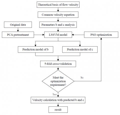
The values of b and c in the equations are influenced by many factors of debris flow materials. In this article, we propose a PSO-LSSVM model to analysis the coefficients in the empirical equation, and the process of velocity calculation is as follows.
1) The original data of debris flow samples are processed by PCA.
2) The b value is fixed as 0.5, and the c values of each samples are back-calculated through empirical formula.
3) Train the LSSVM model with debris flow samples and the back-calculated c value.
4) Calculate MSE and MAE through five-fold cross-
validation, and obtain the predicted c value based on the LSSVM model.
5) Fix c value as 1, then calculate b as the same as procedures 3) and 4) instead of c parameter.
6) Put the new predicted b and c vectors into the empirical formula, the velocity of debris flow samples will be obtained through the new equation.
3.1 Debris flow data and background
The debris flow data used for SVM velocity prediction in this study is from Jiangjia Ravine, located in Yunnan province in China. The ravine is 12.1 km long with a total area of 47.1 km2. The altitude is from 1088m to 3269m above sea level, and several debris flows occur each year in this section. According to previous articles, ρ, h, S, p, D50, D50/D10, and h/D50 are potential factors influencing debris flow velocity. The Manning formula and other articles [8,15,16,17] have shown that the most important influencing factors in debris flow velocity are channel characteristics and material properties, such as slope gradient , wetted perimeter and roughness, flow depth related to wetted perimeter in shallow and wide debris flow gullies, particle mean diameter and density reflecting roughness. We take the particle mean diameter, flow depth, slope gradient and density as the influencing factors in debris flow velocity prediction. We select 50 samples of debris flow gullies in Jiangjia Ravine for debris flow velocity prediction, with test data taken from article [18].
The 50 debris flow gullies in the research area are shown in Table 1. Figure 1 shows the procedure of the improved empirical velocity model in this paper.
Table 1. Debris flow samples for velocity prediction of research area
|
Particle mean diameter (mm) |
Flow depth (m) |
Slope gradient (%) |
Densit (t/m3) |
Velocit (m/s) |
Particle mean diameter (mm) |
Flow depth (m) |
Slope gradient (%) |
Density (t/m3) |
Velocity (m/s) |
||
|
1 |
8 |
1.75 |
6.3 |
2.08 |
8.9 |
26 |
9 |
2.5 |
5.5 |
2.22 |
6.9 |
|
2 |
11 |
1.5 |
6.3 |
2.2 |
8.8 |
27 |
11 |
2.26 |
5.5 |
2.13 |
6.6 |
|
3 |
17 |
2 |
6.3 |
2.21 |
7.4 |
28 |
8 |
1.2 |
5.5 |
2.2 |
6 |
|
4 |
14 |
2 |
6.3 |
2.25 |
7.9 |
29 |
11 |
1.45 |
5.5 |
2.25 |
7.4 |
|
5 |
6 |
0.95 |
6.3 |
2.16 |
10 |
30 |
11 |
0.65 |
5.5 |
2.24 |
5 |
|
6 |
9 |
0.55 |
6.3 |
2.25 |
7.4 |
31 |
10 |
1.22 |
5.5 |
2.21 |
6.9 |
|
7 |
7 |
0.11 |
6.3 |
2.07 |
7.6 |
32 |
16 |
1.68 |
5.5 |
2.28 |
7.5 |
|
8 |
9 |
1 |
6.3 |
2.19 |
7.6 |
33 |
12 |
3.72 |
6.6 |
2.21 |
9.2 |
|
9 |
10 |
0.9 |
6.3 |
2.21 |
7.3 |
34 |
12 |
1.07 |
5.5 |
2.29 |
5.8 |
|
10 |
12 |
0.7 |
6.3 |
2.19 |
6.6 |
35 |
1 |
0.52 |
5.8 |
1.7 |
3.6 |
|
11 |
16 |
2.75 |
6.6 |
2.21 |
9.6 |
36 |
8 |
1.03 |
5.5 |
2.21 |
5.8 |
|
12 |
11 |
1.7 |
6.6 |
2.19 |
7.5 |
37 |
3 |
0.7 |
5.5 |
1.92 |
5.6 |
|
13 |
8 |
2.1 |
6.6 |
2.2 |
8.4 |
38 |
2 |
0.7 |
5.8 |
1.8 |
4.1 |
|
14 |
12 |
1.6 |
6.6 |
2.22 |
8.1 |
39 |
3 |
0.93 |
5.8 |
1.92 |
4.8 |
|
15 |
7 |
1.3 |
6.6 |
2.2 |
8.2 |
40 |
2 |
0.56 |
5.8 |
1.69 |
3.6 |
|
16 |
15 |
2.2 |
6.6 |
2.29 |
9.6 |
41 |
2 |
0.5 |
5.8 |
1.76 |
3.5 |
|
17 |
12 |
2.1 |
6.6 |
2.21 |
9.4 |
42 |
6 |
0.6 |
5.5 |
1.99 |
4.9 |
|
18 |
10 |
2.1 |
6.3 |
2.29 |
9.3 |
43 |
5 |
0.6 |
5.5 |
1.97 |
4.7 |
|
19 |
15 |
2 |
6.3 |
2.3 |
8.5 |
44 |
10 |
1.61 |
5.5 |
2.25 |
7.7 |
|
20 |
3 |
0.4 |
6.3 |
2.04 |
4 |
45 |
11 |
1.77 |
5.5 |
2.24 |
7.7 |
|
21 |
6 |
1.4 |
6.3 |
1.95 |
7.8 |
46 |
1 |
0.6 |
5.5 |
1.83 |
3.9 |
|
22 |
1 |
0.4 |
6.3 |
2.02 |
3.7 |
47 |
8 |
0.55 |
5.8 |
2.07 |
3.9 |
|
23 |
1 |
0.4 |
6.3 |
1.85 |
3.8 |
48 |
11 |
1.09 |
5.5 |
2.25 |
6.4 |
|
24 |
11 |
2.1 |
6.3 |
2.21 |
9.3 |
49 |
1 |
0.55 |
5.8 |
1.8 |
3.7 |
|
25 |
17 |
2.02 |
5.5 |
2.27 |
6.9 |
50 |
6 |
1.25 |
6.3 |
2.1 |
7.6 |
Figure 1. Flowchart of the improved empirical velocity model
3.2 Techniques compared and prediction results
The LSSVM model based on the performance of the empirical equation is sensitive to the b and c values in the empirical equation. In this article, N is determined as 1. The mean MSE with a five-fold cross-validation is used to assess the performance of the SVM prediction model, $MSE=\frac{1}{n}\sum\limits_{i=1}^{n}{{{(f({{x}_{i}})-{{y}_{i}})}^{2}}}$.
The 50 debris flow prediction samples and parameter b, c and its relative velocity results are shown in Table 2. The parameters b and c are predicted by PSO-LSSVM. The origin is the velocity of the field survey. ESb and ESc are the predicted values of b and c through PSO-LSSVM. The bv is the calculated velocity with ESb determined through the general equation of flow velocity ($V=N{{h}^{b}}{{S}^{c}}$). At this time, c is fixed as 1. The cv is the calculated velocity with ESc, and b is fixed as 0.5. The cv is better than bv according to the MSE and MAE.
Table 2. Debris flow velocity estimating with predicted b or c parameter by the empirical equation
|
NO. |
Origin |
ESb |
bv |
ESc |
cv |
NO. |
Origin |
ESb |
bv |
ESc |
cv |
|
1 |
8.9 |
-0.19 |
5.67 |
1.17 |
11.36 |
27 |
6.6 |
0.59 |
8.89 |
1.00 |
8.34 |
|
2 |
8.8 |
0.18 |
6.79 |
1.06 |
8.58 |
28 |
6 |
0.59 |
6.12 |
1.02 |
6.21 |
|
3 |
7.4 |
0.39 |
8.26 |
0.95 |
8.11 |
29 |
7.4 |
0.58 |
6.82 |
1.01 |
6.71 |
|
4 |
7.9 |
0.38 |
8.21 |
0.96 |
8.35 |
30 |
5 |
0.60 |
4.25 |
1.02 |
4.57 |
|
5 |
10 |
-0.22 |
6.37 |
1.20 |
8.81 |
31 |
6.9 |
0.60 |
6.20 |
1.01 |
6.22 |
|
6 |
7.4 |
-0.05 |
6.49 |
1.13 |
5.93 |
32 |
7.5 |
0.45 |
6.95 |
0.98 |
6.95 |
|
7 |
7.6 |
-0.07 |
7.33 |
1.19 |
2.96 |
33 |
9.2 |
0.39 |
11.07 |
0.93 |
11.11 |
|
8 |
7.6 |
-0.08 |
6.30 |
1.14 |
8.09 |
34 |
5.8 |
0.56 |
5.71 |
1.01 |
5.76 |
|
9 |
7.3 |
0.02 |
6.29 |
1.11 |
7.31 |
35 |
3.6 |
0.54 |
4.08 |
0.91 |
3.60 |
|
10 |
6.6 |
0.10 |
6.08 |
1.09 |
6.19 |
36 |
5.8 |
0.59 |
5.60 |
1.02 |
5.77 |
|
11 |
9.6 |
0.39 |
9.80 |
0.93 |
9.61 |
37 |
5.6 |
0.45 |
4.69 |
1.03 |
4.88 |
|
12 |
7.5 |
0.35 |
7.93 |
0.97 |
8.08 |
38 |
4.1 |
0.62 |
4.66 |
0.92 |
4.19 |
|
13 |
8.4 |
0.31 |
8.32 |
0.98 |
9.26 |
39 |
4.8 |
0.61 |
5.55 |
0.96 |
5.23 |
|
14 |
8.1 |
0.37 |
7.86 |
0.95 |
7.64 |
40 |
3.6 |
0.56 |
4.20 |
0.91 |
3.72 |
|
15 |
8.2 |
0.21 |
6.97 |
1.03 |
7.93 |
41 |
3.5 |
0.59 |
3.85 |
0.91 |
3.51 |
|
16 |
9.6 |
0.39 |
8.99 |
0.93 |
8.59 |
42 |
4.9 |
0.44 |
4.40 |
1.05 |
4.66 |
|
17 |
9.4 |
0.39 |
8.79 |
0.94 |
8.59 |
43 |
4.7 |
0.43 |
4.41 |
1.05 |
4.65 |
|
18 |
9.3 |
0.33 |
8.02 |
1.00 |
9.18 |
44 |
7.7 |
0.59 |
7.27 |
1.01 |
7.07 |
|
19 |
8.5 |
0.39 |
8.26 |
0.95 |
8.09 |
45 |
7.7 |
0.57 |
7.61 |
1.00 |
7.37 |
|
20 |
4 |
0.26 |
4.96 |
1.09 |
4.71 |
46 |
3.9 |
0.47 |
4.33 |
0.99 |
4.16 |
|
21 |
7.8 |
0.00 |
6.31 |
1.17 |
10.18 |
47 |
3.9 |
0.44 |
4.46 |
1.01 |
4.41 |
|
22 |
3.7 |
0.39 |
4.41 |
1.02 |
4.13 |
48 |
6.4 |
0.59 |
5.79 |
1.01 |
5.86 |
|
23 |
3.8 |
0.44 |
4.20 |
0.95 |
3.64 |
49 |
3.7 |
0.59 |
4.07 |
0.91 |
3.68 |
|
24 |
9.3 |
0.28 |
7.78 |
1.02 |
9.48 |
50 |
7.6 |
-0.21 |
6.01 |
1.20 |
10.15 |
|
25 |
6.9 |
0.43 |
7.43 |
0.98 |
7.54 |
MSE |
|
1.284 |
|
1.305 |
|
|
26 |
6.9 |
0.58 |
9.34 |
1.00 |
8.72 |
MAE |
|
0.827 |
|
0.740 |
|
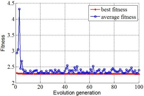
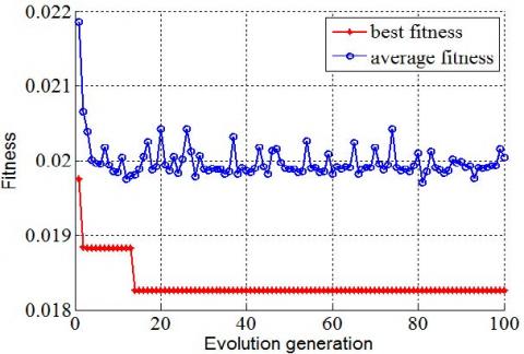
In comparison, b is predicted and c is fixed as a constant, or c is predicted and b is fixed as a constant. Table 3 shows the final result of debris flow velocity calculation based on ESb and ESc. Both ESb and ESc are substituted into the general equation of flow velocity, and the final result of debris flow velocity is calculated by the improved velocity equation. Table 3 shows the result of velocity bcv calculation based on ESb and ESc, with the MSE and MAE being smaller than the other methods shown in Table 2. This table provides the best evidence showing that the improved empirical model has the capability to predict debris flow velocity more efficiently and accurately than only b or c can predict. Figure 2 and Figure 3 show the fitness curve of the PSO process, with lower fitness numbers indicating better performance. ![]() and C of LSSVM are the objective values of PSO. With the increasing of the number of evolution generation, the fitness decreases to a low value and becomes stable. Then the PSO process achieves the best result, and the LSSVM model can result in the most suitable fit. Figure 2 is the fitness curve of b optimization, and Figure 3 is the fitness curve of c optimization.
and C of LSSVM are the objective values of PSO. With the increasing of the number of evolution generation, the fitness decreases to a low value and becomes stable. Then the PSO process achieves the best result, and the LSSVM model can result in the most suitable fit. Figure 2 is the fitness curve of b optimization, and Figure 3 is the fitness curve of c optimization.
Table 3. Debris flow velocity calculation based on both predicted b and c
|
ID |
1 |
2 |
3 |
4 |
5 |
6 |
7 |
8 |
9 |
10 |
|
bcv |
7.74 |
7.55 |
7.52 |
7.70 |
9.14 |
8.23 |
10.37 |
8.09 |
7.69 |
7.14 |
|
ID |
11 |
12 |
13 |
14 |
15 |
16 |
17 |
18 |
19 |
20 |
|
bcv |
8.60 |
7.45 |
8.06 |
7.19 |
7.35 |
7.88 |
7.89 |
8.06 |
7.50 |
5.86 |
|
ID |
21 |
22 |
23 |
24 |
25 |
26 |
27 |
28 |
29 |
30 |
|
bcv |
8.61 |
4.56 |
3.83 |
8.08 |
7.16 |
9.37 |
8.97 |
6.31 |
6.91 |
4.37 |
|
ID |
31 |
32 |
33 |
34 |
35 |
36 |
37 |
38 |
39 |
40 |
|
bcv |
6.35 |
6.77 |
9.66 |
5.78 |
3.51 |
5.78 |
4.97 |
4.02 |
5.19 |
3.59 |
|
ID |
41 |
42 |
43 |
44 |
45 |
46 |
47 |
48 |
49 |
50 |
|
bcv |
3.30 |
4.81 |
4.82 |
7.37 |
7.67 |
4.23 |
4.57 |
5.90 |
3.48 |
8.66 |
|
|
MSE |
0.9753 |
MAE |
0.7272 |
|
|
|
|
||
Figure 2. Fitness curves of optimization of b through PSO
Figure 3. Fitness curves of optimization of c through PSO
1) This article proposed an improved empirical debris flow velocity prediction model and has been shown to predict the debris flow velocity well. The testing sample has shown that the improved new method for debris flow velocity performs better with less MSE and MAE than other methods.
2) The common velocity calculation equation is summarized from several debris flow velocity empirical equations and the Manning-Stickler equation. Some parameters of the equation are associated with debris flow properties and it is predicted by LSSVM, which shows to be a feasible method to determine the parameters of the velocity equation.
3) The number of influencing factors in debris flow velocity is too numerous. According to the analytical and empirical algorithm, the main factors of debris flow velocity are slope gradient S, particle mean diameter D50, flow depth h and density. The parameters b and c are related these factors, but the relation formula is still unclear.
4) The parameters b and c are predicted by LSSVM respectively, and the velocity is calculated with the predicted value. When b is predicted by LSSVM, c is selected as the common value 1; otherwise, b is 0.5. The two methods both have a good performance for debris flow velocity prediction.
5) The predicted values of b and c are lastly substituted into the formula together for the velocity calculation, and the MSE and MAE are the best compared with the other methods, which shows the validity of the improved method.
[1] Iverson R.M. (1997). The physics of debris flows, Reviews of Geophysics, Vol. 35, No. 3, pp. 245–296. DOI: 10.1029/97RG00426
[2] Dowling C.A., Santi P.M. (2014). Debris flows and their toll on human life: a global analysis of debris-flow fatalities from 1950 to 2011, Natural Hazards, Vol. 71, No. 1, pp. 203–227. DOI: 10.1007/s11069-013-0907-4
[3] Tie Y. (2013). Prediction of the run-out distance of the debris flow based on the velocity attenuation coefficient, Natural Hazards, Vol. 65, No. 3, pp. 1589–1601. DOI: 10.1007/s11069-012-0430-z
[4] Rickenmann, D. (1999). Empirical relationships for debris flows, Natural Hazards Vol. 19, No. 1, pp. 47–77. DOI: 10.1023/A:1008064220727
[5] Yang H., Wei F., Hu K. (2014). Mean velocity estimation of viscous debris flows, Journal of Earth Science, Vol. 25, No. 4, pp. 771-778. DOI: 10.1007/s12583-014-0465-z
[6] Armanini A., Fraccarollo L., Rosatti G. (2009). Two-dimensional simulation of debris flows in erodible channels, Computers & Geosciences, Vol. 35, No. 5, pp. 993-1006. DOI: 10.1016/j.cageo.2007.11.008
[7] Venutelli M. (2005). A constitutive explanation of manning’s formula, Meccanica, Vol. 40, No. 3, pp. 281–289. DOI: 10.1007/s11012-005-6529-5
[8] Prochaska A.B., Santi P.M., Higgins J.D., Cannon S.H. (2008). A study of methods to estimate debris flow velocity, Landslides, Vol. 5, No. 4, pp. 431–444. DOI: 10.1007/s10346-008-0137-0
[9] Cortes C., Vapnik V. (1995). Support-vector networks, Machine Learning, Vol. 20, No. 3, pp. 273–297. DOI: 10.1023/A:1022627411411
[10] Khan M.S., Coulibaly P. (2006). Application of support vector machine in lake water level prediction, Journal of Hydrologic Engineering, Vol. 20, No. 11, pp. 199–205. DOI: 10.1061/(ASCE)1084-0699(2006)11:3(199)
[11] Zhu C.H., Hu G.D. (2012). Time series prediction of landslide displacement using SVM model: application to Baishuihe landslide in Three Gorges reservoir area, China, Applied Mechanics & Materials Vol. 239, pp. 1413–1420. DOI: 10.4028/www.scientific.net/AMM.239-240.1413
[12] Wu C.H., Tzeng G.H., Goo Y.J., Fand W.C. (2007). A real-valued genetic algorithm to optimize the parameters of support vector machine for predicting bankruptcy, Expert Systems with Applications, Vol. 32, No. 2, pp. 397–408. DOI: 10.1016/j.eswa.2005.12.008
[13] Shabri A., Suhartono (2012). Streamflow forecasting using leastsquares support vector machines, Hydrological Sciences Journal, Vol. 57, No. 7, pp. 1275-1293. DOI: 10.1080/02626667.2012.714468
[14] Jin C., Jin S., Qin L. (2012). Attribute selection method based on a hybrid BPNN and PSO algorithms, Applied Soft Computing, Vol. 12, No. 8, pp. 2147-2155. DOI: 10.1016/j.asoc.2012.03.015
[15] Lo D.O.K. (2000). Review of natural terrain landslide debris-resisting barrier design. Geotechnical Engineering Office, Civil Engineering Department, The Government of Hong Kong Special Administrative Region, Hong Kong, China, GEO Report No. 104.
[16] Shi M.Y., Chen J.P., Sun D.Y., Cao C. (2015). Hazard assessment of debris flows based on the catastrophe progression method: a case study from the Wudongde Dam site, International Journal of Heat and Technology, Vol. 33, No. 4, pp. 217-220. DOI: 10.18280/ijht.330429
[17] Zhang S.X., Zhang L.T., Qi Q., Li Q., Shi P. (2015). Numerical simulation of the characteristics of debris flow from a tailing pond dam break, International Journal of Heat and Technology, Vol. 33, No. 3, pp. 127-132. DOI: 10.18280/ijht.330319
[18] Xu L., Wang Q., Chen J., et al. (2013). Forecast for average velocity of debris flow based on BP neural network, Journal of Jilin University (Earth Science Edition), Vol. 43, No. 1, pp. 186-191.