Restu Arisanti*![]() | Resa Septiani Pontoh
| Resa Septiani Pontoh![]() | Sri Winarni
| Sri Winarni![]() | Suhaila Prima Putri
| Suhaila Prima Putri![]() | Carissa Egytia Widiantoro
| Carissa Egytia Widiantoro![]() | Silvi
| Silvi![]()
© 2025 The authors. This article is published by IIETA and is licensed under the CC BY 4.0 license (http://creativecommons.org/licenses/by/4.0/).
OPEN ACCESS
Population growth and technological development are fueling the increasing demand for electricity in Indonesia. By 2023, electricity consumption in Indonesia has reached 1,285 KWH, mostly met by non-renewable energy. This condition raises concerns about the sustainability of energy supply. On the other hand, Indonesia has great potential to utilize ocean wave energy as a source of electricity. The novelty of this research lies in the Generalized Linear Model-based Gamma Regression modelling approach to evaluate the electrical energy potential of ocean wave energy in 175 Indonesian waters. The focus of this research lies on the specific analysis of the impact of wave type on power potential, while wind speed and weather factors have no significant influence. In addition, the selection of the best model was conducted using the Root Mean Square Error (RMSE) approach, which shows that the model predictions are getting closer to the actual values. The results show that low and medium wave types significantly reduce the power potential compared to calm waves, by 0.0000083% and 0.0000113%, respectively. These findings make an important contribution to understanding the potential of ocean wave energy as a renewable energy source in Indonesia.
ocean wave, MLE, OWC, MWPP, gamma regression
Energy is a fundamental necessity that supports a wide range of human activities across the globe. As the population grows and economic activities become more complex in the modern era, the demand for energy continues to rise steadily [1]. Population growth and national economic development are key drivers of rising energy consumption in Indonesia [2]. Most homes and facilities used daily require electrical equipment.
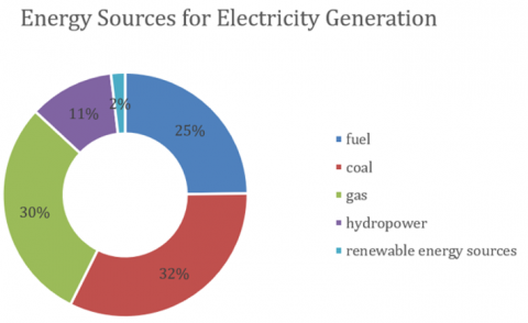
As a result, electricity use in Indonesia is increasing in line with population growth and advances in information and technology. Figure 1 is a pie chart of the wave type variable. Data from the Ministry of Energy and Mineral Resources (ESDM) shows that electricity consumption in 2023 rose to 1,337 kWh per capita, marking a 13.s98% increase from 2022’s figure of 1,173 kWh per capita [3]. Energy sources for electricity generation consists of new renewable energy sources 1.8% (Ministry of Energy and Mineral Resources).
Indonesia’s energy consumption remains heavily reliant on non-renewable sources, particularly fossil fuels, which still surpass renewable energy usage [4, 5]. This is a severe concern for the sustainability of energy supply in the future.
The ocean is renewable energy source, and innovations in current ocean [6-8] energy technology offer the potential to reduce carbon dioxide emissions from electricity generation. This makes it a viable option for long-term, sustainable energy solutions [6, 9].
Indonesia, an archipelago nation with over 17,000 islands and about 65% ocean coverage, has more ocean than land. This provides a substantial opportunity to harness wave energy as tidal energy [10].
A notable advantage of Indonesia's unique geographical characteristics is its extensive coastline of approximately 81,000 km, consistent wave height patterns, and locations with gently sloping seabed topographies, which make it an ideal case for Oscillating Water Column (OWC) technology. A key strength of the region lies in the untapped wave energy potential, which could be efficiently extracted in areas such as East Nusa Tenggara, Central Sulawesi, and other coastal zones, using advanced technologies like OWC. It is now well established that Indonesia's position within the Pacific Ring of Fire and monsoonal wind patterns contributes to a predictable and renewable source of ocean wave energy, offering a sustainable energy solution.
The abundance of ocean area underscores the critical role of wind-driven wave data, which is essential for supporting maritime operations such as determining shipping routes, forecasting ocean hazards, and conducting scientific studies on ocean mixing and air-sea interactions. Additionally, wave energy from Indonesia’s oceans holds promising potential as a renewable energy source for the nation [11].
In economic perspective, the utilization of OWC technology can reduce dependence on fossil fuels, decrease carbon emissions, and provide cost-effective solutions for energy generation in remote and underdeveloped regions, where grid connectivity is limited but wave energy is abundant.
Ocean energy in Indonesia is seen as a promising form of renewable energy [6, 12-15] with the potential to significantly contribute to the global energy mix [6, 16].
Currently, various technologies have been developed for ocean wave power plants, including buoy systems, overtopping devices, and OWC technology [10, 17-22]. OWC technology is well-suited for coastal areas with gently sloping seabed topography and consistent wave height [23]. The suitability of OWC technology for Indonesian waters has been proven through studies in areas such as East Nusa Tenggara, Central Sulawesi, Pantai Baron in Yogyakarta, and Binongko Island in Wakatobi, Southeast Sulawesi. These studies show that OWC technology can efficiently harness wave energy in a variety of environmental conditions.
Previous research conducted in regions such as East Nusa Tenggara [23], Central Sulawesi, Pantai Baron, Gunung Kidul DI Yogyakarya [24], and Binongko Island, Wakatobi, Southeast Sulawesi [25], the OWC technology has been utilized to analyze ocean wave energy potential, leading us to select this technology for analyzing Indonesian waters.
There is a growing body of literature that recognizes the importance of identifying the specific factors influencing the potential power of ocean waves in Indonesia. However, a comprehensive statistical framework is still needed to accurately model this potential and understand the relationship between wave power potential and its determining factors.
This study uses data that is secondary data obtained from the official website of the Indonesian Maritime Meteorology, Climatology, and Geophysics Agency (BMKG) in 2024. Then in this study using the Generalized Linear Model, this is because based on the results of the Cullen and Frey graph, it can be concluded that greenhouse gas emissions are not normally-distributed but are exponentially distributed, tending to the gamma or beta distribution. If the data is not normally distributed, one of the capitals that are robust against data that is not normally distributed is the Generalized Linear Model, besides that the GLM is also robust to estimate parameters with a relatively very small number of samples [26].
The secondary data from the Indonesian Maritime Meteorology, Climatology, and Geophysics Agency (BMKG), which includes wave type, average wind speed, and weather is incorporated as key predictors in the GLM. This data is analyzed to understand its impact on the ocean wave power potential, especially considering its exponential distribution nature, as indicated by the Cullen and Frey graph. The GLM was selected because it effectively handles non-normally distributed data, such as the gamma distribution, making it a robust approach for analyzing energy potential in datasets with small sample sizes or skewed distributions. By using this model, the study identifies significant factors influencing ocean wave power potential and evaluates their predictive power through maximum likelihood estimation and RMSE-based validation. Figure 2 is the weather variable.
Figure 2. Cullen and Frey plot
The objectives of this research are to determine whether ocean wave power potential in Indonesian waters can be effectively analyzed using statistical modeling techniques, to identify and quantify the factors influencing wave energy potential through regression analysis, and to evaluate the suitability of OWC technology in the context of Indonesia's diverse marine topography and wave characteristics. This study seeks to obtain data which will help to address these research gaps and enhance understanding of the untapped potential of ocean wave energy as a renewable energy source for Indonesia.
This article presents a novel approach by focusing on the impact of wave types on the potential power generation in Indonesia's unique maritime conditions. Unlike previous studies that broadly assess wave energy potential, this study employs a Gamma Regression model to capture the non-linear relationship between wave types and power potential. Additionally, the analysis incorporates detailed local data on wave types and weather conditions, providing a more tailored model for coastal areas in Indonesia. This research not only contributes to theoretical advancements in wave energy modeling but also offers practical recommendations for optimizing OWC systems in regions with diverse wave climates.
Wave energy has great potential to meet the growing energy demand worldwide as it is a sustainable renewable energy source. The kinetic energy of ocean waves can be converted into electricity [27], which is an environmentally friendly alternative that is ideal for coastal countries like Indonesia. In the future, harnessing wave energy can help diversify clean energy sources. Technologies such as OWC are one such example, OWC plays an important role in maximizing wave energy in technologies such as OWC [28].
The OWC device is a new technology that converts wave energy into electric power by utilizing the oscillation of a water column to drive a turbine. The device captures the air movement generated by wave changes, which then drives a turbine connected to a generator. Using numerical and multi-domain simulation methods, recent advances in floating OWCs have improved their efficiency and hydrodynamic performance and can address issues such as the coupling effect between water column oscillations and air movement in space [29].
Southeast Asia, including Indonesia, has significant geographic potential for the development of ocean energy technologies such as OWC due to its extensive coastline and dense coastal areas. OWC technology can improve the efficiency of ocean wave energy utilization in Indonesia. OWC technology has the potential to be an energy solution that can be adapted to various maritime climate conditions, especially for Indonesia's coastal areas and small islands that face electricity problems. In addition, to become a competitive and sustainable source of clean energy in Indonesia's energy market, OWC development requires investment support, like other ocean technologies in Southeast Asia [30].
With seas area of 70% larger than land, Indonesia encourages the potential for marine energy as an alternative to renewable energy. The OWC method can convert ocean wave energy by using oscillation column directing wave energy through the OWC door opening to generate electricity. OWCs are built to function in various water conditions with varying wave characteristics, making them flexible to changes in waves and weather. To increase efficiency, the special design of OWCs utilizes the air pressure generated by ocean oscillations to drive the turbine.
To adapt to various wave conditions in Indonesian waters, OWCs are equipped with features such as adjustable air chamber dimensions, turbine designs optimized for fluctuating air pressure, and modular structures that can accommodate varying seabed morphologies. For example, resonant chambers in OWCs installed along the southern coast of Java, where wave heights are higher due to direct exposure to the Indian Ocean, have been specifically designed with thicker walls and narrower outlets to handle the increased wave energy. Meanwhile, in calmer regions such as the northern coast of Sulawesi, the chambers utilize wider outlets and thinner walls to maximize energy capture from lower-energy waves. The outlet for airflow is also adjusted to optimize energy conversion in mild, medium, or storm conditions. This flexibility allows OWCs to remain effective in diverse wave conditions, from small seasonal waves influenced by monsoonal patterns to more energetic storm-driven waves during the rainy season.
Numerical simulations and experimental studies conducted in East Nusa Tenggara have shown that wave energy conversion efficiency improves significantly when OWCs are deployed in locations with consistent wave heights and gentle slopes, characteristics commonly found in the region. These findings emphasize the importance of localized designs that account for Indonesian coastal topography and climate variability. For example, deploying OWCs on straight beaches, such as those in Sumba Island, or near areas with steady wind-driven wave patterns, like the southern coast of Bali, has been shown to enhance their energy conversion efficiency. Simulations have also demonstrated how variations in seabed morphology, such as post-storm sediment redistribution near Flores Island, can impact OWC performance. In such cases, smaller initial wave heights show a higher energy conversion rate in mild wave conditions, making localized adaptations essential for optimizing efficiency in Indonesian waters.
The focus of OWC technology research is twofold: improving the energy conversion efficiency of the device and reducing device damage. By combining these two perspectives, this research can improve the overall cost-effectiveness of OWC devices and promote their launch in the market. In terms of improving efficiency [31], it is shown through experimental research and numerical simulations that, based on the focusing principle of the parabolic reflector, the upper efficiency limit can be significantly improved by combining the OWC wave energy converter with a parabolic breaker [32]. Evaluated various shore scenarios on the wave energy extraction efficiency of the OWC array. The results show that mounting the array on a straight beach gives the best results.
Several studies have highlighted the importance of optimizing chamber dimensions and airflow management to enhance the efficiency of OWC systems. For instance, adjustments to chamber width and outlet design have been shown to improve air pressure consistency, thereby increasing turbine performance. Specifically, prototypes such as the one deployed in Pantai Baron, Yogyakarta, Indonesia, demonstrated that a chamber width of 2.4 meters achieved an energy conversion efficiency of approximately 8% under optimal wave conditions. These findings underscore the critical role of chamber design in maximizing the potential of OWC systems, especially in diverse wave climates like those found in Indonesia.
A resonant chamber with wall thickness, width and height consists of the main device, as well as an outlet for airflow with diameter. Many investigations have investigated the front wall of the device receiving the incident wave [33]. Simulation on varying waves condition and seabed morphologies conducted to examine their impact on performance on OWC wave energy converters. It specifically analyzes: (1) storm wave climates over seabeds that have evolved under low- and medium-energy conditions, and (2) low- and medium-energy wave conditions over a seabed modified by storm events, representing onset-storm and post-storm scenarios [34].
Results indicate that wave height decreases as the seabed evolves in both mild and highly energetic wave climates, with milder conditions being more affected by these changes. Additionally, as waves approach the OWC, smaller initial wave heights show a higher growth rate, enhancing energy conversion in milder conditions [34].
There is limited research conducted in Indonesia on the efficiency and effectiveness of OWCs, so additional research is needed to determine appropriate design parameters. A feasibility analysis that considers environmental factors such as wave type, wind speed, and weather patterns is expected to produce an optimal and sustainable OWC device for Indonesia's coastal areas.
3.1 Ocean wave power potential
The sea wave power plant (PLTGL) OWC method generates electricity by using seawater wave power. MWPP has a working principle: converting sea wave energy (mechanical energy) into electrical energy. The collected sea wave energy rotates the turbine connected to the generator, thus producing electrical energy.
The potential power generated by ocean waves is obtained from mathematical calculations involving several main factors, namely wave height (H), wave period (T), and wavelength (λ). The wave period (T) value can be calculated using the following formula:
$T=3.55 \sqrt{H}$ (1)
Calculations are carried out to find the wavelength value after obtaining the wave period value. The earth’s gravity value is 9.81 m/s2 .
$\lambda=\frac{g}{2 \pi} T^2$ (2)
To obtain the total energy value generated by ocean waves, the following formula is used:
$E=\frac{1}{2} \times w \times \rho \times g \times a^2 \times \lambda$ (3)
In this equation, $E$ represent the total energy (in joules), $w$ is the angular frequency of the wave measured in radians per second (rad/s), and $\rho$ denotes the density of seawater, typically in kilograms per cubic meter (kg/m3). The variable $g$ stands for gravitational accelation, approximately, while $a$ represents the wave amplitude, which is the maximum height of the wave from its equilibrium point (in meters). Lastly, $\lambda$ is the wavelength, defined as the distance between two consecutive wave crests.
The total efficiency of the OWC system is the product efficiency of the chamber, the efficiency of the generator system. The efficiency of the chamber is the potential for ocean wave power that can be absorbed by the chamber in the OWC system [24]. Following the prototype used in Pantai Baron, Gunung Kidul, DI Yogyakarta Indonesia [24], the chamber width of the OWC was set at 2.4 meters. With an efficiency of 8%, this dimension was chosen to reflect the optimal conditions expected from the prototype.
With a seawater density of 1,030 Kg/m2. After obtaining the total energy value generated, the power can be calculated using the following formula:
$P=\frac{E}{T}$ (4)
The potential power generated by the MWPP OWC method has a unit of Watts. The value of the potential power generated by this MWPP is the response variable in statistical analysis.
3.2 Types of waves
Waves are the movement of the rise and fall of seawater in a direction perpendicular to the sea surface that forms a sinusoidal movement. According to the Meteorology, Climatology, and Geophysics Agency, there are seven categories of waves, namely calm waves with a height of 0.01m – 0.5m; low waves with a height of 0.5m – 1.25m; medium waves with a height of 1.25m – 2.5m; high waves with a height of 2.5m – 4m; very high waves with a height of 4m – 6m; and extreme waves with a height of 6m – 9m [35]. Two main types of waves are generated by seismic activity: pressure waves traveling at five km/s, and shear waves traveling at one km/s [36].
3.3 Wind speed
Wind speed is a unit that measures the pressure of air flow speed from high pressure to low pressure. It is measured using an anemometer or can be classified using the Beaufort scale based on observations of the specific effects of certain wind speeds. Wind speed is critical for generating energy from wind turbines, both onshore and offshore. Since differences in wind speed affect the efficiency of energy production, it is crucial to monitor and predict wind speed to run wind turbines in the best possible way [37]. Wind speed is critical to support renewable energy, especially in hybrid energy systems that combine wind and solar power. This study shows that the wind speed of traffic flow on a highway increases the energy potential by 22% compared to natural wind, generating a total power of 552.11 watts. This potential shows that wind speeds from both natural and artificial sources can help improve the efficiency of renewable energy production [38]. Wind speed is often used in wind power generation to generate sustainable energy, as the wind moves from an area of high pressure to an area of low pressure. It is affected by differences in air pressure and temperature in different places [39].
3.4 Weather
Weather is the current condition of the atmosphere in a relatively short time in a narrow area. The Meteorology, Climatology, and Geophysics Agency state in its weather forecasts that there are ten types of weather in Indonesia, namely, sunny, partly cloudy, cloudy, light rain, moderate rain, heavy rain, thunder rain, heavy cloudy, local rain, and fog. Weather patterns consist of various atmospheric conditions, such as temperature, humidity, wind speed, and air pressure; the interaction between these conditions causes phenomena such as storms, droughts, and seasonal climate change. Natural processes and, significantly more, human activities alter atmospheric composition and temperature [40].
3.5 Generalized Linear Model (GLM)
The Generalized Linear Model is a development of linear regression models in which the distribution of the response variable belongs to the exponential distribution family [41]. In GLM the distribution form of the response variable is not required to be in the form of a symmetrical bell curve or normally distributed, but distributions that belong to the exponential family distribution, including the Poisson, gamma, binomial, inverse Gaussian, normal, and binomial negative distributions [42]. The assumption that the response has an exponential family distribution is used in this linear model [43].
GLM chosen for the flexibility in handling mixed predictor variables, including category variables coded as dummies. In this study, ability to handle both continuous and categorical predictors, including dummy variables allows GLM to capture the influence of specific categories in the model, which cannot be handled directly by ordinary linear regression
Data variables such as wave type, average wind speed, and weather derived from BMKG are incorporated into the model as predictors. This integration allows the exploration of their relationship with ocean wave power potential while addressing the challenges of data skewness and limited sample size through the gamma regression approach.
3.6 Gamma regression model
Testing the distribution of the data using Cullen and Frey plots, the ocean wave potential energy variable follows a Gamma distribution. Gamma regression is a component of the Generalized Linear Model. This ensures that the model can accurately identify complex relationship in the data. The gamma distribution is a continuous distribution introduced by Stacy in 1962, applicable to positive random variables with variable values (Yi) in the range $(0, \infty)$. It is widely used in various medical fields [14, 44]. When the random variable (y) follows a two-parameter gamma distribution [44].
$f(y ; \theta, \tau)=\frac{\theta^\tau}{\Gamma_\tau} y^{\tau-1} \exp \exp (-\theta y) I_{0, \infty} y \quad \tau, \theta>0$ (5)
In other terms, Eq. (1) can be rewritten as follows [44]:
$f(y ; \theta, \tau)=\frac{\theta}{\Gamma_\tau}(\theta y)^{\tau-1} \exp \exp (-\theta y) I_{0, \infty} y$ (6)
where, $\tau$ represents the shape parameter, and $\Gamma($.$)$ denotes the gamma function. With $E\left(Y_i\right)=\frac{\tau}{\theta}$ and $V\left(Y_i\right)=\frac{\tau}{\theta^2}=\mu^2\left(\frac{1}{\tau}\right)=$ $\sigma^2\left(E\left(Y_i\right)\right)^2$. The cumulative distribution function (CDF) is expressed as:
$F(y)=\frac{1}{\Gamma_\tau} \int_0^y u^{\tau-1} e^{-u} d u$ (7)
When the shape parameter $\tau$ is not fixed and instead includes a linear component, it can be modeled accordingly. This allows the gamma regression model to jointly account for both the mean and shape parameters of the gamma-distributed variable. Specifically, let $Y_i \sim G\left(\mu_i, \tau_i\right)$ for $i=1,2, \ldots, n$ [44].
Here, the linear predictor for the mean is defined as $\eta_{1 i}=$ $g\left(\mu_i\right)=x_i \beta$, and for the shape as $\eta_{2 i}=h\left(\alpha_i\right)=z_i \gamma$. The parameters $\beta=\left(\beta_0, \beta_1, \ldots, \beta_p\right)$ and $\gamma=\left(\gamma_0, \gamma_1, \ldots, \gamma_k\right)$ correspond to the regression coefficients for the means and shape, respectively. The function $g(\mu)$ serves as the link function for the mean (typically the natural link function), and $h(\alpha)$ is the link function for the shape (commonly logarithmic). The linear predictors are $\eta_{1 i}$ and $\eta_{2 i}$, with $x_i=$ $\left(x_{i 1}, \ldots, x_{i p}\right)$ as the vector of independent variables for the mean and $z_i=\left(z_{i 1}, \ldots, z_{i k}\right)$ as the vector shape.
3.7 Parameter estimation of gamma regression model
The parameters of the gamma regression model are $\theta$ and $\tau$. The parameter estimation can be done using the Maximum Likelihood Estimation (MLE) method. The MLE method can obtain consistent estimates and smaller variances that are easier to understand.
The likelihood function of the gamma regression model in equation is as follows [44].
$\begin{gathered}L=\prod_{i=1}^n f(y ; \theta, \tau) \\ L=\prod_{i=1}^n \frac{1}{\Gamma_{\tau_i}}\left(\frac{\tau_i}{\mu_i}\right)^{\tau_i} y_i^{\tau_i-1} \exp \left(-\frac{\tau_i}{\mu_i} y_i\right) \\ \log \log (L)=\sum_{i=1}^n\left\{-\log \log \left(+\tau_i \log \log \left(\frac{\tau_i y_i}{\mu_i}\right)\right.\right. \\ \left.\quad-\log \log \left(y_i\right)-\left(\frac{\tau_i}{\mu_i}\right) y_i\right\}\end{gathered}$ (8)
where, $\mu_i=x^{\prime} \beta$ and $\tau_i=\exp \left(z^{\prime} \gamma\right)$.
$\begin{gathered}\frac{\partial L}{\partial \beta_j}=\sum_{i=1}^n-\frac{\tau_i}{\mu_i}\left(1-\frac{y_i}{\mu_i}\right) x_{i j}; j=1, \ldots, p \\ \frac{\partial L}{\partial \gamma_k}=\sum_{i=1}^n-\tau_i\left[\frac{d}{d \tau_i} \log \log \Gamma_{\tau_{\mathrm{i}}}-\log \log \left(\frac{\tau_i y_i}{\mu_i}\right)-1\right. \left.+\frac{y_i}{\mu_i}\right] z_{i k} ; \\k=1, \ldots, r \quad, j \geq k, p \geq r\end{gathered}$ (9)
Through the Hessian Matrix, which is a matrix of second-order partial derivatives for a multivariable function, all possible second-degree partial derivatives of the function are represented [44].
$\begin{gathered}\frac{\partial_L^2}{\partial \beta_k \beta_j}=\sum_{i=1}^n \frac{\tau_i}{\mu_i^2}\left(1-\frac{2 y_i}{\mu_i}\right) x_{i j} x_{i k} ; j, k=1, \ldots p \\ \frac{\partial_L^2}{\partial \gamma_k \beta_j}=\sum_{i=1}^n \frac{\tau_i}{\mu_i}\left(1-\frac{y_i}{\mu_i}\right) x_{i j} z_{i k} ; k=1, \ldots r, j=1, \ldots, p \\ \frac{\partial_L^2}{\partial \gamma_k \gamma_j}=\sum_{i=1}^n-\tau_i\left[\frac{d}{d \tau_i} \log \log \Gamma\left(\tau_i\right)-\log \log \left(\frac{\tau_i y_i}{\mu_i}\right)-1\right. \left.+\frac{y_i}{\mu_i}\right] z_{i j} z_{i k} \\ -\sum_{i=1}^n \tau_i\left[\frac{\tau_i d^2}{d \tau_i^2} \log \log \Gamma\left(\tau_{\mathbf{i}}\right) -1\right] z_{i j} z_{i k} ; j, k=1, \ldots, r\end{gathered}$ (10)
The Fisher Information Matrix was used to compute the contrast matrix corresponding to the maximum likelihood estimates of my agencies [44].
$\begin{gathered}I(\beta)=\left[-E\left(\frac{\partial_L^2}{\partial \beta_k \beta_j}\right)-E\left(\frac{\partial_L^2}{\partial \gamma_k \beta_j}\right)-E\left(\frac{\partial_L^2}{\partial \gamma_k \beta_j}\right)\right. \left.-E\left(\frac{\partial_L^2}{\partial \gamma_k \gamma_j}\right)\right] \\ -E\left(\frac{\partial_L^2}{\partial \beta_k \beta_j}\right)=\sum_{i=1}^n \frac{\tau_i}{\mu_i^2} x_{i j} x_{i k} \\ -E\left(\frac{\partial_L^2}{\partial \gamma_k \beta_j}\right)=0, k=1, \ldots, r ; j=1, \ldots, p \\ -E\left(\frac{\partial_L^2}{\partial \gamma_k \gamma_j}\right)=\sum_{i=1}^n \tau_i^2\left[\frac{d^2}{d_{\tau_i}^2} \log \log \Gamma\left(\tau_i\right)-\frac{1}{\tau_i}\right] z_{i j} z_{i k} ; j, k=1, \ldots, r \\ I(\beta)=\left[\sum_{i=1}^n \frac{\tau_i}{\mu_i^2} x_{i j} x_{i k} 0 \sum_{i=1}^n \tau_i^2\left[\frac{d^2}{d_{\tau_i}^2} \log \log \Gamma\left(\tau_i\right)\right.\right. \left.\left.-\frac{1}{\tau_i}\right] z_{i j} z_{i k}\right]\end{gathered}$ (11)
The Fisher Information Matrix is noted to be a diagonal matrix, with one block associated with the medium regression parameters and another with the shape regression parameter. This structure implies that the maximum likelihood estimators for $\beta$ and $\gamma$ are independent of each other. Consequently, the parameters of the Gamma Regression Model (GRM) cannot be estimated using conventional methods. Instead, we apply the Fisher scoring method, a repetitive algorithm similar to the Newton-Raphson method or iterative weighted least squares, using the expected value of the second derivatives matrix. This algorithm yields estimates for the parameters and $\hat{\beta}$ and $\hat{\gamma}$ [43].
$\hat{\beta}^{k+1}=\left(X W_1^k X\right)^{-1} X W_1^k Y$ (12)
A diagonal matrix with elements along the main diagonal, denoted as $W_1^k$, contains these values.
$\begin{gathered}W_1^k=\frac{\left(\mu_i^2\right)^k}{\tau_i^k} \\ \hat{\gamma}^{k+1}=\left(Z W_2^k Z\right)^{-1} X W_2^k Y\end{gathered}$ (13)
where, $W_2^k=\frac{1}{\tau_i^k}$.
3.8 Multicollinearity
Multicollinearity is when the predictor variables have a linear relationship or high correlation. The amount that can be used to detect the presence or absence of multicollinearity is the Variance Inflation Factor (VIF).
$V I F_j=\frac{1}{1-R_j^2}, j=1,2, \ldots, k$ (14)
with $R_j^2$ is the coefficient of determination between $X_j$ other predictor variables. The value $R_j^2$ can be calculated using the following formula,
$R_j^2=\frac{\sum_{j=1}^k\left(\widehat{X}_j-\bar{X}\right)^2}{\sum_{j=1}^k\left(X_j-\bar{X}\right)^2}$ (15)
The criteria used to detect the presence or absence of multicollinearity are $V I F>10$ if the value of $V I F>10$ it is said to be multicollinear in the data.
To detect multicollinearity, a VIF threshold of 10 was used, consistent with established guidelines. Predictor variables with a VIF exceeding this threshold were considered to exhibit significant multicollinearity. If detected, such variables were either removed from the model or combined with other related variables to reduce redundancy and improve model stability.
3.9 Model significance test
The model significance test is carried out to determine whether the predictor variables can simultaneously influence the response variable. The Likelihood Test (LRT) is used to test the significance of the model in gamma regression with the following hypothesis,
H0: There is no significant fit difference between the simple and more complex models.
H1: There is a significant difference in fit between simple and more complex models, with more complex models better explaining the data.
Test Statistics
$G^2=2 \sum_{i j} f_{i j} \ln \left(\frac{f_{i j}}{e_{i j}}\right)$ (16)
with
$e_{i j}=\frac{f_{i .} \times f_{. j}}{f_{. .}}$ (17)
$f_{i j}$: cell frequency of i-th row and j-th column
$e_{i j}$: expected frequency of cells of i-th row and j-th column
Test Criteria
Reject H0 if the value $G^2<\chi_{(\alpha, 1)}^2$ with a free degree of 1 and a significance level of $\alpha$. In this study used a value $\alpha$ of 10%.
3.10 Parameter significance test
A parameter significance test is conducted to determine whether the parameters used have a significant effect on the model or not. The Wald test is used to test the significance of parameters with hypotheses,
H0: $\beta_j=0$, with $j=1,2, \ldots, m$ (There is no effect of the jth predictor variable on the response variable)
H1: $\beta_j \neq 0$, with $j=1,2, \ldots, m$ (There is an effect of the jth predictor variable on the response variable)
Test Statistics
$W=\frac{\widehat{\beta}_J}{S E\left(\widehat{\beta}_I\right)}$ (18)
with
$W$: Wald test statistic
$\widehat{\beta}_J$: Estimator of $\beta_j$
$S E\left(\widehat{\beta}_J\right)$: Standard error of $\beta_j$
Test Criteria
Reject $H_0$ if value $|W|>\left|Z_{\frac{\alpha}{2}}\right|$ or when the p -value $<\alpha$, accept in all other cases.
3.11 Root Mean Square Error (RMSE)
RMSE is the square root of the mean squared error (MSE) [45]. RMSE is a method of summing the square of the error or difference between the real and predicted values. In this case, RMSE is the prediction of potential ocean wave power compared to the actual observed potential ocean wave power value, calculated by squaring the error, divided by the average amount of data, and then rooted [46].
$RMSE =\sqrt{\frac{1}{N} \sum_{k=1}^N\left(\hat{y}_k-x_k\right)^2}$ (19)
with
N: number of data
$x_k$: true value
$\hat{y}_k$: predicted value
3.12 Data
The data used in this study were obtained from official and reputable sources, including the Indonesian Maritime Meteorology, Climatology, and Geophysics Agency (BMKG). To ensure accuracy, we cross-referenced the data with other publicly available reports and performed consistency checks to detect and correct anomalies. These steps included verifying wave height categories, wind speed ranges, and weather classifications against historical records and BMKG’s standardized measurement guidelines (Table 1).
Table 1. Variables in research
|
Variable |
Unit |
Scale |
|
Ocean Wave Power Potential |
Watt |
Ratio |
|
Average Wind Speed |
KTS |
Ratio |
|
Wave Type |
- |
Ordinal |
|
Weather |
- |
Ordinal |
Ocean wave power potential refers to how much energy can be generated by ocean waves. It indicates the ability to harness energy from the movement of ocean waves based on wave conditions. This variable is critical to assessing the feasibility of using ocean wave energy as a sustainable renewable energy source.
The average rate at which wind moves through the atmosphere is known as the average wind speed. It is critical to understanding how wind affects the formation and intensity of ocean waves because wind speed contributes to wave formation and height. In a maritime context, wind speed is measured in knots (KTS), a unit commonly used to measure wind speed. Average wind speed is measured as a continuous variable over a given period, rather than in specific categories, and provides useful information on how wind affects the possible use of wave energy.
Wave type refers to the classification of waves based on height, which helps in understanding the different wave conditions that can impact the potential wave energy. According to the Indonesian Meteorology Climatology and Geophysics Agency, seven categories of waves, namely calm waves with a height of 0.01m – 0.5m; low waves with a height of 0.5m – 1.25m; medium waves with a height of 1.25m – 2.5m; high waves with a height of 2.5m – 4m; very high waves with a height of 4m – 6m; and extreme waves with a height of 6m – 9m. These classifications are important in assessing how different wave conditions affect energy generation. This classification is important for assessing how different wave conditions affect energy generation.
Wave behavior and energy potential can be affected by various weather components, such as cloud cover, rainfall, and temperature. Some weather types are classified based on cloud cover and rain intensity. For example, cloudy indicates thin cloud cover; heavy cloudy indicates thick cloud cover; bright sunny indicates a combination of sunshine and clouds; heavy rain indicates heavy rainfall; localized rain indicates localized rain; and light rain indicates light rainfall. These weather types are classified by the extent of cloud cover.
To enhance the chamber efficiency in the OWC system, specific design parameters were implemented. The chamber width was set to 2.4 meters, consistent with the prototype used in Pantai Baron, Yogyakarta, Indonesia, which demonstrated optimal performance under similar wave conditions. Additionally, the airflow outlet was modified to optimize energy conversion during wave oscillations. Numerical simulations were conducted to evaluate the impact of these modifications on energy absorption and conversion efficiency, focusing on the interaction between wave dynamics and air pressure within the chamber.
3.13 Data processing
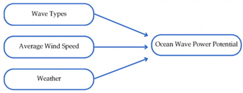
Data processing using R software with attached syntax. The research framework in this study is shown in Figure 3.
Figure 3. Research framework
Hypothesis
The alternative hypotheses used are:
H1: There is an influence between the wave types, average wind speed, and weather to the ocean wave power potential.
Data preprocessing was conducted in R to ensure the quality and reliability of the dataset before analysis. Missing data were identified and addressed using the mice package for multiple imputations, ensuring minimal bias in the dataset. Outliers were detected using boxplots and handled through capping at the 1st and 99th percentiles to reduce the influence of extreme values. Variables were standardized using the scale() function to ensure uniformity in measurement scales, which is particularly critical for regression models. Additionally, categorical variables such as wave type and weather were converted into dummy variables using the model.matrix() function to integrate them into the analysis effectively. The final dataset was verified for consistency, and summary statistics were recalculated to confirm data integrity before proceeding with modeling.
4.1 Descriptive statistics
As a first step, data exploration was conducted to understand the characteristics of the research data. This descriptive analysis is important to determine the distribution, central tendency, and variability of the key variables. Table 2 presents the results of the descriptive statistics of the variables potential power generated and average wind speed, which provide an initial overview of the pattern and relationships in the data.
Table 2. Descriptive statistics
|
Variable |
Min. |
Mean |
Std. Deviation |
Max. |
|
Power Potential |
150,889 |
108,057 |
31,104.48 |
150,889 |
|
Wind Speed |
20 |
9.791 |
3.217353 |
20 |
Figure 4. Wave types pie chart
Figure 5. Wheater pie chart
Based on Table 2, the mean, standard deviation, minimum, and maximum values of the potential power generated and average wind speed variables are obtained in the variable potential power generated obtained and average values of 108,057 with the potential power generated by the average sea wave height in Indonesian waters at least 55,645 Watt and a maximum of 150,889 Watt. The average wind speed variable obtained an average value 9.791 with a minimum value of 4 and a maximum value of 20.
In the wave type variable, there are three categories on May 2, 2024, namely, calm waves, low waves, and high waves. With details, calm waves occur in 29 waters in Indonesia, low waves occur in 99 waters in Indonesia, and moderate waves occur in 47 waters in Indonesia.
In the weather variable, seven types of weather occur on May 2, 2024, in Indonesia waters, namely, partly cloudy, cloudy, heavy cloudy, local rain, light rain, moderate rain, and heavy rain. With details of bright cloudy weather occurring in 30 waters in Indonesia, cloudy weather occurs in 43 waters in Indonesia, thick cloudy weather occurs in 13 waters in Indonesia, local rain weather occurs in 4 waters in Indonesia, light rain weather occurs in 51 waters in Indonesia, moderate rain weather occurs in 32 waters in Indonesia, and heavy rain weather occur in 2 waters in Indonesia.
In addition to the individual pie charts of wave type (Figure 4) and weather (Figure 5), an analysis was conducted to explore the relationship between these two variables. A contingency table was created to examine the frequency distribution of weather conditions across different wave types. The results indicate that low waves are most commonly associated with cloudy conditions, while high waves tend to occur more frequently during heavy rain. Furthermore, a Chi-Square Test showed a significant association (p-value < 0.05) between wave type and weather, suggesting that weather conditions have an observable influence on wave characteristics.
To investigate whether wind speed and weather conditions influence wave types, an additional analysis was conducted. A Chi-Square test was performed to examine the relationship between weather and wave types, which revealed a significant association (p-value < 0.05). Specifically, calm waves were more commonly associated with partly cloudy or cloudy weather, while high waves were observed more frequently during heavy rain. Additionally, a regression analysis indicated that higher wind speeds were significantly correlated with the occurrence of high waves (p-value < 0.01). These results suggest that wind speed and weather indirectly affect power potential by influencing wave types, highlighting their role in shaping wave energy dynamics.
4.2 Generalized linear model analysis
From the previous explanation using the Cullen and Frey graph, it can be concluded that wave power potential by OWC method not normally distributed but are exponentially distributed, tending to have a gamma or beta distribution. Therefore, to analyze the variables that gives a potential to generate renewable energy, the Generalized Linear Model with Gamma link will be used.
The Generalized Linear Model results show that low and medium wave types have a significant negative effect on ocean wave power potential. While other variables such as weather and average wind speed have no significant effect on ocean wave power potential.
Gamma regression data analysis will use Maximum Likelihood Estimation (MLE) parameter estimation. The result of testing the initial model, namely with the predictor variables of maximum wind speed (X1), wave type (X2), and weather (X3) are seen in the Table 3.
Table 3. Gamma regression modeling
|
Parameters |
Estimated Value |
Standard Error |
p-Value |
|
Intercept |
1.797 × 10⁻⁵ |
1.230 × 10⁻²⁰ |
<2 × 10⁻¹⁶ |
|
X1 |
8.818 × 10⁻²³ |
4.738 × 10⁻²² |
0.853 |
|
X2_Low |
-8.270 × 10⁻⁶ |
7.361 × 10⁻²¹ |
<2 × 10⁻¹⁶ |
|
X2_Medium |
-1.124 × 10⁻⁵ |
7.625 × 10⁻²¹ |
<2 × 10⁻¹⁶ |
|
X3_Cloudy |
-2.066 × 10⁻²¹ |
1.095 × 10⁻²⁰ |
0.851 |
|
X3_Cloudy Thick |
-9.952 × 10⁻²² |
1.143 × 10⁻²⁰ |
0.931 |
|
X3_Cloudy Sunny |
5.610 × 10⁻²¹ |
1.104 × 10⁻²⁰ |
0.612 |
|
X3_Heavy Rain |
-2.767 × 10⁻²¹ |
1.784 × 10⁻²⁰ |
0.877 |
|
X3_Local Rain |
-1.441 × 10⁻²⁰ |
1.086 × 10⁻²⁰ |
0.895 |
|
X3_Light Rain |
-1.745 × 10⁻²¹ |
1.116 × 10⁻²⁰ |
0.876 |
|
Null Deviance = 1.6452 × 10 (df = 174) |
Residual Deviance = 1.0535 × 10⁻¹⁴ (df = 165) |
||
Based on the table, the initial model was formed using the predictor variables of average wind speed, wave type, and weather. It was found that the average wind speed and weather predictor variables were not significant. It is necessary to test the model again by excluding the insignificant variables for further model building. Remodeling with average wind speed and weather predictor variables can be seen in Table 4.
Table 4. Gamma regression remodeling
|
Parameters |
Estimated Value |
Standard Error |
p-Value |
|
Intercept |
1.797 × 10⁻⁵ |
8.474 × 10⁻²¹ |
<2 × 10⁻¹⁶ |
|
X2_Low |
-8.270 × 10⁻⁶ |
8.828 × 10⁻²¹ |
<2 × 10⁻¹⁶ |
|
X2_Medium |
-1.134 × 10⁻⁵ |
8.822 × 10⁻²¹ |
<2 × 10⁻¹⁶ |
|
Null Deviance = 1.6452 × 10 (df = 174) |
Residual Deviance = 12.834 × 10⁻¹⁴ (df = 172) |
||
Based on the table, the test results show that the p-value of the wave type predictor variable is less than α = 5% . Therefore, the wave-type predictor variable is significant to the potential power generated. Since there is only one predictor variable in the model, namely wave type, there is no need to test for multicollinearity between response variables.
To evaluate whether a more complex model provides a better explanation than a simpler model, the G2 statistical test has been conducted. This test compares the model fit by considering the difference in log-likelihood between the two models.
Table 5. Model significance test results
|
G2 |
df |
p-Value |
Decision |
|
6126.9 |
2 |
< 2.2e- 16 |
Reject H0 |
Table 5 shows that the p-value is smaller than the value of = 0.05, so it can be concluded that rejecting H0 means that there is a significant difference in fit between the simple model and the more complex model, with the more complex model better explaining the data. So, the full model is better at explaining the data than the reduced model.
Table 6. Final model of gamma regression
|
Parameters |
Parameters |
Estimated Value |
Standard Error |
|
Intercept |
β₀ |
1.797 × 10⁻⁵ |
8.474 × 10⁻²¹ |
|
X2_Low |
β₁ |
-8.270 × 10⁻⁶ |
8.828 × 10⁻²¹ |
|
X2_Medium |
β₂ |
-1.134 × 10⁻⁵ |
8.822 × 10⁻²¹ |
|
Null Deviance = 1.6452 × 10 (df = 174) |
Residual Deviance = 12.834 × 10⁻¹⁴ (df = 172) |
||
After testing the fit of the model using the G2 statistic and finding that a more complex model better explains the data, the next step is to evaluate how well the model predicts the true values. For this, the Root Mean Squared Error (RMSE) is calculated. The RMSE provides a measure of how far away the model predictions are from the observed values, where lower values indicate more accurate predictions and are consistent with previous model fit test results favoring more complex models. The RMSE value obtained from the model with the wave type predictor variable is 2.93e-10. This value shows that the RMSE value is close to 0. So, based on the RMSE value, the prediction results from the model are more accurate or closer to the actual value
By considering the results of the previous stages of analysis, the Gamma regression model was determined as the final model. This model was chosen due to its ability to capture patterns in the data well and provide accurate predictions. The final model obtained from the test results can be seen in Table 6.
Table 6 shows that the effects of the wave-type predictor variable have a very small value. When the wave type variable is 0 and the response variable’s expectation is 1, the exponential value close to one indicates that the value of the response variable or the potential power generated is almost unchanged. When the low waves rise by one unit, the potential power generated will decrease by about 0.0000083% compared to the calm wave. When the medium wave rises by one unit, the potential power generated will decreed by about 0.0000113% compared to the calm wave. This shows a very small decrease in the potential power generated when there is an increase in low or medium waves by one unit compared to calm waves.
This study shows that, although the effect is small, wave type affects the power potential of ocean waves. The OWC technique can be used in Indonesian waters due to its stable performance under various wave conditions. However, it is important to provide further explanation on how the model output is used to assess the power that ocean waves can generate. This includes examining how well the model results show the pattern of energy reliability or maximum power capacity under various wave conditions. In addition, research findings should be linked to their consequences for energy production. This could include the development of more efficient wave power plants or plans to integrate renewable energy into the national energy system. Therefore, further research is needed to find other potential variables.
In addition to the statistical analysis, improvement measures were implemented to enhance the chamber's product efficiency in the OWC system. These measures included optimizing the chamber dimensions and adjusting the airflow outlet to better accommodate wave variability. The chamber width was set at 2.4 meters, reflecting optimal dimensions identified in the prototype used in Pantai Baron, Yogyakarta, Indonesia, with an efficiency rate of 8% [24]. Numerical simulations demonstrated that narrowing the outlet improved air pressure consistency, increasing turbine efficiency. By implementing these adjustments, the chamber's ability to convert ocean wave energy into mechanical energy improved, contributing to the overall effectiveness of the OWC system.
The findings highlight the significant negative impact of low and medium wave types on power potential, which is captured effectively through the Gamma Regression model. This methodological innovation addresses the limitations of linear models used in prior studies, providing a more accurate representation of wave energy dynamics in diverse conditions.
OWC technology for wave power generation has many advantages over hydropower, steam power generation, and solar power generation, especially in terms of sustainability, efficiency, and environmental impact. OWCs use ocean wave energy which is a renewable and stable energy source especially in coastal areas with large waves. The advantage of OWC is its low land footprint as it uses ocean space, which makes it ideal for a country like Indonesia with a long coastline in contrast to Hydroelectric Power Plants that require large dams and can disrupt river ecosystems and Hydroelectric Power Plants that require large dams.
In terms of environmental impact, OWCs are much more environmentally friendly than steam power plants that rely on fossil fuels and produce high carbon emissions. OWCs offer a more sustainable alternative that does not disrupt terrestrial ecosystems. This is in contrast to hydropower plants, which while also renewable, often affect local communities and river flows. Although the initial investment in OWC technology is rather large, as with solar power plants, the operational costs in the long run can be reduced, especially with the technology evolving. In terms of efficiency, OWCs have great potential. This is because, unlike solar power plants that depend on the length of sunlight or hydroelectric power plants that are susceptible to changes in rainfall, ocean wave energy is consistent in a given location. OWCs are an excellent solution to meet the renewable energy needs of small islands and coastal areas and support Indonesia's and the world's energy sustainability targets.
Based on the modelling analysis results, the average potential power generated by ocean waves in Indonesian waters using gamma regression with Maximum Likelihood Estimation (MLE) parameter estimation shows that the wave type factor influences the average potential power generated by ocean waves in Indonesian waters. Meanwhile, the average wind speed and weather factors do not affect the potential power generated by ocean waves in Indonesian waters. The model’s prediction results are accurate because the RMSE value obtained is 2.93e-10, which is close to 0, indicating that the prediction results of the model are very close to the actual values. However, the wave type has minor effect on the potential power generated. When there is one-unit increase in low and medium wave types, the resulting power potential decreases compared to calm waves. However, the decrease that occurs is not too significant. For a low waves, a one-unit increase only reduces the value of the potential power generated by 0.0000083%, and for medium waves, a one-unit increase only reduces the value of the potential power generated by 0.0000113% compared to calm waves.
These results imply that, in comparison to low or medium waves, calm calm waves offer more stable circumstances. Building and running a Marine Wave Power Plant is safer and simpler due to the stability of calm wave conditions, which also lowers the possibility of equipment damage. Moreover, calm waves' consistency and predictability might be helpful for dependable energy generation, even though wave form has little bearing on potential power.
Calm or stable wave condition in Indonesian waters is often observed during dry season, typically from May to September, when the southeastern monsoon wind dominates, resulting in reduced turbulence and consistent sea conditions. These periods provide ideal condition for optimizing the operation of OWC systems, ensuring stable energy generation and minimizing risks associated with equipment stress.
The OWC technology is ideal for areas characterized by flat seabed topography and consistent wave heights, as it requires minimal construction space. In Indonesia, one of the regions that meet these criteria is West Kalimantan, where the coastal waters feature a flat seabed and stable wave conditions. These characteristics make West Kalimantan a promising location for implementing OWC systems. This study aims to provide insights that can assist the West Kalimantan Regional Government in developing policies for establishing Marine Wave Power Plants (PLTGL) in the area.
Considering the model results, the siting and development of Marine Wave Power Plants using OWC should prioritize areas with stable wave conditions, especially during the dry season when the waves tend to be calmer and more predictable. Additionally, based on the model’s findings showing only a minor impact of low and medium waves on potential power, the capacity of OWC systems in areas with low or medium waves can be scaled down to optimize costs without significantly compromising power Bahaefficiency. Maintenance schedules should also be adjusted based on local wave conditions, where systems in areas with more stable waves may require less frequent maintenance, while systems in areas with stronger waves may require more frequent maintenance to ensure optimal operation and prevent damage.
These findings provide the following insights for feature research:
This study used gamma regression with Maximum Likelihood Estimation (MLE) parameter estimation to gather and evaluate data on the power potential produced by ocean waves in Indonesian waters. The average power potential generated in this investigation was found to be influenced by the wave type component, with calm waves exhibiting more stable conditions than low or medium waves. The power potential does, however, slightly drop when wave type varies, indicating a negligible impact of wave type on power potential. By applying a gamma regression model, which can produce precise findings that are near to the true value, the limitations of the available data have been addressed. Additional research is recommended by this study in order to examine the data variability in greater detail and to take various places' wave conditions into account. Additional study with data from more places and longer time periods is needed to gather more thorough information. To ensure the technology's sustainable deployment with an aim to reduce dependence on fossil fuels, thereby lowering greenhouse gas emission and mitigating the effects of climate change, by concentrating on wave energy, a lot emission and renewable energy source.
Compared to traditional energy generation techniques, OWC technology has negligible environmental impact as it does not require much land or emit harmful pollutants. The paper also emphasizes how OWC systems can be incorporated into existing marine infrastructure, which will reduce the demand for new development while protecting marine habitats. However, additional factors that must be considered include environmental impact assessments and the creation of novel technologies for ocean wave energy conversion. In order to validate these results and offer a more comprehensive understanding of the potential of ocean wave power throughout Indonesian waters, future research could involve more thorough and in-depth data analysis.
The authors would like to express their sincere gratitude to Directorate of Research and Community Engagement of Padjadjaran University for their valuable support during the writing of this paper and for providing financial support for publication in this journal.
|
T |
Wave period |
|
H |
Wave height |
|
g |
Earth gravity (9.81 m/s2 ) |
|
E |
Total energy (Joules) |
|
w |
Angular frequency of wave measured (rad/s) |
|
W |
Wald test statistic |
|
N |
Number of data |
|
$x_k$ |
True value |
|
$\hat{y}_k$ |
Predicted value |
|
Greek Symbols |
|
|
$\lambda$ |
Wavelength (distance between two consecutive Wace crests) |
|
$\rho$ |
Water dencity (kg/m3) |
|
$a$ |
Wave amplitude |
|
$\widehat{\beta}_J$ |
Estimator of $\beta_j$ |
|
$S E\left(\widehat{\beta}_J\right)$ |
Standard error of $\beta_j$ |
[1] Sidik, A.D.W.M., Akbar, Z. (2021). Analyzing the potential for utilization of new renewable energy to support the electricity system in the cianjur regency region. Fidelity: Jurnal Teknik Elektro, 3(3): 46-51. https://doi.org/10.52005/fidelity.v3i3.66
[2] Liun, E., Suparman, S., Sriyana, S., Dewi, D., Pane, J.S. (2022). Indonesia’s energy demand projection until 2060. International Journal of Energy Economics and Policy, 12(2): 467-473. https://doi.org/10.32479/ijeep.12794.
[3] Andriyani, T. (2024). UGM Expert Reveals Factors Behind Low Electricity Consumption in Indonesia. Universitas Negeri Gajah Mada.
[4] Pambudi, N.A., Firdaus, R.A., Rizkiana, R., Ulfa, D.K., Salsabila, M.S., Suharno, Sukatiman. (2023). Renewable energy in Indonesia: current status, potential, and future development. Sustainability, 15(3): 2342. https://doi.org/10.3390/su15032342
[5] Yana, S., Nizar, M., Mulyati, D. (2022). Biomass waste as a renewable energy in developing bio-based economies in Indonesia: A review. Renewable and Sustainable Energy Reviews, 160: 112268. https://doi.org/10.1016/j.rser.2022.112268
[6] Setyawan, F.O., Sartimbul, A., Fuad, M.A.Z., Ussania, Q., Hidayatullah, F., Haq, N.A., Satrio, D. (2024). Ocean wave energy potential in southern waters of Malang. In IOP Conference Series: Earth and Environmental Science, IOP Publishing Ltd., p. 012009. https://doi.org/10.1088/1755-1315/1328/1/012009
[7] Junianto, S., Fadilah, W.N., Adila, A.F., Satrio, D., Musabikha, S. (2022). State of the art in floating tidal current power plant using multi-vertical-axis-turbines. In 2022 International Electronics Symposium (IES), Surabaya, Indonesia, pp. 97-103. https://doi.org/10.1109/IES55876.2022.9888749
[8] Yahya, N.Y., Satrio, D. (2023). A review of technology development and numerical model equation for ocean current energy. In IOP Conference Series: Earth and Environmental Science, Surabaya, Indonesia, p. 012019. https://doi.org/10.1088/1755-1315/1198/1/012019
[9] Liguo, X., Ahmad, M., Khattak, S.I. (2022). Impact of innovation in marine energy generation, distribution, or transmission-related technologies on carbon dioxide emissions in the United States. Renewable and Sustainable Energy Reviews, 159: 112225. https://doi.org/10.1016/j.rser.2022.112225
[10] Ribal, A., Babanin, A.V., Zieger, S., Liu, Q. (2020). A high-resolution wave energy resource assessment of Indonesia. Renewable Energy, 160: 1349-1363. https://doi.org/10.1016/j.renene.2020.06.017
[11] Rizal, A.M., Ningsih, N.S. (2022). Description and variation of ocean wave energy in Indonesian seas and adjacent waters. Ocean Engineering, 251: 111086. https://doi.org/10.1016/j.oceaneng.2022.111086
[12] Satrio, D., Widyawan, H.B., Ramadhani, M.A., Muharja, M. (2024). Effects of the distance ratio of circular flow disturbance on vertical-axis turbine performance: An experimental and numerical study. Sustainable Energy Technologies and Assessments, 63: 103635. https://doi.org/10.1016/j.seta.2024.103635
[13] Satrio, D., Adityaputra, K.A., Dhanistha, W.L., Gunawan, T., Muharja, M., Felayati, F.M. (2023). The influence of deflector on the performance of cross-flow savonius turbine. International Review on Modelling and Simulations, 16(1): 27-34. https://doi.org/10.15866/iremos.v16i1.22763
[14] Satrio, D., Albatinusa, F., Hakim, M.L. (2023). The benefit using a circular flow disturbance on the darrieus turbine performance. International Journal on Engineering Applications, 11(1): 55. https://doi.org/10.15866/irea.v11i1.22434
[15] Satrio, D., Albatinusa, F., Junianto, S., Musabikha, S., Setyawan, F.O. (2023). Effect of positioning a circular flow disturbance in front of the darrieus turbine. In IOP Conference Series: Earth and Environmental Science, Surabaya, Indonesia, p. 012019. https://doi.org/10.1088/1755-1315/1166/1/012019
[16] Qiu, S., Liu, K., Wang, D., Ye, J., Liang, F. (2019). A comprehensive review of ocean wave energy research and development in China. Renewable and Sustainable Energy Reviews, 113: 109271. https://doi.org/10.1016/j.rser.2019.109271
[17] Nugraha, I.M.A., Desnanjaya, I.G.M.N., Siregar, J.S.M., Boikh, L.I. (2023). Analysis of oscillating water column technology in East Nusa Tenggara Indonesia. International Journal of Power Electronics and Drive Systems, 14(1): 525. https://doi.org/10.11591/ijpeds.v14.i1.pp525-532
[18] Portillo Juan, N., Negro Valdecantos, V., Esteban, M.D., López Gutiérrez, J.S. (2022). Review of the influence of oceanographic and geometric parameters on oscillating water columns. Journal of Marine Science and Engineering, 10(2): 226. https://doi.org/10.3390/jmse10020226
[19] Sugianto, D.N., Kunarso, K., Helmi, M., Alifdini, I., Maslukah, L., Saputro, S., Endrawati, H. (2017). Wave energy reviews in Indonesia. International Journal of Mechanical Engineering and Technology (IJMET), 8(10): 448-459.
[20] Zikra, M. (2017). Preliminary assessment of wave energy potential around Indonesia Sea. Applied Mechanics and Materials, 862: 55-60. https://doi.org/10.4028/www.scientific.net/AMM.862.55
[21] Suryaningsih, R. (2014). Study on wave energy into electricity in the South Coast of Yogyakarta, Indonesia. Energy Procedia, 47: 149-155. https://doi.org/10.1016/j.egypro.2014.01.208
[22] Rizal, A.M., Ningsih, N.S. (2020). Ocean wave energy potential along the west coast of the Sumatra Island, Indonesia. Journal of Ocean Engineering and Marine Energy, 6(2): 137-154. https://doi.org/10.1007/s40722-020-00164-w
[23] Rahman, Y.A. (2021). The potential of conversion of sea wave energy to electric energy: The performance of central Sulawesi west sea using oscillating water column technology. In IOP Conference Series: Earth and Environmental Science, Bangka Belitung, Indonesia, p. 012073. https://doi.org/10.1088/1755-1315/926/1/012073
[24] Kurniawan, A.T., Budiman, A., Budiarto, R., Prasetyo, R.B. (2022). Wave energy potential using OWC (oscillating water column) system at Pantai Baron, Gunung Kidul, DI Yogyakarta, Indonesia. Journal of Advanced Research in Fluid Mechanics and Thermal Sciences, 92(2): 191-201. https://doi.org/10.37934/arfmts.92.2.191201
[25] Mu’min, A., Gunadin, I.C., Muslimin, Z. (2024). Sea wave energy simulation of oscillating water column (OWC) technology, Binongko Island, Wakatobi, Southeast Sulawesi. In E3S Web of Conferences, Malang City, Indonesia, p. 01010. https://doi.org/10.1051/e3sconf/202447301010
[26] McCullagh, P. (2019). Generalized Linear Models. Routledge, New York, USA. https://doi.org/10.1201/9780203753736
[27] Gao, Y., Zhang, Y., Huang, L. B., Hua, X., Dong, B. (2024). Converting wave scouring damage into opportunities: Advancing marine structure protection through a wave-energy harvesting protective layer. Nano Energy, 123: 109367. https://doi.org/10.1016/j.nanoen.2024.109367
[28] Cong, P., Ning, D., Teng, B. (2024). Enhancement of the energy capture performance of oscillating water column (OWC) devices using multi-chamber multi-turbine (MCMT) technology. Energy Conversion and Management, 322: 119141. https://doi.org/10.1016/j.enconman.2024.119141
[29] Zhang, F., Cong, P., Gou, Y., Sun, Z. (2024). Wave power absorption and wave loads characteristics of an annular oscillating water column (OWC) wave energy converter (WEC) with an attached reflector. Engineering Analysis with Boundary Elements, 169: 105961. https://doi.org/10.1016/j.enganabound.2024.105961
[30] Li, M., Luo, H., Zhou, S., Kumar, G.M.S., Guo, X., Law, T.C., Cao, S. (2022). State-of-the-art review of the flexibility and feasibility of emerging offshore and coastal ocean energy technologies in East and Southeast Asia. Renewable and Sustainable Energy Reviews, 162: 112404. https://doi.org/10.1016/j.rser.2022.112404
[31] Mayon, R., Ning, D., Sun, Y., Ding, Z., Wang, R., Zhou, Y. (2023). Experimental investigation on a novel and hyper-efficient oscillating water column wave energy converter coupled with a parabolic breakwater. Coastal Engineering, 185: 104360. https://doi.org/10.1016/j.coastaleng.2023.104360
[32] Wang, C., Xu, H., Zhang, Y., Chen, W. (2023). Hydrodynamic investigation on a three-unit oscillating water column array system deployed under different coastal scenarios. Coastal Engineering, 184: 104345. https://doi.org/10.1016/j.coastaleng.2023.104345
[33] Qu, M., Yu, D., Xu, Z., Gao, Z. (2022). The effect of the elliptical front wall on energy conversion performance of the offshore OWC chamber: A numerical study. Energy, 255: 124428. https://doi.org/10.1016/j.energy.2022.124428
[34] Medina-Lopez, E., Moñino, A., Bergillos, R.J., Clavero, M., Ortega-Sanchez, M. (2019). Oscillating water column performance under the influence of storm development. Energy, 166: 765-774. https://doi.org/10.1016/j.energy.2018.10.108
[35] Chergui, F., Bouzit, M. (2023). Impact of stepped structures on tsunami wave propagation and overtopping engineering. International Journal of Safety & Security Engineering, 13(4): 753-762. https://doi.org/10.18280/ijsse.130419
[36] Mathew, M.T., Ismail, Z. (2023). Implementing a seismic sensor-driven disaster management system for efficient tsunami early warnings in the Arabian peninsula. International Journal of Safety & Security Engineering, 13(4): 731-737. https://doi.org/10.18280/ijsse.130416
[37] Kavakli, M., Gudmestad, O.T. (2023). Analysis and assessment of onshore and offshore wind turbines failures. International Journal of Energy Production and Management, 8(1): 27-34. https://doi.org/10.18280/ijepm.080104
[38] Pamuttu, D.L., Akbar, M., Andika, A.P., Hariyanto, H. (2023). An investigation of hybrid renewable energy potential by harnessing traffic flow. International Journal of Heat & Technology, 41(1): 239-246. https://doi.org/10.18280/ijht.410126
[39] Malakouti, S.M. (2023). Prediction of wind speed and power with LightGBM and grid search: case study based on Scada system in Turkey. International Journal of Energy Production and Management, 8(1): 35-40. https://doi.org/10.18280/ijepm.080105
[40] Kayesh, M.S., Siddiqa, A. (2023). The impact of renewable energy consumption on economic growth in Bangladesh: Evidence from ARDL and VECM analyses. International Journal of Energy Production and Management, 8(3): 149-160. https://doi.org/10.18280/ijepm.080303
[41] Nelder, J.A., Wedderburn, R.W. (1972). Generalized linear models. Journal of the Royal Statistical Society Series A: Statistics in Society, 135(3): 370-384. https://doi.org/10.2307/2344614
[42] Wedderburn, R.W. (1974). Quasi-likelihood functions, generalized linear models, and the Gauss—Newton method. Biometrika, 61(3): 439-447. https://doi.org/10.1093/biomet/61.3.439
[43] Shrestha, N. (2020). Detecting multicollinearity in regression analysis. American Journal of Applied Mathematics and Statistics, 8(2): 39-42. https://doi.org/10.12691/ajams-8-2-1
[44] Bossio, M.C., Cuervo, E.C. (2015). Gamma regression models with the Gammareg R package. Comunicaciones en Estadistica, 8(2): 211-223. https://doi.org/10.15332/s2027-3355.2015.0002.05
[45] Hodson, T.O. (2022). Root mean square error (RMSE) or mean absolute error (MAE): When to use them or not. Geoscientific Model Development Discussions, 15(14): 5481-5487. https://doi.org/10.5194/gmd-15-5481-2022
[46] Ouali, M.A., Ghanai, M., Chafaa, K. (2020). TLBO optimization algorithm based-type2 fuzzy adaptive filter for ECG signals denoising. Traitement du Signal, 37(4): 541-553. https://doi.org/10.18280/ts.370401