Crude Oil and Economic Performance: Multicollinearity Corrected Approach

Crude oil and oil products serve as a major source of revenue for oil producing nations. The most common hydrocarbon in crude oil is paraffin, also present in all liquid refinery products and part of the process's heavy asphalt-like by-products. Aromatics typically make up a relatively small percentage of most crudes [1]. Nigeria produces the sweetest oil in the Organization of Petroleum Exporting Countries (OPEC), and it is comparable to that of North Sea Oil, and usually classified as light and sweet since it contains little sulfur. In addition to petroleum, Nigeria has natural gas, tin, iron ore, coal, lead, limestone, niobium, and fertile land [2]. Over 90% of the country's earnings were international trade, and 80% of revenue came from oil, which made a significant contribution to the economy's GDP; in the middle of the 1970's crude oil served as the primary source of revenue in Nigeria [3].

Nigeria is a member of OPEC which is a cross-government organization of some developing crude oil exporting countries formed in the 1960s. OPEC's choices on production quotas served as signals to the market about the desired range of prices; however, the strength of the signals depended on the market's perception of OPEC's ability to alter production in response to market circumstances [4].

Historically, Nigeria significant source of income and earnings in foreign currencies comes from crude oil. According to the study [5], the oil and gas industry contributes almost 10% to the Gross Domestic Product (GDP), and almost 86 percent of all export earnings come from the sale of petroleum products. On the other hand, in 2016, the economy experienced its first economic decline in 25 years due to a combination of falling oil prices worldwide, which hit a 13-year low, and a decline in oil production brought on by militant attacks and vandalization of oil pipeline in the Niger Delta. The event led to a sharp contraction in the GDP of the oil sector. Through the channels of money and currency rates, this underperformance in the oil sector spread to the non-oil sector of the economy [6]. The oil industry is Nigeria's most prominent economic driver; and ranked tenth largest producer of oil in the world and the third-largest producer in Africa. The country's foreign exchange revenue is 95% derived from its oil reserves ranging from 24 billion dollars to 31.5 billion dollars [7].

The early 1980s saw a glut in the global oil market, which reduced export profits in foreign currency and rendered the nation's import-dependent structure unsustainable; this resulted in the adoption of several policy initiatives, which comprised the Stabilization Act of 1982, a strict monetary policy and strict exchange rate control measures in 1984, all of which proved ineffective at the end. The Structural Adjustment Programme (SAP) was then implemented in 1986 which prepared the ground for the complete liberalisation of the Nigerian economy, to create a competitive business environment for the manufacturing sector [8, 9]. One of the components of SAP was the export promotion industrialization policy. The policy is intended to encourage both agricultural and industrial output for exports. Nevertheless, the non-oil exports performed poorly after that, although the country's overall output, as measured by its Gross Domestic Product (GDP), had steadily risen [10], as study [11] asserts that export is a foundation and the driver for economic growth. Without a doubt, crude oil exports have been a notable source of income for the economy over the years, and their influence on the economic growth and development of oil-producing nations, cannot be over-emphasized. The study [12] investigated the effect of crude oil price shocks on the economic growth of nine selected countries using the Autoregressive Model. The study showed that crude oil prices impacted economic growth positively. The study identified some challenges in the countries and suggested that the countries should improve on some macroeconomic policies such as fiscal and monetary policies.

A related but different approach includes researcher [13] who applied a synthetic control technique to study the effect of the sharp decline in oil prices on oil-rich countries oil-producing countries. The study demonstrated that oil volatility negatively impacts the economy and the financial institutions. The authors strongly drew the attention of policymakers to the positive role of financial development in fostering growth and improving energy security. Other related studies include researchers [14-18]. The current study seeks to identify how much the oil sector have imparted on the economic growth of Nigeria.

The studies that are related to economic growth in the Nigerian context include that of study [19], which is among the few studies available in the literature that contain more than two variables. The study considered the impact of Capital, Labour, Real Gross, crude oil export, Domestic Product, and crude oil consumption in Nigeria from 1970 to 2005. The study showed that crude oil impacted the economic development of Nigeria. Despite the favourable impact of crude oil on economic development, the study concludes that crude oil production (for Consumption and export) has not greatly enhanced economic growth due to administrative shortcomings. Another related study [20] was to determine how susceptible the economy of an oil-producing nation was to changes in oil prices, using Nigeria. The study identified a significant impact of crude oil on economic development. Despite the massive earnings from oil, the Nigerian economy continues to face some challenges, including an increasing unemployment rate, declining production output, neglect of the agricultural sector and low earnings. The oil sector in Nigeria has received so much attention in the past decades, and it is important to identify various factors that enhances its growth or otherwise. However, there are activities mitigating revenue maximization at the same time impacting on the Real Gross Domestic Product which is a metric for economy growth [19].

Relative to existing studies in literature, the current study uses the Cobb-Douglas production function (Non-linear) to determine the relationship between Real GDP and some crude oil variables, and employ multicollinearity checks on the regressors. A non-linear model can either be an intrinsically Linear Model or a non-intrinsically Nonlinear Model. When a model is nonlinear, but can be transformed to become linear, such model is referred to as an intrinsically non-linear model; otherwise, it is a non-intrinsically non-linear model [21]. Study [22] applied the Cobb-Douglas production function to estimate the variables affecting the productivity of small-scale fishermen. The application of the model helped to draw useful inferences from the data obtained. Previous study [23] also applied Cobb-Douglas to the level of component productivity in banking. The model was also applied to analyse Poland's Economy [24]. The authors examined the connection between global commerce and Poland's economic and financial development. The model was considered suitable for the study and insightful inferences were drawn. Another study where the Cobb-Douglas model was applied is in the determination of the technical and economic efficiency of cement production in Nigeria [25]. The study demonstrated that the Cobb-Douglas Production function was suitable for modelling the data and identified significant relationships among the variables of interest namely labour, capital and material. The studies of [26-33] provided the mathematical base, and areas of applications of the Cobb-Douglas model.

As mentioned earlier, an intrinsically non-linear model becomes linear after taking the log (log-linear), hence could potentially suffer the problem of multicollinearity depending on the nature of the data. Multicollinearity occurs when a predictor variable in a multiple regression model can be correctly predicted linearly from the others. The multiple regression correlation coefficient estimates in this situation may vary erratically due to slight modifications to the model or data. Multicollinearity only impacts calculations about specific predictors; it has no impact on the predictive capability or reliability of the Model within the data set. Multicollinearity is the term used to denote the relationship between two or more linear explanatory variables.

No recent studies had been conducted on the crude oil and economic performance in Nigeria, hence the need for the current study. The current study utilizes a non-linear (log-linear) model, namely the Cobb-Douglas model to analyse the petroleum data. The remaining part of this study is structured into three sections, the second section provides the material and methods, followed by the results and discussion in the third section and the last section is the summary and conclusion.

In this session, the results of the analyses carried out are presented accordingly. Table 2 contains the correlation matrix of the data. The econometric method in this research considers the variables, crude oil export, crude oil consumption, crude oil revenue, and Petroleum to GDP as the independent variable and Real Gross Domestic Product as the dependent variable. They were used to obtain a reliable estimate in the regression model. The correlation coefficient of the data is presented in Table 2.

Table 2. Correlation coefficient of Nigerian crude oil data

Table 2 shows the correlation coefficients of the variables in the data.

The results show that there is a strong positive correlation between crude oil revenue and crude oil export, which shows that increase crude oil trade increases revenue. Crude oil revenue also had a positive relationship with RGDP and PGDP. COC has a positive relationship with crude oil revenue.

Table 2 also shows that COC has positive relationship with crude oil export, PGDP and RGDP. Crude oil export has a low positive relationship with both PGDP and RGDP showing that crude oil export impacts on economy of Nigeria, though reveal low relationships. Finally, from Table 2, PGDP and RGDP have a very low negative relationship (-0.0767). The Augmented Dickey-Fuller test for stationarity was conducted on all the data. Alternative hypothesis: data is stationary, while the null hypothesis: the data has unit root. The test results are discussed as follows.

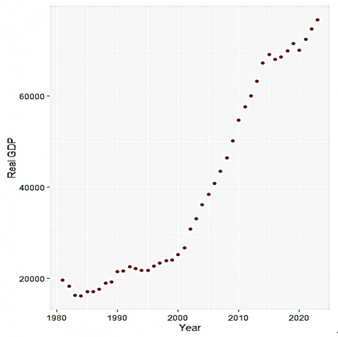
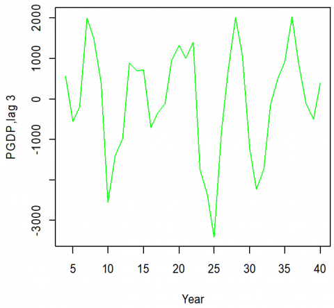
Figure 1 is the plot of the raw data. It shows a steady Real Gross Domestic Product from 1980 – 2000, followed by a consistent increase from 2005 – 2015 and somewhat stable from 2015 – 2020, the consistent increase between 2005 to 2015 could be attributed to some factors such as Economic growth, Consumer spending, Employment opportunities and Increased investments. Figure 2 is the plot of RGDP at lag 3, after conducting a stationarity test with the Augmented Dickey-Fuller test (-1.7698) p-value = 0.6646. Since alpha is greater than 0.05, we fail to reject the null hypothesis of unit root. The results show that the data of RGDP is stationary at lag 3.

001.png

Figure 1. Plot of Real GDP versus year

002.png

Figure 2. Plot of Real GDP differenced at lag 3

Figure 3 is the plot of raw data of Petroleum to GDP, which shows variations in the Petroleum to GDP over time, with increases, decreases and the changing nature of the data points, indicating the ratio is not constant and experiences change over the years. Here are some possible causes for the increase and decrease, Oil Prices, Production levels, Demand for Petroleum products and Economic conditions. Figure 4 is the plot of PGDP at lag 3, after conducting a stationarity test with the Augmented Dickey-Fuller test (-1.1057) shows that the data of PGDP is stationary at lag 3, p-value = 0.9105. Since alpha is greater than 0.05, we fail to reject the null hypothesis of unit root. The results show that the data of RGDP is stationary at lag 3.

003.png

Figure 3. Plot of PGDP versus year

004.png

Figure 4. Plot of PGDP differenced at lag 3

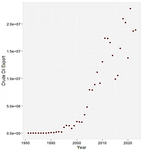
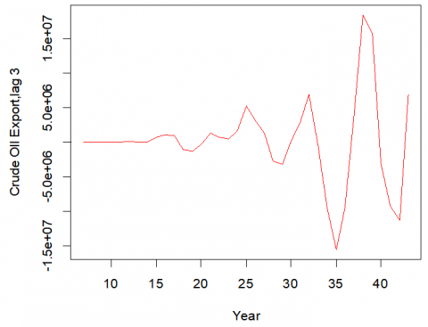
Figure 5 is the plot of the raw data, shows that there was a period of low exports, followed by significant growth, then a more dynamic trend with fluctuations in the amount of crude oil exports (barrels) in the later years, the reasons for this fluctuation could be related to market conditions, production levels and government policies, among others. While Figure 6 is the plot of crude oil export at lag 3, after conducting a stationarity test with the Augmented Dickey-Fuller test (-2.3156) p-value = 0.4490. Since alpha is greater than 0.05, we fail to reject the null hypothesis of unit root. The results show that the data of RGDP is stationary at lag 3.

005.png

Figure 5. Plot of crude oil export versus year

006.png

Figure 6. Plot of crude oil export differenced at lag 3

Figure 7 shoes that from 1981 to 1990, crude oil consumption remained at around 14 million metric tons per year, however, there was a significant spike and consumption increased to about 80 million metric tons per year in 1997. Nigeria experienced economic growth in the 1980s was occasioned by industrial growth between 1981 to 1990 which necessitated the increase in demand of petroleum products. Nigeria attracted more investors in textile, wood and wood products, Metals and metal products, chemical, to mention but a few. Speedy industrialization received priority in Nigeria’s development objectives [34]. The significant spike in crude oil consumption was also due to the need for people to power generators for homes and businesses and increase in demand of petroleum products due to the acquisition of privately owned vehicles. It came down to about 10 million metric tons per year in 1999, the consumption was relatively stable until 2011 when there was another increase, and the consumption rose back to about 70 million metric tons per year. The period of stable consumption, significant spikes and declines could be influenced by shifts in global demand for petroleum products, technological factors or changes in energy policies. Figure 8 is the plot of crude oil consumption at lag 3, after conducting a stationarity test with the Augmented Dickey-Fuller test (-3.6503), p-value = 0.04064. Since alpha is less than 0.05, we reject the null hypothesis in favour of the alternative hypothesis that the data of crude oil export is stationary at lag 3.

007.png

Figure 7. Plot of crude oil consumption

008.png

Figure 8. Plot of crude oil consumption differenced at lag 3

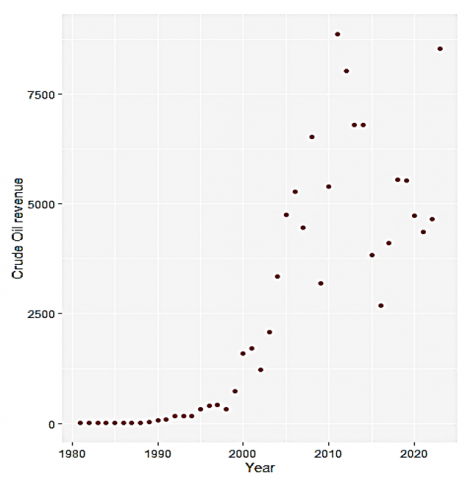
Figure 9 is the plot of the raw data; the plot shows that between 1981 and 1991 crude oil revenue were not so much but started picking up from 1992. Figure 9 shows how crude oil revenue fluctuated throughout the observed period. There were periods of slow and large growth rate of revenue. It also indicates that crude oil revenue showed irregular variations, both increase and decrease over the years.

009.png

Figure 9. Plot of crude oil revenue

Figure 10 is the plot of crude oil revenue at lag 3, after conducting a stationarity test with Augmented Dickey-Fuller test (-2.4694) p-value=0.3883. Since alpha is greater than 0.05, we fail to reject the null hypothesis of unit root. The results show that the data of RGDP is stationary at lag 3. The result of the full model is presented in Table 3 as follows:

010.png

Figure 10. Plot of crude oil revenue differenced at lag 3

Table 3. Estimates using the full model

---Sig. codes: 0 ‘***’ 0.001 ‘**’ 0.01 ‘*’ 0.05 ‘.’ 0.1

The second column of the upper part of Table 3 is the coefficient estimate of the model and present in a log-linear form in Eq. (9) based on Eq. (2).

$\begin{aligned} &log \widehat{R G} D P=19.2599+0.2744 log R +0.0411 log C+0.0039 log E -1.28951 log P\end{aligned}$      (9)

Table 3 shows the results of the full model. The intercept, log (COR), log (COC), and log (PGDP) significantly impact Real GDP at a 0.05 significant level. R-squared is 0.9148, which shows that 91.48% variation in the response variable results from the independent variables included in the Model. Adjusted R-squared: 0.9059, $F$ Statistics is 102.1, p-value<2.2e-016 and its significant at 1%, which shows that the model is highly significant. Table 4 shows the multicollinearity diagnostics for the full model.

Table 4. Overall multicollinearity diagnostics for the full model

If multicollinearity is detected, the ‘detection’ column for each metric is 1, and if ‘detection’ is 0, it means that collinearity is not detected. The results showed that based on the Determinant |$X^{\prime} \boldsymbol{X}$|, Chi-Square, Red Indicator Sum of Lambda Inverse (SLI) metric, multicollinearity was detected since they have a value of “1”. From Table 4, there is the presence of multicollinearity among the regressors. We then proceed to VIF checks to determine the regressors causing high collinearity. Table 5 shows the VIF multicollinearity test on the full model.

Table 5. Multicollinearity test (VIF) for full model

From Table 5, the VIF of log (COR) and log (Export) is high with 97.7230 and 85.7685 respectively, and these values are greater than 10 as mentioned in section 2.2. It shows that the variables have high linear relationships and hence the best linear unbiased estimator assumption is violated, and the results could be misleading. We remove these variables and re-run the analysis. Table 6 shows the estimates after removing variables responsible for multicollinearity.

Table 6. Estimates after removing variables responsible for Multicollinearity

The second column of the upper part of Table 3 is the coefficient of the model and present in a log-linear form in Eq. (10).

$\begin{aligned} &log \widehat{R G} D P=-4.9920+0.3822 log C+1.0494 log P\end{aligned}$       (10)

Table 6 shows the results of the reduced model. R-squared is 0.4612, which shows that 46.12% variation in the response variable results from the independent variables included in the Model, adjusted R-squared is 0.2975. The $F$ Statistics is 9.891; p-value is 0.0003234, the significant at 1%. Both log (COC) and log (PGDP) are significant at 1% alpha level indicating a very strong relationship whereas log (COC) was not significant in the full model, Table 7 is the overall multicollinearity diagnostics for the reduced model.

Table 7. Overall multicollinearity diagnostics

Table 7 shows that collinearity is not detected based on the Determinant |$\boldsymbol{X}^{\prime} \boldsymbol{X}$|, Chi-Square, Red Indicator Sum of Lambda Inverse (SLI) metric, multicollinearity was not detected since all the values in the column “detection” is 0. We proceed to VIF test presented in Table 8.

Table 8. Multicollinearity test (VIF)

From Table 8, the VIF for the remaining variables are lower than 5, implying that the result obtained is reliable and the Best linear unbiased estimate condition has not been violated.