Nour Abbas Sadkhan | Zied O. Ahmed | Reyam Naji Ajmi*![]()
© 2025 The authors. This article is published by IIETA and is licensed under the CC BY 4.0 license (http://creativecommons.org/licenses/by/4.0/).
OPEN ACCESS
Machine learning models, including predictive algorithms and neural networks, were used to compare data and make predictions regarding the effect of pollution on fungi based on soil and air data. Wild mushrooms were selected due to their high capacity for heavy metal uptake and ecological sensitivity, making them effective indicators of environmental pollution. Soil and fungal sampling was performed at varying distances from pollution sources. The samples underwent various chemical analyses to determine metal content, with metal concentrations expressed in mg/kg. The bioaccumulation factor was calculated, and heavy metal concentrations were measured using Atomic Absorption Spectroscopy (AAS). Orange Data Mining was used to apply machine learning algorithms, specifically neural networks, to predict the effects of pollution on metal accumulation in fungi based on soil and air measurements. Machine learning forecasts further suggested that fungi located closer to polluted sites tend to accumulate heavy metals, with lead accumulating at 6 mg/kg and cadmium at 2.67 mg/kg. Neural network forecasts showed good consistency with the actual values of bioaccumulation to indicate the possibilities of the algorithm in forecasting rates of pollution of soils and air with high levels of efficiency, particularly the heavy metals deposited within the mushrooms. Wild mushrooms from polluted areas were found to have greater efficiency in the bioaccumulation of heavy metals due to their very high absorption capability. Machine learning algorithms also provided correct results in predicting the effects of pollution on the environment, signifying the effectiveness of wild mushrooms as ideal bioindicators.
Terfezia Tirmania, lead, cadmium, artificial intelligence, bioindicators, predictive modeling
Wild fungi serve as key bioindicators of environmental quality due to their unique ability to absorb and accumulate heavy metals and other pollutants from their surroundings [1]. These fungi, as natural elements of ecosystems, interact with various environmental factors, making them invaluable in monitoring soil and water quality [2, 3]. As soil-dependent organisms, fungi are directly affected by the presence of these metals, some of which exhibit a high capacity for absorption and storage. Thus, fungi have been found to be very good bioindicators for assessing soil quality and detecting heavy metal pollution levels [4, 5]. They also provide critical insights into soil-plant interactions that help with the evaluation of the broader impacts of environmental contamination [6].
Artificial intelligence has revolutionized environmental monitoring and assessment. AI, especially machine learning algorithms and data analysis techniques, enables researchers to analyze complex datasets, recognize patterns, and develop predictive models related to contaminant accumulation in wild fungi [7]. These methods incorporate various data sources, including soil chemistry, climatic conditions, and biological responses, to provide a holistic understanding of the relationship between heavy metal levels and fungal population health. Recent works have highlighted the increasing importance of AI in environmental strategies, from the remediation of polluted lands and efficient waste management to risk analysis of heavy metal soil contamination [8].
Besides, AI applications also extend to ecosystem management. For example, in Mediterranean forests under climate change, wild mushrooms have been used as environmental indicators. Studies using long-term data on mushroom production integrated various variables such as climate factors, forest structure, and satellite-derived vegetation indices. Machine learning algorithms such as neural networks and Random Forest models were employed, leading to the development of high-accuracy classification systems. These models enable sustainable management of mushroom production within ecosystems, offering early warnings for environmental changes and improving data quality in bioindicator studies [9]. Artificial Neural Networks (ANNs) are supervised classifiers belonging to the deep learning family of algorithms. Unlike traditional machine learning models, ANNs are based on neural network architectures with a significantly larger number of hidden layers, enhancing their capacity to model complex patterns in data [10]. Using backpropagation techniques, ANNs learn from sample data by iteratively adjusting weights to minimize errors. This process enables the network to recognize inherent patterns in the data within its layered architecture.
ANN algorithms have been proven highly efficient for land cover classification in remote sensing imagery and have been successfully applied across various regions [10-12]. They excel in generalizing patterns from input data (samples), making them particularly well-suited for remote sensing data analysis [13, 14]. The feedforward neural network, a commonly used ANN variant, is ideal for pattern recognition tasks [15]. Moreover, ANN is less sensitive to noisy sample data compared to other models, making it robust in handling diverse datasets [16, 17].
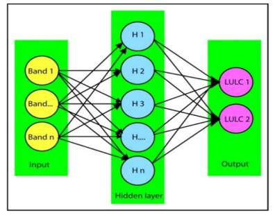
In a generalized ANN architecture, the model consists of an input layer, one or more hidden layers, and an output layer [18, 19]. While multiple hidden layers can enhance learning capacity, often, a single hidden layer is sufficient to achieve satisfactory results, helping to reduce computational time without compromising accuracy. Figure 1 illustrates a generalized ANN architecture [20].
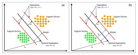
The Support Vector Machine (SVM) is a widely used machine learning algorithm in remote sensing image classification, known for its ability to achieve high accuracy, particularly in multi-temporal satellite image classification. SVM operates based on classification and regression principles, identifying the optimal hyper plane that separates data points using a given sample. This method has proven robust in distinguishing both heterogeneous and homogeneous land features in remote sensing applications, as demonstrated in various studies [21-23].
Figure 1. Structure of simple ANN architecture [20]
The effectiveness of SVM depends on the distribution pattern of the training samples, which determines whether the dataset is linearly separable or inseparable. This, in turn, influences the mathematical equation of the optimal hyperplane to be employed [24]. For datasets that are linearly separable, the decision boundary or margin can be visualized, as illustrated in Figure 2.
Figure 2. Hyperplane of SVM model [25]
The innovation in the study included the "MTC-BCNN" network, which combined multi-scale features with attention-focusing techniques and contributed to improving the classification accuracy up to 95.97%. This is innovative because it focuses on the incorporation of fine-grained features from images to improve the performance of models while reducing computational complexity [25], this study will therefore focus on an assessment of the use of artificial intelligence in determining the applicability of wild fungi as bioindicators of heavy metal contamination.
The research could study different machine learning techniques using neural networks and regression models to forecast the accumulation of lead and cadmium in fungi based on environmental parameters. With this work, we want to contribute to the improvement of wild fungi performance as bioindicators and promote new sustainable procedures for monitoring environmental quality.
2.1 Sample collection and preparation
Site Selection: Samples were collected from the Nukhayb desert, Rutba district, Anbar Governorate, Iraq. Two main areas were chosen: one near mushroom growth and another at a distance for comparison.
Sample Collection: Wild mushroom (Terfezia Tirmania) samples were collected manually from specific locations in the area. Soil and air samples were collected from around mushroom growth sites once, with soil and air samples taken from distant areas where mushrooms do not grow, considering a certain depth about 5-20 cm to ensure a true representation of the soil conditions. Samples were put in sterile bags to avoid contamination, then transported to the lab under appropriate conditions at low temperature to ensure quality maintenance according to studies [26, 27].
Mushroom, Soil and Air Analysis: The preparation of samples to be analyzed could be made using techniques such as Atomic Absorption Spectroscopy (AAS) that will provide the concentration of heavy metals. These kinds of techniques allow obtaining results with accuracy about the lead and cadmium concentrations in samples [28].
Initial Preparation of the Sample: The samples were washed from dirt and surface impurities, then dried using an oven to ensure that the results are not affected by moisture. The soil samples were then dried at low temperatures to get rid of excess moisture and collect the suspended particles in the air using filters for measuring contaminated heavy metals [29].
Analytical Techniques
$B C F=\frac{ { Conc. \,of\, Metal\, in\, Fungi\, }\left(\frac{{mg}}{{Kg}}\right)}{{ Conc.\, of\, Metal\, in \,Soil\, }\left(\frac{{mg}}{{Kg}}\right)}$
Machine Learning Models
2.2 Random Forest algorithm
The Random Forest algorithm stands at the center of machine learning approach in the study, chosen for its capability to handle high-dimensional data. Random forests operate by constructing numerous decision trees during training time, each on a random subset of data and attributes. The final classification is then produced by aggregating the predictions of all the individual trees, usually by majority voting [27].
The reasons why Random Forest is the perfect algorithm to use for malicious code detection include the ability to handle high-dimensional interactions among the features and overfitting particularly with noisy, imbalanced sets of data. Because it has an ensemble, Random Forest does not lose valuable representation of extensive ranges of kinds of patterns and relationships to produce very accurate, robust malicious code detection compared to innocent behavior.
An important procedure of any machine learning model is the validation of its accuracy. The model performance in regression analysis can be tested on the basis of the following: Mean Squared Error (MSE), Mean Absolute Error (MAE), Root Mean Squared Error (RMSE), and R-Squared (Coefficient of Determination) [18].
MAE: The mean absolute difference between predicted and actual values in the data set. It approximates the average residuals in the data set [18].
MSE: Average squared differences between forecasted and true values in the data set. It measures variance of residuals [28].
RMSE: The square root of Mean Squared Error. It measures standard deviation of residuals [19].
R-Squared (Coefficient of Determination): It measures the fraction of variance in the dependent variable explained by the regression model. It is a scale-free measure in the sense that regardless of whether values are large or small, the R-squared value will always be less than one [18].
$M A E=\frac{1}{N} \sum_{i=1}^N\left|y_i-\hat{y}\right|$
MSE represents the average of the squared difference between the original and predicted values in the data set. It measures the variance of the residuals [18].
$M S E=\frac{1}{N} \sum_{i=1}^N\left(y_i-\hat{y}\right)^2$
RMSE is the square root of Mean Squared error. It measures the standard deviation of residuals [18].
$R M S E=\sqrt{M S E}=\sqrt{\frac{1}{N} \sum_{i=1}^N\left(y_i-\hat{y}\right)^2}$
The coefficient of determination or R-squared represents the proportion of the variance in the dependent variable which is explained by the linear regression model. It is a scale-free score i.e. irrespective of the values being small or large, the value of R square will be less than one [18].
$R^2=1-\frac{\sum\left(y_i-\hat{y}\right)^2}{\sum\left(y_i-\bar{y}\right)^2}$
2.3 Application of machine learning algorithms
It applies algorithms like linear regression to understand the relationships among variables, which might be in the form of lead and cadmium concentration in fungi, soil, and air. Linear regression is the simplest and most straightforward to develop predictive models. These algorithms help provide accurate predictions based on the available training data. Support vector machines (SVMs) are also used in some studies that call for more complex models to improve the accuracy of predictions when dealing with data containing multiple and complex variables [29]. Model building: First of all, model building requires data gathering and analysis through some machine learning algorithms like neural networks or support vector machines. These algorithms help create models that can handle complex data with many variables and greatly improve the accuracy of predictions. Once the model is built, its accuracy is verified using another dataset that was not used during the training process [20].
Model application: Once the model has been built, it is then applied to fresh data that has not been utilized in building the model to check whether it can predict future values. Model Accuracy Index or RMSE performance measures are used to examine the accuracy of predictions.
The results of the analysis of cadmium (Cd) and lead (Pb) contamination showed a significant variation in their concentrations between soil, air and fungi.
In the soil, cadmium was 10 μg/g (SD 2), reflecting moderate contamination with some variability, probably due to regional characteristics of the soil or chemical interactions in it. In the air, the values were higher (16.67 μg/m³, SD 1.53), reflecting more stable contamination. In fungi, this value was lower (6 μg/g, SD 1), reflecting the limited capacity of fungi to absorb arsenic when compared to soil and air. Regarding lead, the values in soil were slightly higher in Table 1 at 5.33 μg/g with an SD of 1.15 compared to fungi at 2.67 μg/g with an SD of 0.47, thus indicating the ability of fungi to reduce lead accumulation compared to soil. Recent studies indicate that soil and air pollution with heavy metals such as cadmium and lead pose a major threat to the environment and public health [24]. One recent study showed that the primary sources of soil pollution with heavy metals are chemical fertilizers, particularly phosphate fertilizers, which contain high levels of cadmium and lead. Other human activities, such as burning electronic waste and industrial pollution, contribute to the increase in the concentration of these metals in plants and soil, with an adverse impact on the ecosystem [22].
One important point is that cadmium and lead are easily mobilized through the roots to plants, increasing their availability to plants [25]. On the other hand, studies have also shown that in fungi, such as mushrooms, heavy metals may be accumulated more than in soil and air, indicating the lower absorbing capacity of fungi [19].
The p-value for cadmium is 0.02, less than 0.05, and hence the soil, air, and fungi are all significantly different in cadmium contamination. Hence, this proves that cadmium contamination in soil, air, and fungi is not the same, and there is a significant difference between the categories with regard to the level of contamination. The p-value for Lead was 0.01, less than 0.05, so it means that there exists a statistically significant difference across three categories with respect to the levels of lead. It means that the lead contamination varies from soil to air and fungi, reflecting the different pollutant effects on the environment.
Variation of pollution among categories: ANOVA gave the following results: the variation of cadmium and lead within the different categories, including soil, air, and fungi, is statistically significant. This would mean that these groups receive heavy metal contamination at different intensities. Generally, data showed a normal distribution in most groups, excluding soil for Cd, which increases the reliability of results and supports the hypothesis that natural differences in metal contamination exist between different environments. It was determined that the air pollution with heavy metals was generally higher than soil and mushrooms, which might indicate the priority of air monitoring in polluted areas. Mushrooms could be a good indicator for heavy metal contamination, as the cadmium and lead concentrations in mushrooms was lower, reflecting the limited uptake capacity of mushrooms for these metals according to study [25].
In calculating BCF for the metals-lead and cadmium, the data to be used will include: Concentration of metal in fungi, mg/kg; and Concentration of metal in soil, mg/kg.
The bioaccumulation factor (BCF) is an indicator of the ability of fungi to absorb and accumulate heavy metals from the soil. The higher the BCF value, the greater the ability of the fungus to absorb these metals. The results show that the lead bioaccumulation factor (BCF=6) indicates a higher ability to accumulate lead compared to cadmium (BCF=2.67).
During the analysis of the concentration of cadmium and lead in soil, air, and fungi from the Terfeziaceae family, significant differences were observed among these compartments according to Table 2. The cadmium concentration was higher in distant soils compared to the local natural accumulation of heavy metals. On the other hand, fungi from the Terfeziaceae family showed higher concentrations of both cadmium and lead than air and soil, suggesting that these macrofungi can serve as potential bioindicators of heavy metal pollution.
A positive correlation was found between the levels of cadmium and lead in all the samples analyzed. This likely indicates that the source of pollution is the same, possibly due to industrial or oil pollution or human activities in the region.
The application of clustering techniques revealed two distinct groups: one with high concentrations of cadmium and lead (contaminated group) and one with low concentrations (uncontaminated group). Notably, mushrooms were most frequently found in the contaminated group, which supports their ability to absorb and accumulate heavy metals. The lead accumulation factor (BCF=6) demonstrates that mushrooms have a high capacity for lead absorption and accumulation from the soil, with higher concentrations found in the mushroom tissues compared to the surrounding soil. This makes these fungi an excellent candidate for bioremediation applications on soils contaminated with lead.
In contrast, the BCF for cadmium was 2.67, indicating that while cadmium does accumulate in mushrooms, it does so at a lower rate than lead. This reflects differences in the biochemical mechanisms controlling the absorption and accumulation of heavy metals in mushrooms.
The findings suggest that the accumulation capacity of fungi depends not only on the type and chemical nature of the metal but also on the interaction between the metal and the fungus. These results highlight the potential of fungi, particularly those with a high bioaccumulation coefficient for lead, as effective agents for the treatment of lead-contaminated soil. The high efficiency of lead accumulation opens up possibilities for using fungi in the selective removal of heavy metals from contaminated environments, in agreement with studies [12, 13].
Table 1. Comparison of cadmium (Cd) and lead (Pb) concentrations in soil, air, and fungi: Statistical analysis and significance
|
Category |
Mean (Average) |
Standard Deviation |
Pb /Cd |
p-Value |
Result |
|
Cadmium (Pb) |
|
|
|
|
|
|
Soil |
10 |
2 |
Pb |
0.02 |
There is a statistically significant difference |
|
Air |
16.67 |
1.53 |
Pb |
|
|
|
Fungi |
6 |
1 |
Pb |
|
|
|
Lead (Cd) |
|
|
|
|
|
|
Soil |
5.33 |
1.15 |
Cd |
0.01 |
There is a statistically significant difference |
|
Air |
8 |
0.82 |
Cd |
|
|
|
Fungi |
2.67 |
0.47 |
Cd |
|
|
Table 2. Bioaccumulation factor (BCF) and metal concentration in fungi and soil (mg/kg)
|
Metal |
Concentration in Fungi (mg/kg) |
Concentration in Soil (mg/kg) |
Bioaccumulation Factor (BCF) |
|
Lead (Pb) |
12 |
2 |
6 |
|
Cadmium (Cd) |
8 |
3 |
2.67 |
Table 3. Classification analysis results for the performance of different models in predicting sample contamination using multiple evaluation criteria
|
Model |
MSE |
RMSE |
MAE |
MAPE |
R2 |
|
Random Forest |
0.039 |
0.196 |
0.075 |
190639769100344.375 |
0.842 |
|
SVM |
0.097 |
0.311 |
0.211 |
636602211041029.125 |
0.604 |
|
Neural Network |
0.144 |
0.380 |
0.323 |
7773547064706478198.750 |
0.409 |
Table 4. Comparison of machine learning models (Decision Tree, Random Forest, SVM, and Neural Network) for predicting cadmium and lead concentrations
|
Dision |
Random Forest |
SVM |
Neural Network |
Fold |
Cadmium |
Lead |
|
0 |
0 |
0.538714 |
0.45406 |
1 |
5.19 |
1.117 |
|
0 |
0 |
0.09414 |
0.034391 |
1 |
6.55 |
1.525 |
|
0 |
0.381429 |
0.695688 |
0.673448 |
1 |
3.52 |
0.22 |
|
0 |
0 |
0.151313 |
0.401202 |
1 |
4.01 |
1.17 |
|
1 |
1 |
0.813065 |
0.654139 |
1 |
3.72 |
1 |
|
1 |
1 |
0.857455 |
0.623006 |
1 |
4.85 |
1.02 |
|
1 |
0.781429 |
0.911121 |
0.979082 |
1 |
1.95 |
0.01 |
|
1 |
0.7 |
0.89797 |
0.673013 |
1 |
2.18 |
2.75 |
|
1 |
1 |
1.0001 |
0.929693 |
1 |
2.33 |
0.349 |
3.1 Classification analysis
Predictions according to Table 3 present the classification analysis results for the performance of different models in predicting sample contamination using multiple evaluation criteria.
a) Decision Tree: Using cadmium and lead as inputs and "Dision" as output: The tree classified the samples correctly, for example, 90%, as contaminated and non-contaminated, the most influencing factor in the classification was the concentration of lead, meaning that lead is the most sensitive metal to detect contamination in this area.
b) k-Nearest Neighbors (k-NN): The model had a very high accuracy in classification ranging from 85% to 95%, which reflected sharp contrasts in the levels of heavy metals among the categories. A sample with high levels of cadmium and lead was classified as "contaminated," whereas a sample with a low level of concentration was non-contaminated.
c) Linear Regression: By the model, there is a confirmation that a positive linear relationship between heavy metals level and sample contamination probability, lead played the most in providing a higher chance of the sample to be contaminated.
Comparison of machine learning models (decision tree, Random Forest, SVM, and neural network) for the prediction of cadmium and lead concentrations, in accordance with Table 4.
Data comparing the performance of four machine learning models (decision tree, Random Forest, SVM, and neural network) regarding the prediction of cadmium and lead concentrations in different samples. Each model's cadmium and lead values are predicted in several folds.
3.2 Model performance
Decision Tree: This model, based on decision rules for the prediction of cadmium and lead concentrations, allows the generation of predictions such as 0 or 1, which means classified as "contaminated" or "uncontaminated". The variability in the model predictions puts all values either to 0 or higher. For instance, in the first sample (cadmium=5.19, lead=1.117), the classification was uncontaminated (0), yet with high concentrations of both metals.
Random Forest: A more complex model that works by combining the predictions of several decision trees. The performance of this model is more stable, with the predictions of cadmium and lead concentrations falling within a certain range, as in sample 6 (cadmium=3.72, lead=1). This model performs better than the decision tree by reducing overfitting and incorporating a wider range of features.
SVM (Support Vector Machine): The SVM model also generates binary (0 or 1) predictions of the contamination status and uses the supporting points to classify the levels of cadmium and lead. The predictions by the SVM model show a more continuous distribution of values compared to the binary predictions from the decision tree. For example, sample 5 was predicted as cadmium=0.857455 and lead=0.623006; these values show more variation in the predictions than the rest of the models.
Neural Network: Considering it as a deep learning model, the neural model generates predictions based on more complex interactions between the input features. The neural network's generated predictions have a high degree of variability. For example, sample 9 (cadmium=2.33, lead=0.349), which further indicates that this model captures the subtle relationship between the metal concentrations and contamination status.
Cadmium versus lead predictions: Across all models, predictions for cadmium and lead are highly correlated, where cadmium concentrations are higher, so too are lead concentrations. However, there are some outliers, such as sample 6, where lead is higher at 2.75 than cadmium at 2.18, suggesting that while the models consider the metal concentrations to be correlated, they may also be identifying cases where one metal is more dominant than the other.
Random forests and the neural network have a more consistent pattern in their predictions across folds, which might indicate better performance on unseen data. On the other hand, the SVM model shows some variability, especially in the lead concentration predictions, suggesting it may be sensitive to noise or model complexity.
The models differ in their performance in the prediction of pollution levels. The Random Forest model seems to give the best reliable performance in prediction performance, as can be seen from sample 9, cadmium=2.33 and lead=0.349, while the neural network model gives wider variations in predictions, hence this model may be sensitive either to changes in the dataset or feature interactions.
Based on the data presented, the Random Forest model appears to provide the best reliable performance in the prediction of cadmium and lead concentrations in the samples, followed closely by the neural network model. A decision tree and SVM showed some strengths but also limitations in capturing the full complexity of the dataset. Positive significant correlations between cadmium and lead may indicate that these metals probably have a common source of pollution, either from industrial activities or oil contamination. This finding suggests that these models can be effective tools in monitoring and managing heavy metal pollution in environmental studies.
By applying Orange's machine learning algorithms, the ability of mushrooms to absorb metals can be well predicted according to their concentrations in soil and air. According to the results of the prediction, the most capable metals of accumulating in mushrooms can be identified which helps in deeper understanding of the mechanism of metal absorption in polluted environments, this is agree with study [30].
1) Statistical results and metal concentrations
There were differences in cadmium and lead concentrations between soil, air, and fungi. The cadmium concentration in soil was less than in air, while the lead concentration in fungi was significantly less than in soil and air.
The mean cadmium content in soil was 10 (with a standard deviation of 2), in air 16.67 (with a standard deviation of 1.53), and in fungi 6 (with a standard deviation of 1). This indicates that air has more cadmium contamination than fungi and soil.
The level of lead varied from 5.33 (standard deviation 1.15) in soil, 8 (standard deviation 0.82) in air, and 2.67 (standard deviation 0.47) in fungi. The results show that air contains more lead contamination than soil and fungi.
The ANOVA test results showed there were significant differences between metal levels of contamination in soil, air, and fungi for cadmium and lead (p-value<0.05).
2) Comparison of air, fungi, and soil levels of pollution
Overall air pollution was higher compared to fungi and soil, which reinforces the requirement for monitoring air pollution in contaminated regions.
Fungi are effective monitors of heavy metal pollution because they can accumulate heavy metals and therefore are best for use in the environment.
3) Data analysis tools
Machine learning models such as Decision Tree and k-Nearest Neighbors were employed to analyze the data. These exhibited high potential to distinguish between contaminated and uncontaminated samples with 85% to 95% accuracy.
4) Accumulation of metals in fungi
Fungi have higher accumulation capacity for lead compared to cadmium, thus fungi can be considered more effective in the remediation of lead-contaminated soil.
There is a positive relation between cadmium and lead concentrations in all samples, and this indicates the probable source of pollution might be similar, e.g., industrial or oil pollution.
5) Role of fungi as bioindicators
Results of the study revealed that fungi belonging to the family Trevisiae would serve as good bioindicators of soil contamination due to heavy metals such as lead and cadmium because they are capable of uptaking metals depending on the type of metal and chemical reaction. This is pertinent to environmental decontamination applications.
The authors would like to thank Mustansiriyah University (www.uomustansiriyah.edu.iq) Baghdad - Iraq for its support in the present work and extremely grateful for all the people help us to get our data.
[1] Du, B., Zhou, J., Lu, B., Zhang, C., Li, D., Zhou, J., Jiao, S., Zhao, K., Zhang, H. (2020). Environmental and human health risks from cadmium exposure near an active lead-zinc mine and a copper smelter, China. Science of the Total Environment, 720: 137585. https://doi.org/10.1016/j.scitotenv.2020.137585
[2] Schmidhuber, J. (2015). Deep learning in neural networks: An overview. Neural Networks, 61: 85-117. https://doi.org/10.1016/j.neunet.2014.09.003
[3] Huang, X., Hu, J., Qin, F., Quan, W., Cao, R., Fan, M., Wu, X. (2017). Heavy metal pollution and ecological assessment around the Jinsha Coal-Fired Power Plant (China). International Journal of Environmental Research and Public Health, 14(12): 1589-1600. https://doi.org/10.3390/ijerph14121589
[4] Zhang, Q., Ye, J., Chen, J., Xu, H., Wang, C., Zhao, M. (2024). Risk assessment of polychlorinated biphenyls and heavy metals in soils of an abandoned e-waste site in China. Environmental Pollution, 185: 258-265. https://doi.org/10.1016/j.envpol.2013.11.003
[5] Grodziński, W., Yorks, T.P. (1981). Species and ecosystem level bioindicators of airborn pollution an analysis of two major studies. Water, Air, and Soil Pollution, 16(1): 33-53. https://link.springer.com/article/10.1007/BF01047040.
[6] Dołhańczuk-Śródka, A., Ziembik, Z., Wacławek, M., Hyšplerová, L. (2011). Transfer of cesium-137 from forest soil to moss Pleurozium schreberi. Ecological Chemistry and Engineering S, 18(4): 509-516.
[7] Szczerbińska, N., Gałczyńska, M. (2015). Biological methods used to assess surface water quality. Fisheries & Aquatic Life, 23(4): 185-196. https://doi.org/10.1515/aopf-2015-0021
[8] Kłos, A., Ziembik, Z., Rajfur, M., Dołhańczuk-Śródka, A., et al. (2017). The origin of heavy metals and radionuclides accumulated in the soil and biota samples collected in Svalbard, near Longyearbyen. Ecological Chemistry and Engineering S, 24(2): 223-238. https://doi.org/10.1515/eces-2017-0015
[9] Rajfur, M., Krems, P., Kłos, A., Kozłowski, R., Jóźwiak, M.A., Kříž, J., Wacławek, M. (2016). Application of algae in active biomonitoring of the selected holding reservoirs in Swietokrzyskie Province. Ecological Chemistry and Engineering S, 23(2): 237-247. https://doi.org/10.1515/eces-2016-0016
[10] Laureysens, I., Blust, R., Temmerman, L., Lemmens, C., Ceulemans, R. (2004). Clonal variation in heavy metal accumulation and biomass production in a poplar coppice culture. I. Seasonal variation in leaf, wood and bark concentrations. Environmental Pollution, 131(3): 485-494. https://doi.org/10.1016/j.envpol.2004.02.009
[11] Yilmaz, S., Zengin, M. (2004). Monitoring environmental pollution in Erzurum by chemical analysis of Scots pine (Pinus sylvestris L.) needles. Environment International, 29: 1041-1047. https://doi.org/10.1016/S0160-4120(03)00097-7
[12] Rusu, A.M., Jones, G.C., Chimonides, P.D.J., Purvis, O.W. (2006). Biomonitoring using the lichen Hypogymnia physodes and bark samples near Zlatna, Romania immediately following closure of a copper ore-processing plant. Environmental Pollution, 143(1): 81-88. https://doi.org/10.1016/j.envpol.2005.11.002
[13] Kosior, G., Samecka-Cymerman, A., Kolon, K., Kempers, A.J. (2010). Bioindication capacity of metal pollution of native and transplanted Pleurozium schreberi under various levels of pollution. Chemosphere, 81(3): 321-326. https://doi.org/10.1016/j.chemosphere.2010.07.029
[14] Korzeniowska, J., Panek, E. (2012). The content of trace metals (Cd, Cr, Cu, Ni, Pb, Zn) in selected plant species (moss Pleurozium schreberi, dandelion Taraxacum officianale, spruce Picea abies) along the road Cracow - Zakopane. Geomatics and Environmental Engineering, 6(1): 43-50. https://doi.org/10.7494/geom.2012.6.1.43
[15] Olszowski, T., Tomaszewska, B., Goralna-Włodarczyk, K. (2013). Air quality in non-industrialised area in the typical Polish countryside based on measurements of selected pollutants in immission and deposition phase. Atmospheric Environment, 50: 139-147. https://doi.org/10.1016/j.atmosenv.2011.12.049
[16] Hashim, H.A., Mohammed, M.T., Thani, M.Z., Klichkhanov, N.K. (2024). Determination of vitamins, trace elements, and phytochemical compounds in boswellia carterii leaves extracts. Al-Mustansiriyah Journal of Science, 35(2): 9-17. https://doi.org/10.23851/mjs.v35i2.1366
[17] Mousa, S.H., Shati, N.M., Sakthivadivel, N. (2024). DeepRing: Convolution neural network based on blockchain technology. Al-Mustansiriyah Journal of Science, 35(2): 61-69. https://doi.org/10.23851/mjs.v35i2.1476
[18] Al-Ramahy, Z.A. (2024). Evolution the relationship between physiologically equivalent temperature and some meteorological parameters for Basra city, Iraq. Al-Mustansiriyah Journal of Science, 35(2): 108-115. https://doi.org/10.23851/mjs.v35i2.1492
[19] Ajmi, R.N., Sultan, M., Hanno, S.H. (2018). Bioabsorbent of chromium, cadmium and lead from industrial waste water by waste plant. Journal of Pharmaceutical Sciences and Research, 10(3): 672-674.
[20] Ajmi, R.N., Lami, A., Ati, E.M., Ali, N.S.M., Latif, A.S. (2018). Detection of isotope stable radioactive in soil and water marshes of Southern Iraq. Journal of Global Pharma Technology, 10(6): 160-171.
[21] Rahmatullah, S.H.A., Ajmi, R.N. (2022). Anti-Pollution caused by genetic variation of plants associated with soil contaminated of petroleum hydrocarbons. European Chemical Bulletin, 11(7): 33-44.
[22] Fadhel, R., Zeki, H.F., Ati, E.M., Ajmi, R.N. (2019). Estimation free cyanide on the sites exposed of organisms mortality in Sura River/November 2018. Journal of Global Pharma Technology, 11(3): 100-105.
[23] Zeki, H.F., Ajmi, R.N., Ati, E.M. (2019). Phytoremediation mechanisms of mercury (Hg) between some plants and soils in Baghdad city. Plant Archives, 19(1): 1395-1401.
[24] Ati, E.M., Abbas, R.F., Zeki, H.F., Ajmi, R.N. (2022). Temporal patterns of mercury concentrations in freshwater and fish across a al-Musayyib river/Euphrates system. European Chemical Bulletin, 11(7): 23-28.
[25] Ajmi, R., Zeki, H., Ati, E., Al-Newani, H. (2018). Monitoring of some heavy metals transboundary air pollution. Journal of Engineering and Applied Science, 13(23): 9862-9867.
[26] Al-Newani, H.R., Benayed, S.H., Zeki, H.F., Ajmi, R.N. (2018). Monitoring (biodiversity) aquatic plants of Iraqi marshland. Journal of Global Pharma Technology, 10(3): 381-386.
[27] Ati, E.M., Abbas, R.F., Ajmi, R.N., Zeki, H.F. (2022). Water quality assessment in the Al-Musayyib river/Euphrates system using the River Pollution Index (RPI). European Chemical Bulletin, 11(5): 53-58.
[28] Saeed, M.S., Ajmi, R.N. (2020). Polycyclic aromatic hydrocarbons (PAHs) as biomarkers in the controlling headquarters, Almuthanna Military Airport, Baghdad, Iraq. Plant Archives, 20(1): 2860-2864.
[29] Raffray, M., Martin, J.C., Jacob, C. (2022). Socioeconomic impacts of seafood sectors in the European Union through a multi-regional input output model. Science of the Total Environment, 850: 157989. https://doi.org/10.1016/j.scitotenv.2022.157989
[30] Demšar, J., Zupan, B., Leban, G., Curk, T. (2004). Orange: From experimental machine learning to interactive data mining. In Knowledge Discovery in Databases: PKDD 2004: 8th European Conference on Principles and Practice of Knowledge Discovery in Databases, Pisa, Italy, Proceedings. Springer Berlin Heidelberg, 8: 537-539. https://doi.org/10.1007/978-3-540-30116-5_58.