Nurlan Temirbekov![]() | Almas Temirbekov
| Almas Temirbekov![]() | Syrym Kasenov*
| Syrym Kasenov*![]() | Dinara Tamabay
| Dinara Tamabay![]()
© 2024 The authors. This article is published by IIETA and is licensed under the CC BY 4.0 license (http://creativecommons.org/licenses/by/4.0/).
OPEN ACCESS
The article examines the problem of atmospheric air pollution in the industrial city of Ust-Kamenogorsk, Kazakhstan. Due to the problem of inaccuracy of data on the concentration and volume of emissions from sources, as well as on changes in harmful substances during photochemical reactions in atmospheric air, the inverse problem of the source is constructed. Conjugate equations were used to simulate the spread of harmful impurities. The numerical realization of the inverse problem is carried out by the iterative Landweber method. Data from automated stations for monitoring the distribution of pollutants in the environment are used as additional information. The numerical calculation was carried out using the example of the distribution of pollutants in the atmospheric air of the industrial city of Ust-Kamenogorsk. The visualization of the simulation results is presented. The application of the developed model allows us to get a more accurate idea of the impact of industrial facilities on air quality and serves as the basis for decision-making in the field of regional environmental policy.
air pollution modeling, data assimilation, method of conjugate equations, transformation of impurities, transport equation
In the modern world, air quality problems have a serious impact on people's lives, especially in industrialized cities. The lack of clear data and analysis of air pollution in Central Asia, in particular in Kazakhstan, is becoming the focus of attention of many environmental researchers.
Assanov et al. [1] analyzed the air quality in the cities of Kazakhstan, evaluated the data of the national air pollution monitoring network, including the total suspended particles (TSP), NO2, SO2 and O3. Excess mortality rates associated with PM2.5 exposure have been calculated using the Global Exposure Mortality Model (GEMM). On average, in 2015-2017, the weighted concentrations in the cities of Kazakhstan amounted to 157, 51, 29 and 41 μm/m3 for TSP, NO2, SO2 and O3, respectively. The results indicate 8,134 deaths of the adult population per year associated with PM2.5 in 21 cities of Kazakhstan. The death rate varies according to the natural norm in different cities, which underlines the need to take measures to improve air quality and develop environmental policies.
Kenessary et al. [2] highlights the problem of air pollution in Kazakhstan caused by various sources, such as industrial enterprises and motor transport. The researchers conducted air quality monitoring in 26 cities of the country, revealing high levels of pollution, especially in cities with intensive industry. The analysis of data taken from stationary observation posts showed that the air contains dangerous substances such as suspended particles and heavy metals exceeding permissible standards. This poses a threat to public health, contributing to the development of acute and chronic diseases.
In addition, there is a shortage of monitoring stations in some cities, which underlines the need to expand the spatial coverage of the air quality monitoring network in the cities of Kazakhstan [1].
The result of Kerimray et al.’s work [3] focuses on industrial emissions in Kazakhstan, especially in its industrial cities, revealing an increase in emission limits in many enterprises. Eight of the fourteen cities had high levels of air pollution in 2019. There is a shortage of monitoring stations, highlighting the need to improve the monitoring network. The researchers recommend the introduction of strict emission standards for coal-fired power plants and heavy industry enterprises, and an update of national air quality standards is also required.
In Assanov et al.’s work [4], researchers from the industrial city of Ust-Kamenogorsk (Kazakhstan) first identified the sources of air pollution using data from 2017 to 2021. Analyses of data on Eastern, Central and Northern Kazakhstan showed two categories of pollution - in the cold and warm seasons. The concentrations of NO2 and SO2 exceed the established norms by 2-3 times. The reasons for this phenomenon are the use of coal in the energy sector, especially in winter, and the impact of the metallurgical industry. This highlights the need for strict standards and measures to reduce the impact of industrial sources on air quality.
Today, researchers are trying to develop better models for analyzing and predicting air pollution, given its dynamic and complex nature. Modern software applications can be used to solve complex problems that are nonlinear and messy.
A number of air pollution research and analysis methods can be distinguished, including statistical methods and correlation analysis [1-5], the use of artificial intelligence and machine learning methods [6-8], chemical analytical approaches [9], as well as mathematical modeling using systems of atmospheric boundary layer equations.
With the growing demand for more accurate air quality assessment systems, mathematical modeling is becoming a key tool to overcome the limitations of traditional methods. Its advantages include increased accuracy, the ability to work with spatial data and information from various sources. Mathematical modeling also makes it possible to more effectively analyze the impact of various factors on air quality and predict its changes in different conditions [10, 11].
Lukyanets et al. [12] presents the results of modeling the process of distribution of industrial emissions in the atmosphere. Using a system of differential diffusion equations, the model allows calculating the concentration level of aerosols, gases and small particles along the normal from the emission source. A theory of impurity scattering has been developed to study the patterns of radiation propagation. The mathematical model, limited by the interaction of particles, was tested for adequacy by comparing it with air monitoring data in cities including Almaty, Ust-Kamenogorsk, Pavlodar, Atyrau, Krasnodar, Chelyabinsk, Beijing and Shanghai. The results show a statistically significant excess of the critical levels of SO2 concentration in Atyrau and NO2 content in Shanghai.
An urgent task in the field of science today is the problem of preserving environmental sustainability. This issue is caused by the intensive development of industry, which is accompanied by an increase in industrial emissions that negatively affect the environment. Regulation of the level of atmospheric pollution involves control over the intensity of emissions of harmful substances. Nevertheless, even with an extensive network of ground-based observation stations, it is not always possible to fully meet the information needs of environmental services. An effective solution to this problem can be the use of mathematical modeling methods [13, 14].
Currently, there are mathematical models for analyzing atmospheric processes. When using these models, the distribution of atmospheric impurities is usually divided into two main types of tasks. In the first type, termed "direct" problems, the task involves determining the distribution of impurity concentration based on known characteristics of impurity sources and surface air layer parameters. The second type involves solving "inverse" problems, which entail determining the type, coordinates, and intensity of the corresponding sources by utilizing data on impurity concentration collected at different observation points and considering the meteorological conditions [15].
In the process of solving problems related to the environmental aspect, difficulties arise concerning not only the assimilation of measurement data, but also the identification of zones of influence of pollution sources on various territories. Initially, conjugate equations were used to estimate the "value" of particles in calculations of nuclear reactors. Later, this method was developed by Marchuk and his scientific group to solve specific problems of atmospheric dynamics. Solving the related problem allows us to identify areas of integration that have a significant impact on the territory under consideration. The basics of this approach are described in Sasaki’s study [16]. The variational approach has also been used to solve problems of atmospheric dynamics [17, 18]. A fully developed variational algorithm was used in the study by Yu and Malanotte-Rezzoli [19] within the framework of a nonlinear hydrothermodynamic model. The use of related equations and variational methods for solving environmental problems is described in the monograph by Marchuk [14].
The theory of inverse problems is a dynamically developing field within the framework of modern mathematics. Although the exploration of inverse problems began relatively recently, notable progress has already been made in this field. Within the framework of the theory of inverse problems, several directions have been identified, explained both by various fields of its applications and by types of mathematical formulations of inverse problems [16]. Currently, a significant number of formulations and methods for solving inverse problems have been developed, including those related to impurity transfer problems.
In studies [20, 21], two problems of environmental protection are considered. The first is related to the theory of control and optimization aimed at minimizing environmental damage, and the second concerns numerical modeling of the dynamics and transformation of atmospheric gaseous pollutants and aerosols. The parameters of the wind field and turbulence are calculated on the basis of a three-dimensional mesoscale hydrodynamic model.
In Yu et al.’s study [22], the inverse problem of source reconstruction for the convective diffusion equation with constant coefficients in a rectangular region is considered. Algorithms based on Tikhonov's regularization method are proposed to solve this problem. Numerical calculations and their analysis are carried out.
In Kochergin’s work [23], the conjugate problem for the passive impurity transfer model is considered, influence functions for various regions of the Black Sea are constructed. The obtained results of the integration of the conjugate problem are compared with satellite data on the concentration of the tracer under study in the surface layer of the Black Sea.
Panasenko and Starchenko’s research [24] is devoted to solving inverse problems in the field of ecology, where the main requirement is to determine the parameters of an instantaneous or permanent source of pollution based on the measured values of the impurity concentration and the known state of the surface air layer. The paper formulates mathematical problem statements and proposes algorithms for the numerical solution of conjugate equations using the finite volume method and explicit difference schemes. Special emphasis is placed on the construction of an algorithm focused on the use of supercomputer computing technology. This approach assumes an efficient and scalable solution to complex inverse problems for estimating atmospheric pollution parameters.
In Kochergin and Kochergin’s work [25], a model of passive impurity transfer in the Sea of Azov is considered. Based on it, a variational algorithm for identifying the constant power of the pollution source is implemented. A test example of searching for the optimal power value of a source consistent with measurement data is shown.
Penenko et al. [26] compared two approaches to the inverse problem of modeling the chemical composition of the atmosphere: one based on available measurements, the other based on data obtained during the modeling process. Numerical experiments show that the use of simulation data can be more efficient, despite the limited measurements.
A combined numerical model of atmospheric thermohydrodynamics and photochemical transport of pollutants is described by Aloyan et al. [27]. This model is used to study the complex relationships between chemical and thermohydrodynamic processes in the atmosphere of urban areas, with a main focus on photochemical transformations. The paper presents preliminary numerical results concerning the direct problem of concentrations and distribution of ozone, as well as other important chemical pollutants in the atmosphere.
In modern practice, ready-made application packages are widely used to assess the quality of atmospheric air. These packages are integrated software packages designed to analyze various atmospheric parameters. It is important to note that these packages are mainly designed to solve direct tasks by providing information about current concentrations of pollutants in the air. The basic principle of operation of these packages is the analysis of extensive statistical data obtained from a network of monitoring stations.
Onishi et al. [28] examined the relationship between subjective health symptoms and aerosol data obtained from the Model of aerosol species in the global atmosphere (MASINGAR) provided by the Japan Meteorological Agency. The purpose of this study is to apply these data to predict the health effects of atmospheric pollutant transport. The results obtained indicate an existing relationship between the proportion of participants and the surface concentrations of each aerosol type under consideration, calculated using MASINGAR.
Using ready-made application packages provides certain advantages. First of all, they provide operational data, which is a key element for instant response to changes in atmospheric conditions. Secondly, they provide ease of use and implementation, which makes it possible to effectively apply in real time.
Oxley et al. [29] presents a package of an integrated assessment model, which is designed to support the formation of policies for the management of air pollutants and greenhouse gases. This package provides integrated modeling tools capable of quickly and realistically displaying various emission scenarios and their environmental impacts.
Nevertheless, despite their advantages, ready-made application packages have their limitations. They are mainly focused on solving direct problems and, as a rule, do not include an in-depth analysis of the factors influencing the formation of pollutants. In addition, their accuracy and spatial coverage may be limited based on the distribution of monitoring stations.
On the other hand, there is a growing interest among researchers in creating and using more complex models based on mathematical modeling and methods of inverse problems. These approaches allow for a deeper study of the processes of diffusion and transport of pollutants in the atmosphere. Mathematical models are not only able to predict current concentrations, but also to analyze the effects of pollution sources, which is important for developing effective strategies to reduce emissions.
Tong et al.’s work [30] assesses the risks associated with dust, emphasizing their importance for human health and safety and the environment in the Pan-American region. The sources of dust emissions, its characteristics and health effects, including asthma and infections, are analyzed. Dust also affects ecosystems and economies, highlighting the need for coordinated measures to mitigate its harmful effects, such as surveillance, soil conservation measures and disease surveillance.
Kulmala et al. [31] examined the importance of turbulence in atmospheric processes and its effect on major atmospheric phenomena such as precipitation, chemical reactions and the formation of aerosol particles. The authors discuss the need for a deep understanding of these processes to combat air pollution and climate change, and also consider the practical aspects of using this knowledge to develop effective strategies to improve environmental quality.
In this paper, the issues of transport of pollutants in the atmospheric air of industrial cities are considered with the specification of the concentration of emissions from manufacturing enterprises. Data on the concentration and volume of pollutant emissions from manufacturing plants are sometimes inaccurate or change during photochemical reactions. Due to these factors, the problem posed relates to large systems and is solved as an inverse problem using the theory of conjugate equations. Solving the inverse problem leads to a gradient iterative method for clarifying emissions from sources.
The level of concentration and volume of emissions from pollution sources are specified on the basis of observed data from automated monitoring stations (AMS) on the distribution of pollutants in the environment. This approach provides a more accurate and complete understanding of the impact of industrial facilities on air quality and provides a basis for support and decision-making in the field of regional environmental policy.
The numerical implementation of the proposed algorithm for solving the inverse problem was carried out using the example of the spread of pollutants in the atmospheric air of the city of Ust-Kamenogorsk, with the clarification of emissions data from industrial enterprises of the mining and metallurgical industry. These data are being clarified using the AMS readings established in the city of Ust-Kamenogorsk. The model also takes into account the transformation of impurities in the atmosphere.
The relevance of the proposed approach is to clarify the volume and concentration of emissions from industry.
When analyzing the processes of single pollution propagation, a mathematical model is usually used, which is described by a nonstationary partial differential equation of the parabolic type. This equation includes convective and diffusive terms, as well as components describing the process of self-decomposition of matter. With the specified meteorological parameters and the results of measurements of the impurity concentration at points, the goal is to determine the emission power of the atmospheric impurity source.
To solve the inverse problem for the model of transport of pollutants in the atmospheric air of the city of Ust-Kamenogorsk, taking into account emissions from point sources, data from automated monitoring stations are used. Since simple interpolation using available data is not enough, this approach does not take into account meteorological data and the nature of the underlying surface.
The transfer equation is considered, for which the initial territory of the city is reduced to a dimensionless area. In the dimensionless computational domain $0 \leq x \leq 1,0 \leq y \leq 1$, $0 \leq t \leq T$ :
$\frac{\partial \varphi_q}{\partial t}+u \frac{\partial \varphi_q}{\partial x}+v \frac{\partial \varphi_q}{\partial y}=\Delta \varphi_q+\alpha_q \varphi_q+\beta_q+f_q$ (1)
$\varphi_q(x, y, 0)=\varphi_0(x, y)$ (2)
$\varphi_q(0, y, t)=0, \quad \varphi_q(1, y, t)=0$, (3)
$\varphi_q(x, 0, t)=0, \quad \varphi_q(x, 1, t)=0$ (4)
where, $u, v$ are the components of wind speed, $\varphi_q$ is the concentration of impurities, the power of pollution sources, is given as follows:
$f_q=\sum_{j=1}^m Q_j \delta\left(\vec{r}-\vec{r}_j\right)$
where, $\vec{r}_j$ is the radius vector of the location of pollution sources, $\delta(x)$ is the Dirac delta function, $Q_j$ is the power of sources, $m$ is the number of pollution sources, $\Delta \varphi_q=$ $\frac{\partial}{\partial x}\left(\frac{\partial \varphi_q}{\partial x}\right)+\frac{\partial}{\partial y}\left(\frac{\partial \varphi_q}{\partial y}\right)$.
Additional information for solving this problem is data on the values of pollutants from AMS, which have the following form:
$p_q=\sum_{i=1}^n g_i \delta\left(\vec{r}-\vec{r}_i\right)$,
where, $\vec{r}_i$ is the radius vector of the AMS location, $g_i$ is the values of pollutants in the AMS, $n$ is the number of AMS.
The presented mathematical model takes into account the dynamics of atmospheric processes and the transfer of multicomponent gas impurities, including their transformations. Therefore, Eq. (1) take into account the processes of photochemical transformation and formation of harmful impurities as in Danaev et al.’s study [32]. The dynamics of the formation of chemical reactions are described using equations of chemical kinetics that comply with the laws of conservation of mass and number of particles.
In fractions of the concentration of a harmful substance $q$ in the impurity, the coefficients $\beta_q$ are the constant of the rate of formation of the substance, $\alpha_q$ is the constant of the rate of decrease, they are determined experimentally and presented for various chemical reactions in Danaev et al.'s study [32].
The most priority pollutants for the industrial city under consideration are presented below, since data on these substances come from AMS, and these substances are also the most characteristic for this city.
$\frac{d \varphi_{c O}}{d t}=k_{60} \varphi_{C H_2 O}-k_{65} \varphi_{C O}-k_{141} \varphi_{C O}+f_{c O}$
$\begin{aligned} & \frac{d \varphi_{S O_2}}{d t}=-k_6 \varphi_{S O_2}-k_{93} \varphi_{S O_2}-k_{115} \varphi_{S O_2}-k_{116} \varphi_{S O_2}-k_{139} k_{137} \varphi_{S O_2} \\ & -k_{140} k_{137} \varphi_{S O_2}-k_{147} \varphi_{S O_2}-k_{148} \varphi_{S O_2}-k_{149} \varphi_{S O_2} \\ & -k_{150} \varphi_{S O_2}-k_{151} \varphi_{S O_2}-k_{152} \varphi_{S O_2}+k_{62} \varphi_{C H_2 O}+f_{S O_2}\end{aligned}$
$\begin{aligned} & \frac{d \varphi_{N O_2}}{d t}=k_7 \varphi_{N O}+k_{24} \varphi_{N O}+k_{26} \varphi_{N O}+k_{32} \varphi_{N O}+k_{51} \varphi_{N O}+k_{70} \varphi_{N O} \\ & +k_{72} \varphi_{N O}+k_{91} \varphi_{N O}+k_{117} \varphi_{N O}+k_{126} \varphi_{N O}+k_{130} \varphi_{N O}+k_{36} \varphi_{N O_3} \\ & +k_{136} \varphi_{N O}+k_{10} \varphi_{N O_3}+k_{32} \varphi_{N O_3}+k_{33} \varphi_{N O_3}+2 k_{37} \varphi_{N O_3} \\ & +k_{43} \varphi_{H N O_3}+k_{151} \varphi_{N O_3}+k_{155} \varphi_{N O_3}-k_8 \varphi_{N O_2}-k_9 \varphi_{N O_3} \\ & -k_{27} \varphi_{N O_2}-k_{28} \varphi_{N O_2}-k_{29} \varphi_{N O_2}-k_{36} \varphi_{N O_2}-k_{145} \varphi_{N O_2}+f_{N O_2}\end{aligned}$
The above differential equations are solved by the Euler method, the difference forms of which on the $(n+1)$-th layer in time are represented as:
$\varphi_{C O}^{n+1}=\frac{\varphi_{C O}^n+\tau \beta_{C O}+\tau f_{C O}}{1-\tau \alpha_{C O}}$,
where, $\alpha_{C O}=-\left(k_{65}+k_{141}\right), \beta_{C O}=k_{60} \varphi_{C H_2 O}$.
$\varphi_{\mathrm{SO}_2}^{n+1}=\frac{\varphi_{\mathrm{SO}_2}^n+\tau \beta_{\mathrm{SO}_2}+\tau f_{\mathrm{SO}_2}}{1-\tau \alpha_{\mathrm{SO}_2}}$,
where,
$\begin{aligned} & \alpha_{S O_2}=-\left(k_6+k_{93}+k_{115}+k_{116}+k_{139} k_{137}+k_{140} k_{137}+\right.\left.k_{147}+k_{148}+k_{149}+k_{150}+k_{151}+k_{152}\right)\end{aligned}$,
$\beta_{\mathrm{SO}_2}=k_{62} \varphi_{C H_2 O}$.
$\varphi_{N O_2}^{n+1}=\frac{\varphi_{N O_2}^n+\tau \beta_{N O_2}+\tau f_{N O_2}}{1-\tau \alpha_{N O_2}}$,
where,
$\begin{aligned} & \alpha_{N O_2}=-\left(k_8+k_9+k_{27}+k_{28}+k_{29}+k_{36}+k_{145}\right) \\ & \beta_{N O_2}=k_7 \varphi_{N O}+k_{24} \varphi_{N O}+k_{26} \varphi_{N O}+k_{32} \varphi_{N O}+k_{51} \varphi_{N O}+k_{70} \varphi_{N O} \\ & +k_{72} \varphi_{N O}+k_{91} \varphi_{N O}+k_{117} \varphi_{N O}+k_{126} \varphi_{N O}+k_{130} \varphi_{N O}+ \\ & k_{136} \varphi_{N O}+k_{10} \varphi_{N O_3}+k_{32} \varphi_{N O_3}+k_{33} \varphi_{N O_3}+k_{36} \varphi_{N O_3}+2 k_{37} \varphi_{N O_3} \\ & +k_{43} \varphi_{N O_3}+k_{151} \varphi_{N O_3}+k_{155} \varphi_{N O_3} .\end{aligned}$
The values of the stoichiometric coefficients $k_q$ were taken in Kulmala et al.’s study [31].
2.1 Minimization of objective functional
In this part of the work, in order to obtain a more realistic picture of pollution, the following algorithm was used to assimilate data from the effective use of the pollutant transfer model and monitoring data obtained from automated monitoring stations.
Let's consider the inverse problem, in which it is required to determine the source based on data received from the monitoring system. The essence of the inverse problem is to minimize the target Lagrange functional.
$\begin{aligned} L\left(f_q\right)=\int_0^T d t \int_{\Omega}\left[\frac{\partial \varphi_q}{\partial t}\right. & +u \frac{\partial \varphi_q}{\partial x}+v \frac{\partial \varphi_q}{\partial y}-\Delta \varphi_q-\alpha_q \varphi_q-\beta_q \left.-f_q\right] \varphi^* d \Omega \\ & +\sum_{i=1}^n \lambda_i \int_0^T d t \int_{\Omega}\left(p_q-\varphi_q\right)^2 \delta\left(\vec{r}-\vec{r}_i\right) d \Omega,\end{aligned}$ (5)
where, $\lambda_i$ is the preference coefficient.
To minimize the target functional (5), we define the first increment of the functional. This is achieved by considering the problem with a small perturbation with respect to Eqs. (1)-(4). Let's set the increment $f_q+\delta f$ and enter the following notation $\delta \varphi_q=\phi_q-\varphi_q$.
$\begin{aligned} \frac{\partial \tilde{\varphi}_q}{\partial t}+u \frac{\partial \tilde{\varphi}_q}{\partial x}+v & \frac{\partial \tilde{\varphi}_q}{\partial y}=\Delta \tilde{\varphi}_q+\alpha_q \tilde{\varphi}_q+\beta_q+f_q+\delta f_q\end{aligned}$ (6)
$\tilde{\varphi}_q(x, y, 0)=\varphi_0(x, y)$ (7)
$\tilde{\varphi}_q(0, y, t)=0, \quad \tilde{\varphi}_q(1, y, t)=0$ (8)
$\tilde{\varphi}_q(x, 0, t)=0, \quad \tilde{\varphi}_q(x, 1, t)=0$ (9)
From the problem (6) – (9), we subtract the problem (1) – (4) and get the statement of the problem for $\delta \varphi_q$.
$\frac{\partial \delta \varphi_q}{\partial t}+u \frac{\partial \delta \varphi_q}{\partial x}+v \frac{\partial \delta \varphi_q}{\partial y}=\Delta \delta \varphi_q+\alpha_q \delta \varphi_q+\delta f_q$ (10)
$\delta \varphi_q(x, y, 0)=0$ (11)
$\delta \varphi_q(0, y, t)=0, \quad \delta \varphi_q(1, y, t)=0$, (12)
$\delta \varphi_q(x, 0, t)=0, \quad \delta \varphi_q(x, 1, t)=0$, (13)
Consider the first increment of the functional (5):
$\begin{aligned} L\left(f_q+\delta f_q\right) & -L\left(f_q\right)=\delta L=\int_0^1 d t \int_{\Omega}\left(\frac{\partial \delta \varphi_q}{\partial t}+u \frac{\partial \delta \varphi_q}{\partial x}+v \frac{\partial \delta \varphi_q}{\partial y}\right) \varphi^* d \Omega \\ - & \int_0^T d t \int_{\Omega}\left(\frac{\partial^2 \delta \varphi_q}{\partial x^2}+\frac{\partial^2 \delta \varphi_q}{\partial y^2}+\alpha_q \delta \varphi_q+\delta f_q\right) \varphi^* d \Omega \\ & +\sum_{i=1}^n \lambda_i \int_0^T d t \int \delta \varphi_q \cdot 2\left(p_q-\varphi_q\right) \delta\left(\vec{r}-\vec{r}_i\right) d \Omega\end{aligned}$
By converting this increment, one can obtain the gradient of the functional, which is determined through the formulation of the conjugate problem and then the following theorem takes place.
The theorem: If $\varphi_q$ is the solution of the direct problem (1)-(4), then there is a unique solution $\varphi^*$ satisfying the conjugate Eq. (14) with conditions (15)-(17):
$\begin{aligned} \frac{\partial \varphi^*}{\partial t}+u \frac{\partial \varphi^*}{\partial x}+ & v \frac{\partial \varphi^*}{\partial y} \\ & =-\Delta \varphi^*-\alpha_q \varphi^*-\beta_q \\ & +2 \sum_{i=1}^n \lambda_i\left(p_q-\varphi_q\right) \delta\left(\vec{r}-\vec{r}_i\right)\end{aligned}$ (14)
$\varphi^*(x, y, T)=0$ (15)
$\varphi^*(0, y, t)=0, \quad \varphi^*(1, y, t)=0$ (16)
$\varphi^*(x, 0, t)=0, \quad \varphi^*(x, 1, t)=0$ (17)
To prove this theorem, the Lagrange relation of the conjugate operator is used. In functional analysis, the Lagrange relation for the conjugate operator is as follows. Let us have some linear operator $A$ in the Hilbert space $H$ and its conjugate operator $A^*$, then the Lagrange relation for these operators has the form:
$\langle A u, v\rangle=\left\langle u, A^* v\right\rangle$
where, $u$ and $v$ are arbitrary elements of the Hilbert space, and $\langle\cdot, \cdot\rangle$ denotes a scalar product in a given space. This relation demonstrates how the operator and its conjugate operator interact with the elements of space, preserving the scalar product. Therefore, we transform the right part of the first increment of the functional so that the function $\delta \varphi_q$ stands behind the parenthesis sign under the integral, and the differential relation containing the function $\varphi^*$ is in parentheses. For this purpose, we will use piecemeal integration:
$\begin{aligned} \int_0^T d t \int_{\Omega} \frac{\partial \delta \varphi_q}{\partial t} \varphi^* d \Omega= & \int_{\Omega}\left(\delta \varphi_q(x, y, T) \cdot \varphi^*(x, y, T)-\delta \varphi_q(x, y, 0)\right. \\ \cdot & \left.\varphi^*(x, y, 0)-\int_0^T \delta \varphi_q \cdot \frac{\partial \varphi^*}{\partial t}\right) d \Omega\end{aligned}$
$\int_0^T d t \int_{\Omega} u \frac{\partial \delta \varphi_q}{\partial x} \varphi^* d \Omega=\int_0^T d t \int_0^1\left(\left.\delta \varphi_q \cdot u \varphi^*\right|_0 ^1-\int_0^1 \delta \varphi_q \cdot u \frac{\partial \varphi^*}{\partial x} d x\right) d y$
$\int_0^T d t \int_{\Omega} v \frac{\partial \delta \varphi_q}{\partial y} \varphi^* d \Omega=\int_0^T d t \int_0^1\left(\left.\delta \varphi_q \cdot v \varphi^*\right|_0 ^1-\int_0^1 \delta \varphi_q \cdot v \frac{\partial \varphi^*}{\partial y} d y\right) d x$
$\begin{aligned} \int_0^T d t \int_{\Omega} \frac{\partial^2 \delta \varphi_q}{\partial x^2} \varphi^* d \Omega & =\int_0^T d t \int_0^1\left(\left.\frac{\partial \delta \varphi_q}{\partial x} \cdot \varphi^*\right|_0 ^1-\left.\frac{\partial \varphi^*}{\partial x} \cdot \delta \varphi_q\right|_0 ^1\right.\left.+\int_0^1 \frac{\partial^2 \varphi^*}{\partial x^2} \delta \varphi_q d x\right) d y\end{aligned}$
$\begin{aligned} \int_0^T d t \int_{\Omega} \frac{\partial^2 \delta \varphi_q}{\partial y^2} \varphi^* d \Omega & =\int_0^T d t \int_0^1\left(\left.\frac{\partial \delta \varphi_q}{\partial y} \cdot \varphi^*\right|_0 ^1-\left.\frac{\partial \varphi^*}{\partial y} \cdot \delta \varphi_q\right|_0 ^1\right. \left.+\int_0^1 \frac{\partial^2 \varphi^*}{\partial y^2} \delta \varphi_q d y\right) d x\end{aligned}$
Given the conditions (11) – (13), the first increment of the functional has the following form:
$\begin{gathered}\delta L=\sum_{i=1}^n \lambda_i \int_0^T d t \int_{\Omega} \delta \varphi_q \cdot 2\left(p_q-\varphi_q\right) \delta\left(\vec{x}-\vec{x}_i\right) d \Omega \\ +\int_0^T d t \int_{\Omega}\left(-\frac{\partial \varphi^*}{\partial t}-u \frac{\partial \varphi^*}{\partial x}-v \frac{\partial \varphi^*}{\partial y}\right) \delta \varphi_q d \Omega \\ -\int_0^T d t \int_{\Omega}^T\left(\frac{\partial^2 \varphi^*}{\partial x^2}+\frac{\partial^2 \varphi^*}{\partial y^2}+\alpha_q \varphi^*+\delta f_q\right) \delta \varphi_q d \Omega-\int_0^T d t \int_{\Omega} \delta f_q \varphi^* d \Omega \\ +\int_{\Omega} \delta \varphi_q(x, y, T) \cdot \varphi^*(x, y, T) \\ -\int_0^T d t \int_0^1\left(\frac{\partial \delta \varphi_q(1, y, t)}{\partial x} \cdot \varphi^*(1, y, t)-\frac{\partial \delta \varphi_q(0, y, t)}{\partial x} \cdot \varphi^*(0, y, t)\right) d y \\ -\int_0^T d t \int_0^1\left(\frac{\partial \delta \varphi_q(x, 1, t)}{\partial x} \cdot \varphi^*(x, 1, t)-\frac{\partial \delta \varphi_q(x, 0, t)}{\partial x} \cdot \varphi^*(x, 0, t)\right) d x .\end{gathered}$
The statement of the conjugate problem (14)-(17) follows from the last expression. The theorem is proved.
By definition, the main part of the functional increment is the gradient, i.e.
$\delta L=\left\langle\delta f_q, L^{\prime} f_q\right\rangle=-\int_0^T d t \int_{\Omega} \delta f_q \varphi^* d \Omega$
From here:
$L^{\prime} f_n=\varphi^*\left(x, y, t ; f_q^n\right)$ (18)
and the following approximation using the gradient iterative method has the form:
$f_q^{n+1}=f_q^n-\xi \cdot L^{\prime} f_q^n$ (19)
2.2 Implementation algorithm
The implementation algorithm is presented as follows:
2.3 Dimensionless formulation and difference schemes of equations
To reduce the equations to a dimensionless form, we denote the characteristic values or scales of length, time, velocity, concentration of impurities, respectively, in $L, T, U^*, \varphi_q{ }^*$. The corresponding dimensionless quantities are defined as follows:
$\begin{gathered}\bar{x}=\frac{x}{L}, \quad \bar{y}=\frac{y}{L}, \bar{t}=\frac{t}{T}, \quad \bar{u}=\frac{u}{U^*}, \quad \bar{v}=\frac{v}{U^*}, \\ \bar{\varphi}_q=\frac{\varphi_q}{\varphi_q{ }^*} .\end{gathered}$
where, $\bar{t}$ is the dimensionless time, $\bar{x}, \bar{y}$ is the dimensionless length, width and height, $\bar{u}, \bar{v}$ are the dimensionless components of velocity, $H_0=\frac{T U^*}{L}$ is the homochrony number, $A=U^* L$ is the dimensionless number of turbulent exchange.
Turning to dimensionless quantities for Eq. (1) of impurity transfer and transformation, we obtain:
$\begin{aligned} \frac{\varphi_q{ }^*}{T} \frac{\partial \bar{\varphi}_q}{\partial \bar{t}}+\frac{U^* \varphi_q{ }^*}{L}\left(\bar{u} \frac{\partial \bar{\varphi}_q}{\partial \bar{x}}\right. & \left.+\bar{v} \frac{\partial \bar{\varphi}_q}{\partial \bar{y}}\right) \\ & =\frac{\varphi_q^*}{L^2}\left(\frac{\partial}{\partial \bar{x}}\left(\frac{\partial \bar{\varphi}_q}{\partial \bar{x}}\right)+\frac{\partial}{\partial \bar{y}}\left(\frac{\partial \bar{\varphi}_q}{\partial \bar{y}}\right)\right)+\frac{L}{U^*} \alpha \bar{\varphi}_q \\ & +\frac{L}{U^* \varphi^*}\left(\beta_q+f_q\right)\end{aligned}$ (20)
where, $\bar{\varphi}_q$ is the dimensionless concentration of impurities.
Let's consider the direct problem (1)–(4) in discrete form. Let's build a grid $\omega_{h, \tau}$ with a step $h=1 / N, \tau=T / N_t$ in the area under study, where $N, N_t$ are positive integers.
Then, in the grid $\omega_{h, \tau}=\left\{x_i=i h, y_j=j h, t_n=n \tau ; i, j=\right.$ $\left.\overline{0, N}, n=\overline{0, N_t}\right\}$, we write down the corresponding direct difference problem. Thus, the problem (1)-(4) has the following form:
$\begin{gathered}\frac{1}{H_0} \frac{\varphi_{i j}^{n+1}-\varphi_{i j}^n}{\tau}+\frac{1}{2}\left((u+|u|) \frac{\varphi_{i j}^n-\varphi_{i-1 j}^n}{h_1}+(u-\right. \\ \left.|u|) \frac{\varphi_{i+1 j}^n-\varphi_{i j}^n}{h_1}\right)+\frac{1}{2}\left((v+|v|) \frac{\varphi_{i j}^n-\varphi_{i j-1}^n}{h_2}+(v-\right. \\ \left.|v|) \frac{\varphi_{i j+1}^n-\varphi_{i j}^n}{h_2}\right)=\frac{L}{U^*} \alpha_q \varphi_{i j}^n+\frac{L}{U^* \varphi_q^*}\left(f_{i j}^n+\beta_q\right)+\frac{1}{A}\left(\varphi_{\bar{x} x, i j}^n+\right. \\ \left.\varphi_{\bar{y} y, i j}^n\right)\end{gathered}$ (21)
with homogeneous boundary conditions of the first kind
$\varphi_{0, j}^n=\varphi_{i, 0}^n=\varphi_{0, N_x}^n=\varphi_{0, N_y}^n=0$,
and the initial condition
$\varphi_{i j}^0=\varphi_{0 i, j}$.
We will solve the conjugate problem (14)-(17) using the following difference scheme:
$\begin{aligned} \frac{1}{H_0} \frac{\varphi_{i j}^{* n+1}-\varphi_{i j}^{* n}}{\tau}+\frac{1}{2}( & (u+|u|) \frac{\varphi_{i j}^{* n}-\varphi_{i-1 j}^{* n}}{h_1} \\ & \left.+(u-|u|) \frac{\varphi_{i+1 j}^{* n}-\varphi_{i j}^{* n}}{h_1}\right) \\ & +\frac{1}{2}\left((v+|v|) \frac{\varphi_{i j}^{* n}-\varphi_{i j-1}^{* n}}{h_2}\right. \\ & \left.+(v-|v|) \frac{\varphi_{i j+1}^{* n}-\varphi_{i j}^{* n}}{h_2}\right) \\ & =\frac{1}{A}\left(-\varphi_{x x, i j}^{* n}+\varphi_{\bar{y} y, i j}^{* n}\right) \\ & +\frac{2 L}{U^* \varphi_q^*} \sum_{k=1}^n \lambda_k\left(g_{i j}^n-\varphi_{i j}^n\right) \delta\left(\bar{r}-\bar{r}_k\right)\end{aligned}$ (22)
with homogeneous boundary conditions of the first kind
$\varphi_{0, j}^{* n}=\varphi_{i, 0}^{* n}=\varphi_{0, N_x}^{* n}=\varphi_{0, N_y}^{* n}=0$,
and the initial condition
$\varphi_{i j}^{* N_t}=0$.
To solve the problem, the following initial approximation is chosen in the form of a Gaussian distribution:
$\varphi_0(x, y)=\frac{\bar{Q}_j}{2 \sqrt{\mu \sigma}} e^{-\sqrt{\frac{\sigma}{\mu}}\left(\left(x-x_j\right)^2+\left(y-y_j\right)^2\right)}$
where, $\mu$ is diffusion coefficient of a substance, $\sigma$ is parameter associated with the characteristics of the pollutant source. It reflects the radius of the source. $x_j, y_j$ are the coordinates of sources.
The iterative Landweber method was used to solve the specified inverse problem.
The following numerical values were used as a characteristic scale of length, time, and velocity: $L=$ $35000 \mathrm{~m}, T=3600 {\ sec}, U^*=10 {~m} / {sec}$.
Data on gross emissions from sources were taken from environmental statistics of the Bureau of National Statistics of the Agency for Strategic Planning and Reforms of the Republic of Kazakhstan for 2021 [33].
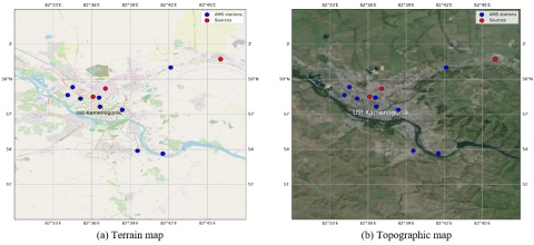
To calculate the sources of the spread of the harmful substance CO, three production and industrial facilities were considered - the Metallurgical Complex of Kazzinc LLP, Sogrinskaya CHP, Ust-Kamenogorsk CHP (Figure 1).
Air pollution data is received every 20 minutes from AMS. This data is transmitted online and securely stored on a server hosted in the Data Center of Akademset LLP. The data obtained is available in CSV format for analysis or use.
Chemical compounds CO, SO2 and NO2 were selected to carry out a computational experiment on the spread of pollutants. These substances are considered as the most dangerous for the environment, and on the other hand, their concentrations are regularly recorded by AMS for the city of Ust-Kamenogorsk.
The value of stoichiometric coefficients was assumed as in [32].
For the differential equation of the chemical substance $\mathrm{CO}$, the value of stoichiometric coefficients was taken as: $k_{60}=$ $5,1 * 10^{-5}, k_{65}=2,2 * 10^{-13}, k_{141}=4,3 * 10^{-15}$.
Similarly, for differential equations describing the propagation of chemicals SO2 and NO2, the corresponding stoichiometric coefficients were taken into account:
$\text{For}\quad\mathrm{SO}_2:=1 * 10^{-16}, k_{93}=2 * 10^{-17}, k_{115}=1,75 * 10^{-14}, k_{116}=1,75 * 10^{-14}, k_{139}=2,6 * 10^{-15}, k_{137}=1,4 * 10^{-5}$, $k_{140}=1,7 * 10^{-12}, k_{147}=6,3 * 10^{-14}, k_{148}=1 * 10^{-22}, k_{149}=1,5 * 10^{-12}, k_{150}=1 * 10^{-18}, k_{151}=1 * 10^{-20}, k_{152}=1 *$ $10^{-17}, k_{62}=6 * 10^{-16}$
$\text{For}\quad \mathrm{NO}_2: k_7=3 * 10^{-11}, k_{24}=1,8 * 10^{-14}, k_{26}=8,1 * 10^{-12}, k_{32}=1,9 * 10^{-11}, k_{51}=7 * 10^{-12}, k_{70}=8,8 * 10^{-12}$, $k_{72}=8,7 * 10^{-12}, k_{91}=1,4 * 10^{-12}, k_{117}=1,75 * 10^{-14}, k_{126}=8,1 * 10^{-12}, k_{130}=8,1 * 10^{-12}, k_{136}=7,6 * 10^{-12}, k_{10}=$ $1 * 10^{-11}, k_{32}=1,9 * 10^{-11}, k_{33}=2,1 * 10^{-1}, k_{36}=7,5 * 10^{-15}, k_{37}=2,6 * 10^{-15}, k_{43}=7,8 * 10^{-7}, k_{151}=1 * 10^{-20}$, $k_{155}=4,3 * 10^{-12}, k_8=2,25 * 10^{-11}, k_9=9,3 * 10^{-12}, k_{27}=7,8 * 10^{-3}, k_{28}=2,4 * 10^{-11}, k_{29}=2,9 * 10^{-17}, k_{36}=7,5 *$ $10^{-15}, k_{145}=1,4 * 10^{-11}$.
Figure 1(a) and (b) show the locations of the AMS stations and the sources of emissions in the city Ust-Kamenogorsk in a geographical coordinate system.
Figure 1. Location of AMS and pollution sources for pollutant CO
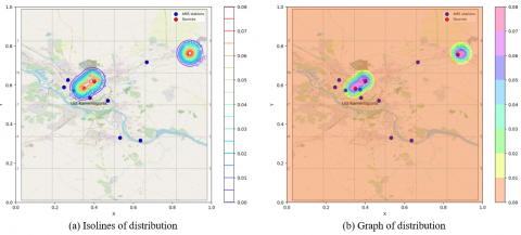
Figure 2. Distribution of pollution from three sources of emissions for pollutant CO in the case when speed components are 5 m/s
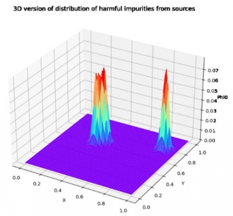
Figure 3. 3D version of distribution of pollution from three sources of emissions
Figure 2(a), (b) and Figure 3 show the distribution of the pollutant CO from three sources. According to the figures, the step-by-step distribution of the concentration of the pollutant CO can be seen in the atmosphere of the city of Ust-Kamenogorsk from three sources. It can be seen from the graphs that the pollutant is distributed from sources depending on the characteristics of atmospheric conditions, traffic flows, as well as the topography of the area. This visualizes the dynamics of pollution distribution in the environment and helps to identify the areas with the highest concentration of the substance.
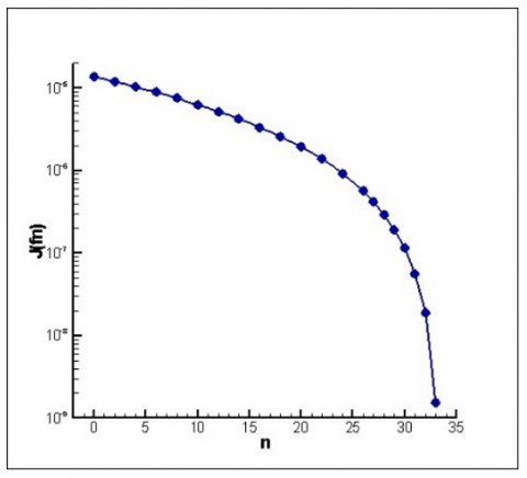
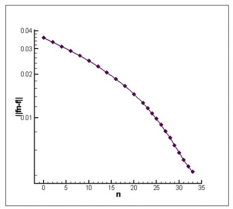
Numerical results of the inverse problem of source restoration demonstrate convergence to an exact solution. Based on the data presented in Figure 4, it can be argued that the value of the functional decreases to the level of $10^{-9}$ after 33 iterations. Analyzing Figure 5, we notice that the norm of the difference between the exact and reconstructed functions decreases to a value less than $10^{-2}$, which indicates that a minimum has been reached.
Figure 4. Graph of the functional $L\left(f^n\right)$
Figure 5. The norm of the difference between the exact function and the reconstructed function $\left\|f-f^n\right\|$
There are a number of models that allow you to simulate the spread of pollutants in the atmosphere, such as Box Models, Gaussian Models, Eulerian Model, Lagrangian Model, CFD Models, Aerosol Dynamic Models [34-37]. Some of them have disadvantages: they are stationary, do not take into account photochemistry and transformation of impurities, require large computing resources, etc.
The model considered in this paper offers a comprehensive solution combining the advantages of various methods and integrating technologies for more accurate and effective forecasting of air quality and atmospheric processes, such as accounting for the formation and transformation of harmful chemicals, data assimilation, wind direction, while spending less time for calculation.
This model allows you to identify the most vulnerable areas of an industrial city to improve air quality. By clarifying the concentration and volume of emissions from point sources, it will be possible to more accurately assess the risks to the urban environment. And also to offer recommendations to industrial enterprises, traffic management organizations, thermal power plants, the Department of Environmental Protection and local executive bodies to reduce the concentration of harmful impurities [7].
This work is part of a research project aimed at creating a geographic information system (GIS) for environmental monitoring. This model is integrated into the GIS system and the results of the model will be displayed on the developed information and analytical platform.
In the future, this model can be adapted for other industrial cities, as well as additional information, it will be possible to consider not only the data of the monitoring station, but also mobile sensors and remote sensing data. It is planned to consider other methods for solving this model, which will allow you to get a better result in less iteration and computing resources.
A review of the literature devoted to the study of tasks for the restoration of sources of atmospheric air pollution has been conducted.
The formulation of the problem of transport of pollutants is formulated taking into account photochemical transformations. An algorithm for solving the inverse problem is mathematically justified to clarify incomplete and inaccurate data from pollution sources.
It is shown that this algorithm allows to obtain a more accurate and complete picture of the concentration of pollutants in the atmospheric air of the city, since the mathematical model takes into account meteorological parameters and data from pollution sources. The developed algorithm corrects the data of pollution sources based on the AMS readings.
To illustrate the possibilities of the proposed method, the created software application implementing the method was used to simulate the transport of pollutants in the atmospheric air of the industrial city of Ust-Kamenogorsk. Incomplete and inaccurate data on emissions from industrial enterprises are clarified through the data observed by AMS.
The inclusion of impurities and photochemical reactions characteristic of the city in the transformation model complements the idea of the impact of industrial facilities on air quality. The results obtained are of great practical importance for the development of effective strategies in the field of regional environmental policy and provide a complete picture of the air conditions of industrial cities.
This research is funded by the Science Committee of the Ministry of Higher Education and Science of the Republic of Kazakhstan (grant No. BR18574148 "Development of geoinformation systems and monitoring of environmental objects").
|
GEMM |
Global Exposure Mortality Model |
|
TSP |
Total suspended particles |
|
MASINGAR |
Model of aerosol species in the global atmosphere |
|
AMS |
Automated monitoring stations |
|
CHP |
Combined Heat and Power |
|
CSV |
Comma-Separated Values |
|
CFD Models |
Computational Fluid Dynamics Models |
|
GIS |
Geographic information system |
[1] Assanov, D., Zapasnyi, V., Kerimray, A. (2021). Air quality and industrial emissions in the cities of Kazakhstan. Atmosphere, 12(3): 314. https://doi.org/10.3390/atmos12030314
[2] Kenessary, D., Kenessary, A., Adilgireiuly, Z., Akzholova, N., Erzhanova, A., Dosmukhametov, A., Syzdykov, D., Masoud, A.R., Saliev, T. (2019). Air pollution in kazakhstan and its health risk assessment. Ann Glob Health, 85(1): 133. https://doi.org/10.5334/aogh.2535
[3] Kerimray, A., Assanov, D., Kenessov, B., Karaca, F. (2020). Trends and health impacts of major urban air pollutants in Kazakhstan. Journal of the Air & Waste Management Association, 70(11): 1148-1164. https://doi.org/10.1080/10962247.(2020).1813837
[4] Assanov, D., Radelyuk, I., Perederiy, O., Galkin, S., Maratova, G., Zapasnyi, V., Klemeš, J.J. (2022). spatiotemporal patterns of air pollution in an industrialised city—A case study of ust-kamenogorsk, kazakhstan. Atmosphere, 13(12): 1956. https://doi.org/10.3390/atmos13121956
[5] Kerimray, A., Azbanbayev, E., Kenessov, B., Plotitsyn, Alimbayeva, D., Karaca, F. (2020). Spatiotemporal variations and contributing factors of air pollutants in Almaty, Kazakhstan. Aerosol and Air Quality Research, 20(6): 1340-1352. https://doi.org/10.4209/aaqr.2019.09.0464
[6] Temirbekov, N., Kasenov, S., Berkinbayev, G., Temirbekov, A., Tamabay, D., Temirbekova, M. (2023). Analysis of data on air pollutants in the city by machine-intelligent methods considering climatic and geographical features. Atmosphere, 14(5): 892. https://doi.org/10.3390/atmos14050892
[7] Temirbekov, N., Temirbekova, M., Tamabay, D., Kasenov, S., Askarov, S., Tukenova, Z. (2023). Assessment of the negative impact of urban air pollution on population health using machine learning method. International Journal of Environmental Research and Public Health, 20(18): 6770. https://doi.org/10.3390/ijerph(2018)6770
[8] Madiyarov, M., Temirbekov, N., Alimbekova, N., Malgazhdarov, Y., Yergaliyev, Y. (2023). A combined approach for predicting the distribution of harmful substances in the atmosphere based on parameter estimation and machine learning algorithms. Computation, 11(12): 249. https://doi.org/10.3390/computation11120249
[9] Baimatova, N., Koziel, J.A., Kenessov, B. (2015). Quantification of benzene, toluene, ethylbenzene and o-xylene in internal combustion engine exhaust with time-weighted average solid phase microextraction and gas chromatography mass spectrometry. Analytica Chimica Acta, 873: 38-50. https://doi.org/10.1016/j.aca.2015.02.062
[10] Temirbekov, N., Malgazhdarov, Y., Tamabay, D., Temirbekov, A. (2023). Atmospheric modelling of photochemical transformations of pollutants: Impact of weather conditions and diurnal cycle (Case study: Ust-Kamenogorsk, Kazakhstan). Mathematical Modelling of Engineering Problems, 10(5): 1699-1705. https://doi.org/10.18280/mme100520
[11] Temirbekov, N., Malgazhdarov, Y., Tamabay, D., Temirbekov, A., (2023). Mathematical and computer modeling of atmospheric air pollutants transformation with input data refinement. Indonesian Journal of Electrical Engineering and Computer Science, 32(3): 1405-1416. http://doi.org/10.11591/ijeecs.v32.i3.pp1405-1416
[12] Lukyanets, A., Gura, D., Savinova, O., Kondratenko, L. Lushkov, R. (2023). Industrial emissions effect into atmospheric air quality: Mathematical modelling. Reviews on Environmental Health, 38(2): 385-393. https://doi.org/10.1515/reveh-2022-0005
[13] Berlyand, M.E. (1985). Forecast and Regulation of Atmospheric Pollution. Boston, Kluwer Academic Publishers.
[14] Marchuk, G.I. (2023). Mathematical modeling in the problem of the environment, M.: Nauka, 320: 1982. http://www.prometeus.nsc.ru/science/schools/marchuk/biblio/cont1982.ssi.
[15] Marchuk G.I. (1975). Methods of Numerical Mathematics. New York: Springer-Verlag.
[16] Sasaki, Y. (1955). A fundamental study of the numerical prediction based on the variational principle. Journal of the Meteorological Society of Japan, 33(6): 262-275. https://doi.org/10.2151/jmsj1923.33.6_262
[17] Penenko V.V. (1981). Methods of Numerical Modeling of Atmospheric Processes, Leningrad: Gidrometeoizdat. https://www.libex.ru/detail/book849287.html, accessed on Jan. 29, 2024.
[18] Dimet, F.X.L., Talagrand, O. (1986). Variational algorithms for analysis and assimilation of meteorological observations: theoretical aspects. Tellus. Series A, Dynamic meteorology and oceanography, 38A(2): 97-110. https://doi.org/10.3402/tellusa.v38i2.11706
[19] Yu, L., Malanotte-Rezzoli, P. (1998). Inverse modeling of seasonal variations in the North Atlantic Ocean. Journal of Physical Oceanography, 28(5): 902-922. https://doi.org/10.1175/1520-0485(1998)028<0902:IMOSVI>2.0.CO;2
[20] Marchuk, G.I., Aloyan, A.E., Arutyunyan, V.O. (2005). Adjoint equations and transboundary transport of pollutants. Ekologicheskiy Vestnik Nauchnogo Tsentra ChES, 2: 54-64.
[21] Aloyan, A.E., Arutyunyan, V.O. (2007). Control theory and environmental risk assessment. Air, Water and Soil Quality Modelling for Risk and Impact Assessment, 45-54. https://doi.org/10.1007/978-1-4020-5877-6_4
[22] Yu, A., Kriksin, S.N., Plushev, E.A., Samarskaya, et al., (1995). The inverse problem of restoring the source density for the convection-diffusion equation. Mathematical Modelling, 7(11): 95-108.
[23] Kochergin, V. (2009). Using conjugate equations to solve environmental problems, environmental safety of coastal and shelf zones and integrated use of shelf resources. Scientific Electronic Library, 18: 93-99. https://elibrary.ru/download/elibrary_29078365_30715768.pdf, accessed on Jun. 3, 2024.
[24] Panasenko, E.A., Starchenko, A.V. (2008). Numerical solution of some inverse problems with various types of sources of atmospheric pollution. Vestnik Tomskogo Gosudarstvennogo Universiteta. Matematika i Mekhanika, 2(3): 47-55.
[25] Kochergin, S.V., Kochergin, V.S. (2016). Realization of variational algorithm at identification of input parameters of model of transfer of passive impurity in Azov Sea. Environmental Safety of Coastal and Offshore Zones of the Sea, 3: 50-58. https://vestnik.kubsu.ru/article/view/701/1197, accessed on Jun. 3, 2024.
[26] Penenko, A.V., Konopleva, V.S., Penenko, V.V. (2022). Inverse modeling of atmospheric chemistry with a different evolution solver: Inverse problem and Data assimilation. IOP Conference Series: Earth and Environmental Science, 1023(1): 012015. https://doi.org/10.1088/1755-1315/1023/1/012015
[27] Aloyan, A.E., Arutyunyan, V.O., Haymet, A.D., He, J.W., Kuznetsov, Y.A., Lubertino, G. (2003). Modeling of air quality in the Houston-Galveston-Brazoria area. Environment International, 29(2-3): 377-383.
[28] Onishi, K., Sekiyama, T.T., Nojima, M., Kurosaki, Y., Fujitani, Y., Otani, S., Maki, T., Shinoda, M., Kurozawa, Y., Yamagata, Z. (2018). Prediction of health effects of cross-border atmospheric pollutants using an aerosol forecast model. Environment International, 117: 48-56. https://doi.org/10.1016/j.envint.2018.04.035
[29] Oxley, T., Dore, A., ApSimon, H., Hall, J.R., Kryza, M. (2013). Modelling future impacts of air pollution using the multi-scale UK Integrated Assessment Model (UKIAM). Environment International, 61: 17-35. https://doi.org/10.1016/j.envint.2013.09.009
[30] Tong, D.Q., Gill, T.E., Sprigg, W.A., et al. (2023). Health and safety effects of airborne soil dust in the americas and beyond. Reviews of Geophysics, 61(2): e(2021)RG000763. https://doi.org/10.1029/2021RG000763
[31] Kulmala, M., Kokkonen, T., Ezhova, E., Baklanov, A., Mahura, A., Mammarella, I., Bäck, J., Lappalainen, H.K., Tyuryakov, S., Kerminen, V.M., Zilitinkevich, S., Petäjä, T. (2023). Aerosols, clusters, greenhouse gases, trace gases and boundary-layer dynamics: on feedbacks and interactions. Boundary-Layer Meteorology, 186: 475-503. https://doi.org/10.1007/s10546-022-00769-8
[32] Danaev, N.T. Temirbekov, A.N., Malgazhdarov, E.A. (2014). Modeling of pollutants in the atmosphere based on photochemical reactions. Eurasian Chemico-Technological Journal, 16(1): 61-71. https://doi.org/10.18321/ectj170
[33] Environmental statistics. (2023). Bureau of national statistics of the agency for strategic planning and reforms of the Republic of Kazakhstan. https://stat.gov.kz/ru/industries/environment/stat-eco/, accessed on Jan. 23, 2024.
[34] Pengpom, N., Vongpradubchai, S., Rattanadecho, P. (2019). Numerical study of a combined pollutant concentration dispersion and convective heat transfer in a two-dimensional factory model. International Journal of Heat and Technology, 37(2): 649-658. https://doi.org/10.18280/ijht.370237
[35] Modi, M., Venkata, R.P., SK, L.A., Hussain, Z. (2013). A review on theoretical air pollutants dispersion models. International Journal of Pharmaceutical, Chemical & Biological Sciences, 3(4): 1224-1230.
[36] Lotrecchiano, N., Sofia, D., Giuliano, A., Barletta, D., Poletto, M. (2020). Pollution dispersion from a fire using a Gaussian plume model. International Journal of Safety and Security Engineering, 10(4): 431-439. https://doi.org/10.18280/ijsse.100401
[37] Sharma, N., Chaudhry, K.K., Rao, C.V.C. (2004). Vehicular pollution prediction modelling: A review of highway dispersion models. Transport Reviews, 24(4): 409-435. https://doi.org/10.1080/0144164042000196071