Moses O. Petinrin | Al-Amin Owodunni | Rasaq A. Kazeem | Omolayo M. Ikumapayi* | Sunday A. Afolalu | Esther T. Akinlabi
© 2022 IIETA. This article is published by IIETA and is licensed under the CC BY 4.0 license (http://creativecommons.org/licenses/by/4.0/).
OPEN ACCESS
In this paper, the temperature distribution in a slab was investigated. A model based on the Boltzmann transport equation without heat source was simplified using the Bhatnagar-Gross-Krook (BGK) approximation was applied. This is an example of the Lattice Boltzmann Method. The model was developed based on using a D2Q4 lattice arrangement for the medium of study. To obtain results, the model was tested on different cases: Two box-shaped slabs with different boundary conditions, and a T-shaped and an L-shaped slabs to determine the temperature distributions different times t > 0. The results obtained based on the developed model were validated with the enterprise software COMSOL Multiphysics which is based on the Finite Element Method. For the two cases of box-shaped and the T-shaped slabs, their results were in nearly perfect agreement with the finite element method. However, for the L-shaped slab, there was good agreement at most points apart from the regions where there was change of shape. In conclusion there is high agreement between the results of LBM and using COMSOL, which proves that LBM can be used to determine temperature distribution in a slab accurately.
lattice Boltzmann, temperature distribution, slab, model, COMSOL multiphysics, finite element method
Heat transfer across different materials is a common occurrence in traditional sciences and engineering, such as in the cooling of turbine blades, heat exchangers, and electronic devices and the transfer of heat between solids and the fluids that surround them [1]. A configuration that is frequently observed in engineering components and systems is a solid slab that exists having its ends at different temperatures. Heat energy is transferred across the ends of the slab by thermal conduction [2].
CFD techniques are powerful instruments for exploring physical and chemical processes, as well as solving thermal, fluid, and other real-world engineering issues. The finite difference method (FDM), finite element method (FEM), and finite volume method (FVM) are all common CFD techniques [3]. Using nodal values, the finite difference technique provides an estimated solution. From a succession of local approximations of solutions derived from local data, the finite element technique produces an approximate global solution [4]. The final volume technique calculates an estimated solution by averaging the solution's average value across a certain volume.
In applying the lattice Boltzmann method (LBM) the behaviour of a group of particles is studied as a whole and a distribution function is created to express the properties of the collection of particles. LBM offers several advantages. Its calculation technique is easier since its foundation is the Lattice Boltzmann equation, whose solution is simpler than the Navier-Stokes equation, which is the foundation of the finite volume method. LBM can take full use of parallel computing, which divides huge problems into smaller ones that can be tackled at the same time. This cuts down on the time it takes to find a solution. LBM stands for high computing performance in terms of solution correctness and stability [5].
The LBM can be used in a variety of problems concerning the flow of fluids and heat, especially those that involve conduction, convection, and radiation. Wolf-Gladrow [6] is one of the pioneering researchers to establish an LB formula for problems relating to diffusion, he demonstrated how simple it is to derive such a model from the kinetic equation. Ho et al. [7] employed the LBM to investigate the behaviour of conduction of heat in a non-Fourier problem in a plane medium. The heat transfer together with the transmission–reflection phenomenon is numerically investigated when heat passes through a joint interface of construction with a double layer. Miller and Succi [8] developed a LB model which studies anisotropic crystal growth in melt with improved computation power. A linear collision matrix on a face-centred hyper-cubic lattice is used to manage hydrodynamics and heat transport.
Semma et al. [9] applied LBM in modelling the relationships between convective flows and the liquid/solid interfaces in rectangular cavities. It employed the customised probabilistic bounce-back approach. This novel methodology is found to be a useful method for problems with moving boundaries. To simulate thermo-hydrodynamics, Chatterjee [10] developed a thermal LB algorithm whose foundation is the complete enthalpy formulation because it is based on kinetic theory and thermodynamic basics.
An LB approach that studied convection under the influence of natural forces in the fluid with porous sections and whose viscosity is temperature-dependent was proposed by Guo and Zhao [11]. Mishra et al. [12] developed a basic LBM to solve the energy equation. Zhao et al. [13] developed the LBM algorithm for solving problems during the process of conducting heat in three-dimensional porous media to explore the conduction problem existing inside a porous wick.
Shafeie et al. [14] studied the performance of heat transfer for single-phase heat sinks with the structure of micro pin-fin, which is another example of numerical analysis in a heat transfer problem. Eshraghi and Felicelli [15] created a model that uses LBM to handle phase change heat conduction difficulties. It was discovered that phase transition happens over a wide temperature range rather than at a single temperature. LBM was utilised by Semma et al. [16] to handle problems related to melting and solidification Heat transfer due to the movement of the fluid in the molten zone has been found to have a considerable impact on the rate at which a cavity heated from the bottom is melted.
Chen et al. [17] introduced LBM for conjugate heat research, which is defined as the mixing of conduction and convection in a fluid flowing over a solid. The results of the model and the data were in good accord. Chaabane et al. [9] solved energy equation for a two dimensional enclosure problem with several boundary conditions using the LBM, their results were also found to be in good agreement with that of finite volume method. Lu et al. [18] suggested a thermal LB equation to predict heat transfer in their paper. Gao et al. [19] suggested a modified LBM for conjugate heat transport in porous medium systems. Previous research's analytical and numerical solutions correspond well with the model.
Seddiq et al. [20] applied the Lattice Boltzmann Equation to create a model for heat transmission at the fluid-solid boundary. The location that was discovered to possess the highest rate of heat transfer does not affect the thermal characteristics of the fluid and solid mediums, according to the study. For transfer of heat involving a change of state such as solidification and melting, Su and Davidson [21] built a model on a time step adjustable non-dimensional LBM.
In this work, two-dimensional temperature distribution patterns within slabs of three different shapes and boundary conditions are predicted using the lattice Boltzmann method. The slabs are of two box-shaped (rectangular) and a T-shaped and an L-shaped, which are deviations from the common shapes in the available literature. The developed model is validated with the results of the models developed with finite element based computational code, COMSOL Multiphysics to ensure the accuracy of the predictions.
2.1 The heat diffusion equation
In this study, the lattice Boltzmann method has been used to solve a heat diffusion problem. The heat diffusion equation for a two-dimensional study is presented in Eq. (1).
$\rho C \frac{\partial T}{\partial t}=\frac{\partial}{\partial x}\left(k \frac{\partial T}{\partial x}\right)+\frac{\partial}{\partial y}\left(k \frac{\partial T}{\partial y}\right)$ (1)
T denotes temperature, C denotes medium's specific heat, ρ denotes density, and k denotes thermal conductivity. The thermal conductivity (k), density (ρ), and specific heat diffusion (C) influence the heat diffusion caused by molecular action. For a case with constant thermal conductivity, the previous equation appears in the form of Eq. (2):
$\frac{\partial T}{\partial t}=\alpha\left(\frac{\partial^2 T}{\partial x^2}+\frac{\partial^2 T}{\partial y^2}\right)$ (2)
where, α denotes thermal diffusivity (k/ρC). As a result, the thermal diffusivity which is a material property is the parameter that determines heat diffusion. The rate of the diffusion process increases as α increases.
2.2 The lattice Boltzmann method
For the temperature distribution function, the kinetic equation is stated as depicted in Eq. (3) [22]:
$\frac{\partial f_k(x, t)}{\partial t}+c_k \cdot \frac{\partial f_k(x, t)}{\partial x}=\Omega_k$ (3)
where, k = 1,2 for (one dimensional problems, D1Q2).
The streaming process is represented by the variables on the left side of equation 3, in which the distribution function flows with velocity along the lattice linkages is presented in Eq. (4).
$c_k=\frac{\Delta x}{\Delta t}$ (4)
The variable on the right side k in equation 3 is called the collision operator. It denotes the distribution function's fk rate of change during the collision process. Ωk can be replaced by the BGKW approximation for the collision operator, and this will give Eq. (5):
$\Omega_k=-\frac{1}{\tau}\left[f_k(x, t)-f_k^{e q}(x, t)\right]$ (5)
where, τ denotes the relaxation time.
The kinetic equation with BGK approximation can be written in a discrete form as indicated in Eq. (6).
$\frac{f_k(x+\Delta x, t+\Delta t)-f_k(x, t)}{\Delta t}+$$c_k \cdot \frac{f_k(x+\Delta x, t+\Delta t)-f_k(x, t+\Delta t)}{\Delta x}$$=-\frac{1}{\tau}\left[f_k(x, t)-f_k^{e q}(x, t)\right]$ (6)
from Eq. (4) $\Delta x=c_k \Delta t$ substituting in Eq. (6), is replaced with Eq. (7):
$f_k(x+\Delta x, t+\Delta t)-f_k(x, t)=$$-\frac{\Delta t}{\tau}\left[f_k(x, t)-f_k^{e q}(x, t)\right]$ (7)
Eq. (7) is the main equation that does all the work in solving diffusion problems in one-dimensional domains, it is shortened to produce Eq. (8).
$f_k(x+\Delta x, t+\Delta t)=f_k(x, t)[1-\omega]+\omega f_k^{e q}(x, t)$ (8)
2.3 Two-dimensional LBM equation
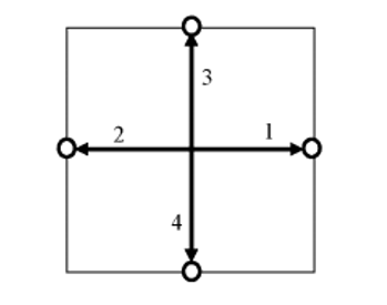
However, the subject of this paper is in solving two-dimensional diffusion problems and the D2Q4 lattice arrangement is employed for this research work (see Figure 1). The Kinetic Lattice Boltzmann equation has two steps: Collision and streaming. The collision step without including a force function is represented in Eq. (9):
$f_k(x, y, t+\Delta t)=$$f_k(x, y, t)[1-\omega]+\omega f_k^{e q}(x, y, t)$ (9)
where, k = 1 – 4.
Then, the streaming step is written as in the form of Eq. (10):
$f_k(x+\Delta x, y+\Delta y, t+\Delta t)=f_k(x, y, t+\Delta t)$ (10)
where, k = 1 – 4.
For example, in the streaming step f1 (i, j) streams to f1 (i + 1, j), f2 (i, j) streams to f2 (i - 1, j), f3 (i, j) streams to f3 (i, j + 1) and f4 (i, j) streams to f4 (i, j - 1). The weighting factor and the thermal diffusivity.
Figure 1. D2Q4 lattice arrangement
The weighting factor:
$\omega_i=\left\{\frac{1}{4}\right\}$ for i = 1, 2, 3, 4 (11)
Also thermal diffusivity:
$\alpha=\frac{\Delta x^2}{2 \Delta t}\left(\frac{1}{\omega}-\frac{1}{2}\right)$ (12)
2.4 Boundary conditions
The LBE has its basis in particle distributions functions, and thus the macroscopic hydrodynamic quantities' boundary conditions must be translated to particle distributions' boundary conditions.
2.5 Dirichlet boundary condition
In thermodynamics, Dirichlet boundary conditions consist of boundaries held at fixed temperatures. Considering a case where the boundaries temperature fixed for the bottom and left borders are known.
T = C1 at x = 0 and T = C2 at y = 0.
$f_1+f_2+f_3+f_4=T$ (13)
f2 and f4 can be solved for using the streaming step:
$f_2(i, j)=f_2(i+1, j)$ and $f_4(i, j)=f_4(i, j+1)$ (14)
f1 and f3 can be solved by using the equation for flux conservation:
$f_1^{e q}-f_1+f_2^{e q}-f_2=0$ (15)
ω = 0.25 at every streaming direction.
$f_1^{e q}=f_2^{e q}=0.25 \mathrm{Cl}$ (16)
Therefore:
$f_1=0.5 C_1-f_2$ (17)
Similarly:
$f_3=0.5 C_2-f_4$ (18)
If temperature T is fixed on the right and top borders, then f2 and f4 respectively need to be calculated.
2.6 Constant heat flux
As expressed in Eq. (19), the constant heat flow is presented as defined in [23]:
$k \frac{\partial T}{\partial x}=q$ (19)
The boundary condition above will be approximated using the finite difference approach to become:
$k \frac{T(i+1, j)-T(i, j)}{\Delta x}=q$ (20)
This is re-written as:
$T(i, j)=T(i+1, j)-\frac{q \Delta x}{k}$ (21)
$f_1(i, j)=f_1(i+1, j)-\frac{q \Delta x}{k}$ (22)
2.7 Adiabatic boundary condition
For example:
$\frac{\partial T}{\partial x}=0$ (23)
The boundary condition above is approximated using a finite difference approach to become:
$\frac{T(i+1, j)-T(i, j)}{\Delta x}=0$ (24)
This is rewritten as $T(i, j)=T(i+1, j)$. Therefore:
$f_1(i, j)+f_2(i, j)+f_3(i, j)+f_4(i, j)=f_1(i+1, j)+f_2(i+1, j)+f_3(i+1, j)+f_4(i+1, j)$ (25)
2.8 Methodology flow chart
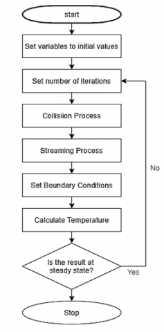
The steps by step processes in performing a simulation using LBM are shown in Figure 2.
Figure 2. Methodology flow chart
Case 1
Different boundary conditions are applied to a two-dimensional box-shaped slab as seen in Figure 3. The slab was initially at a non-dimensional temperature of 0.0. For times greater than 0, the vertical border at the origin is exposed to a relatively high temperature of a non-dimensionalized quantity of 1.0, while the other boundaries remain unchanged. The domain has a length of 100 units. Evaluate the distribution of temperature in the slab at various time periods. Compare the findings from the LB and FE approaches. The horizontal and vertical lengths are 100 units, and the thermal diffusivity is 0.25.
Figure 3. Case 1: Box-shaped slab
Result
The temperature distributions along line y = 50 obtained by the LBM algorithm and by the FEM algorithm were plotted and shown in Figure 4.
Figure 4. Temperature distribution in box-shaped slab at different time intervals for y = 50 units
It can be observed that there is a strong agreement between the lattice Boltzmann result and the result generated using the finite element method for all time steps in the study. Also, the plot at 6000 s shows the maximum limit for the temperature distribution in the domain, which is when the domain is at a steady state.
Case 2
For the problem in case 1, evaluate the temperature distribution at different positions as shown in Figure 5 for a time step of 24000 units.
Figure 5. Case 2: Box-shaped slab
Result
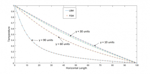
The temperature distributions along line y = 10, 30, 60, and 90 obtained by the LBM and by the FEM were plotted and shown in Figure 6.
Figure 6. Temperature distribution in box-shaped slab at different vertical distances
It can be observed that there is strong agreement between the temperature distribution generated with LBM and the FEM. However, there are some inconsistencies around the region where the shape changes.
Case 3
Different boundary conditions are applied to a two-dimensional T shaped slab as seen in Figure 7. The slab was initially at a temperature of 0.0. For times greater than 0, the vertical border at the origin is exposed to a relatively high temperature of a non dimensionalized quantity of 1.0, while the other boundaries remain unchanged. The domain has a length of 100 units. Evaluate the distribution of temperature in the slab at various time periods. Compare the findings from the LB and FE approaches. The horizontal and vertical lengths are 100 units, given that the thermal diffusivity of the medium is 0.25.
Figure 7. T-shaped slab
Result
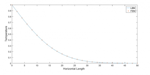
Figure 8. Temperature distribution in T-shaped slab at y = 50 units
The temperature distributions along line y = 50 obtained b LBM and by FEM were plotted and shown in Figure 8. It can be observed that there is good agreement between the temperature distribution generated with LBM and the FEM.
Case 4
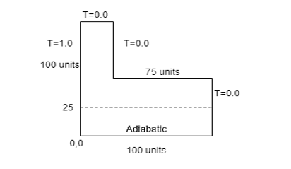
Different boundary conditions are applied to a two-dimensional L-shaped slab as seen in Figure 9. The slab was initially at a non-dimensional temperature of 0.0. For times greater than 0, the vertical border at the origin is exposed to a relatively high temperature of a non dimensionalized quantity of 1.0, while the other boundaries remain unchanged. The domain has a length of 100 units. Evaluate the distribution of temperature in the slab at various time periods. Compare the findings from the LB and FE approaches. The horizontal and vertical lengths are 100 units, given that the thermal diffusivity of the medium is 0.25.
Figure 9. L-shaped slab
Result
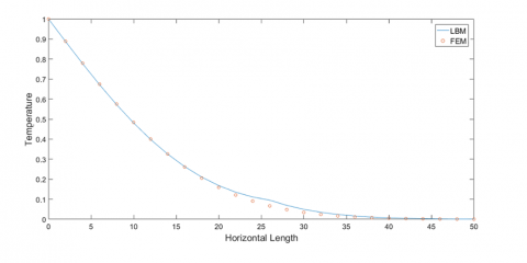
Figure 10. Temperature distribution in L-shaped slab at y = 25 units
It can be observed that there is an agreement between the temperature distribution generated with LBM and the FEM (Figure 10). However, there are some inconsistencies around the region where the shape changes.
The research has been able to achieve the development of a mathematical model based on the Boltzmann transport equation to investigate temperature distribution in a slab of various shapes. The model developed was tested by using different shapes of slabs and boundary conditions. The results obtained for the temperature distribution using LBM were in good agreement with the result obtained using FEM with the COMSOL Multiphysics software. This implies that the Lattice Boltzmann model can be used as an alternate method for the proprietary software.
|
LBM |
lattice boltzmann method |
|
FEM |
finite element method |
|
CFD |
computational fluid dynamics |
|
f |
particle distribution function |
|
m |
mass of particle |
|
t |
time of particle |
|
v |
velocity of particle |
|
x,y |
Position |
|
ci |
lattice velocity |
|
feq |
equilibrium distribution function |
|
F |
force acting on the particle of |
|
C |
specific heat |
|
q |
heat flux |
|
Greek symbols |
|
|
Ω |
collision operator |
|
ω |
weighting factor |
|
α |
thermal diffusivity |
|
k |
thermal conductivity |
|
ρ |
Density |
|
τ |
relaxation time |
[1] Korba, D., Li, L. (2020). Interface treatment for conjugate conditions in the Lattice Boltzmann method for the convection diffusion equation. Computational Fluid Dynamics Simulations. https://doi.org/10.5772/intechopen.86252
[2] Cheng, C.H., Yu, J.H. (1995). Conjugate heat transfer and buoyancy-driven secondary flow in the cooling channels within a vertical slab. Numerical Heat Transfer, Part A: Applications, 28(4): 443-460. https://doi.org/10.1080/10407789508913755
[3] Fatoba, O.S., Lasisi, A.M., Ikumapayi, O.M., Akinlabi, S.A., Akinlabi, E.T. (2021). Computational modelling of laser additive manufactured (LAM) Titanium alloy grade 5. Materialstoday: Proceedings, 44(1): 1254-1262. https://doi.org/10.1016/j.matpr.2020.11.262
[4] Ikumapayi, O.M., Atta, B.I., Afolabi, S.O., Adeoti, O.M., Bodunde, O.P., Akinlabi, S.A., Akinlabi, E.T. (2020). Numerical modelling and mechanical characterization of pure aluminium 1050 wire drawing for symmetric and axisymmetric plane deformations. Mathematical Modelling of Engineering Problems, 7(4): 539-548. https://doi.org/10.18280/mmep.070405
[5] Mondal, B., Mishra, S.C. (2007). Application of the lattice Boltzmann method and the discrete ordinates method for solving transient conduction and radiation heat transfer problems. Numerical Heat Transfer Applications, Part A: Applications, 52(8): 757-775. https://doi.org/10.1080/10407780701347663
[6] Wolf-Gladrow, D. (1995). A lattice Boltzmann equation for diffusion. Journal of Statistical Physics, 79: 5-6, 1023-1032. https://doi.org/10.1007/BF02181215
[7] Ho, J.R., Kuo, C.P., Jiaung, W.S. (2003). Study of heat transfer in multilayered structure within the framework of dual-phase-lag heat conduction model using lattice Boltzmann method. International Journal of Heat and Mass Transfer, 46(1): 55-69. https://doi.org/10.1016/S0017-9310(02)00260-0
[8] Miller, W., Succi, S. (2002). A lattice Boltzmann model for anisotropic crystal growth from melt. Journal of Statistical Physics, 107(1): 173-186. https://doi.org/10.1023/A:1014510704701
[9] Semma, E., El Ganaoui, M., Bennacer, R., Mohamad, A.A. (2008). Investigation of flows in solidification by using the lattice Boltzmann method. International Journal of Thermal Sciences, 47(3): 201-208. https://doi.org/10.1016/j.ijthermalsci.2007.02.010
[10] Chatterjee, D. (2009). An enthalpy-based thermal lattice Boltzmann model for non-isothermal systems. EPL (Europhysics Letters), 86(1): 14004. https://doi.org/10.1209/0295-5075/86/14004
[11] Guo, Z.L., Zhao, T.S. (2005). Lattice Boltzmann simulation of natural convection with viscosity in a porous cavity. Mechanical Engineering, 5(1/2): 110-117. http://dx.doi.org/10.1504/PCFD.2005.005823
[12] Mishra, S.C., Lankadasu, A., Beronov, K.N. (2005). Application of the lattice Boltzmann method for solving the energy equation of a 2-D transient conduction-radiation problem. International Journal of Heat and Mass Transfer, 48(17): 3648-3659. https://doi.org/10.1016/j.ijheatmasstransfer.2004.10.041
[13] Zhao, K., Li, Q., Xuan, Y.M. (2009). Investigation on the three-dimensional multiphase conjugate conduction problem inside porous wick with the lattice Boltzmann method. Science in China, Series E: Technological Sciences, 52(10): 2973-2980. https://doi.org/10.1007/s11431-009-0103-7
[14] Shafeie, H., Abouali, O., Jafarpur, K., Ahmadi, G. (2013). Numerical study of heat transfer performance of single-phase heat sinks with micro pin-fin structures. Applied Thermal Engineering, 58(1-2): 68-76. https://doi.org/10.1016/j.applthermaleng.2013.04.008
[15] Eshraghi, M., Felicelli, S.D. (2012). An implicit lattice Boltzmann model for heat conduction with phase change. International Journal of Heat and Mass Transfer, 55(9-10): 2420-2428. https ://doi.org/10.1016/j.ijheatmasstransfer.2012.01.018
[16] Chaabane, R., Askri, F., Nasrallah, S.B. (2010). Numerical modeling of boundary conditions for two dimansional conduction heat transfer equation using lattice boltzmann method. International Journal of Heat and Technology, 28(2): 53-59.
[17] Chen, S., Yan, Y.Y., Gong, W. (2017). A simple lattice Boltzmann model for conjugate heat transfer research. International Journal of Heat and Mass Transfer, 107: 862-870. https://doi.org/10.1016/j.ijheatmasstransfer.2016.10.120
[18] Lu, J.H., Lei, H.Y., Dai, C.S. (2018). A unified thermal lattice Boltzmann equation for conjugate heat transfer problem. International Journal of Heat and Mass Transfer, 126: 1275-1286. https://doi.org/10.1016/j.ijheatmasstransfer.2018.06.031
[19] Gao, D.Y., Chen, Z.Q., Chen, L.H., Zhang, D.L. (2017). A modified lattice Boltzmann model for conjugate heat transfer in porous media. International Journal of Heat and Mass Transfer, 105: 673-683. https://doi.org/10.1016/j.ijheatmasstransfer.2016.10.023
[20] Seddiq, M., Maerefat, M., Mirzaei, M. (2014). Modeling of heat transfer at the fluid-solid interface by lattice Boltzmann method. International Journal of Thermal Sciences, 75: 28-35. https://doi.org/10.1016/j.ijthermalsci.2013.07.014
[21] Su, Y., Davidson, J.H. (2016). A new mesoscopic scale timestep adjustable non-dimensional lattice Boltzmann method for melting and solidification heat transfer. International Journal of Heat and Mass Transfer, 92: 1106-1119. https://doi.org/10.1016/j.ijheatmasstransfer.2015.09.076
[22] Benabderrahmane, F., Draoui, B., Douha, M., Kaid, N., Merabti, A., Sahli, A., Moungar, H. (2020). The lattice Boltzmann method use to simulate natural convection in a single-chapel greenhouse. International Journal of Design & Nature and Ecodynamics, 15(4): 499-505. https://doi.org/10.18280/ijdne.150406.
[23] Salah, B., Nadia, M., Mohamed, L., Salem, M., Chutarat, T., Weerawat, S., Giulio, L., Hijaz, A., Younes, M. (2022). Investigation and Analysis of Soil Temperature under Solar Greenhouse Conditions in a SemiArid Region. International Journal of Design & Nature and Ecodynamics, 17(3): 325-332. https://doi.org/10.18280/ijdne.170301