Jian Yu | Hongbiao Gu* | Baoming Chi | Weifeng Shan | Mingyuan Wang
© 2020 IIETA. This article is published by IIETA and is licensed under the CC BY 4.0 license (http://creativecommons.org/licenses/by/4.0/).
OPEN ACCESS
Groundwater level in wells, i.e., well water level (WWL) is an important index in hydrological monitoring during earthquakes. Due to the complex dynamics of groundwater, the WWL might change under seismic actions. This paper attempts to identify the long-term correlation between WWL and earthquakes, and disclose the topological features of groundwater dynamics. Taking Nanxi Well as an example, the authors conducted state space analysis on the raw series and trend of WWL to eliminate interferences like barometric pressure, rainfall, and solid tide, creating the trend time series. Then, the raw series and trend time series were converted into the raw visible graph (VG) network and trend VG network, respectively. Further, the global period was divided into five local time windows, and the two VG networks were compared by global aspect, local aspect, and topological properties of complex networks. The results show that the nodes of high degrees are closely related to the seismic response of the WWL in Nanxi Well; all VG networks are scale free and hierarchical; the seismic response of the WWL in the well is reflected by degree correlation; the community division of raw VG network was basically the same as that of trend VG network. The research findings provide insights to the seismic response of WWL and the dynamic fluctuation of groundwater level.
groundwater, earthquake, visibility graph (VG), time series, state space
Earthquake is a dangerous natural disaster that releases a huge amount of energy from the earth’s crust in a short period. Despite the difficulty in earthquake prediction, seismologists have discovered some pre-seismic abnormalities that help to forecast earthquakes. The abrupt variation in groundwater level in wells, i.e., well water level (WWL), is one of these abnormal phenomena [1-3]. The WWL, which reflects the stress fluctuations in the well-aquifer system, has been successfully used to predict earthquakes [4]. The abnormal variation in the WWL can be captured through the research of co-seismic groundwater level. In fact, it is very meaningful to study the co-seismic WWL, for the seismic-induced variation in the WWL affects the groundwater supply [5], alters the chemical composition of water, and triggers eruption of mud volcanos [6] and even secondary earthquakes [7].
The existing studies on the seismic-induced variation in the WWL mainly focus on the variation mechanism. Most of them ascribe the variation to the static stress and seismic wave generated by the seismic energy. The static stress of earthquakes could consolidate the aquifer, and change the static pore strains, making the aquifer more fractured [8]. Meanwhile, the seismic wave might dredge or block the aquifer, regulate pore pressure, and intensify aquifer fracturing, thereby leading to permeability changes. The possible mechanism of seismic-induced variation in the WWL has been analyzed based on different earthquake magnitudes and epicentral distances. In near-field earthquakes, the variation occurs as the pore pressure changes with the static stress of large earthquakes, or as the seismic wave transforms the permeability; In intermediate- and far-field earthquakes, the variation is mainly the result of the permeability changes caused by seismic wave [9].
The variation of groundwater level is a complex issue. Apart from earthquakes, the WWL could be affected by nontectonic factors like barometric pressure, precipitation, solid tide, and human activities. To pinpoint seismic signals, some scholars have separated the response of barometric pressure, rainfall, and solid tide from that of groundwater [10-13]. In addition, it is possible to acquire possible seismic signals, and even pre-seismic signals, from the groundwater. However, there is little report on the features of seismic-induced WWL variation from the perspective of system dynamics. Therefore, this paper aims to develop a new method to measure the seismic-induced WWL variation.
Complex network analysis has been widely used in many fields. This statistical tool describes the elements and relations of the target system as nodes and edges. After all, the dynamic change of every complex network is reflected by its specific topological features. In recent years, Lacasa et al. [14] proposed the visibility graph (VG) complex network analysis, which maps each time series into a complex network, and obtains the properties of the network through time series analysis. Since then, this analysis approach has been implemented in various fields, such as finance [15-20], heart rate monitoring [21, 22], oceanic tide, and earthquakes. For instance, Telesca et al. [23] analyzed the time series of oceanic tide level, and summed up the laws of degree distribution of the series: the range degree k<20 is related to local tide effects, and the range degree k>100 is related to global tide effects. Aguilar-San Juan, and Guzman-Vargas [24] transformed earthquake magnitude series into VG networks, and obtained the properties for main-shocks by altering the observation window.
This paper provides a new research perspective to the features of seismic-induced WWL variation, and the topological properties of WWL time series. Specifically, the VG complex network analysis was adopted to convert the WWL time series into complex networks, investigate the relationship between the degrees of complex network, WWL time series, and earthquakes. Furthermore, the interference of rainfall, barometric pressure, and solid tide on the WWL time series were eliminated through state space analysis. With the aid of the trend time series, the processed data was built into a VG complex network. In different time windows, the authors analyzed the degree correlation series and WWL responses to multiple earthquakes, and investigated various properties of VG complex networks, namely, degree distribution, assortative mixing, hierarchy, and community structure.
2.1 Data description
Located near the Huaying Mountains fault zone, Nanxi well (N: 28.9ºN; E: 104.9º) is a seismic monitoring well in southwestern China’s Sichuan Province. The fault zone lies between the main body of Sichuan Basin and the East Sichuan barrier fold belt, and develops along the axis of Huaying Mountains anticline. Consisting of 2-3 main faults, it is one of the most important fault zones in Sichuan Basin.
With the total depth of 101.5m, Nanxi Well has an observation range of 57.5-101.5m and a resolution of 1mm. The WWLs per minute of Nanxi Well (September 1st, 2007-September 1st, 2017) were collected from China Earthquake Data Center (CEDC). Due to its sheer size, the observation data were converted from minutes to days. However, the data contain some missing entries and outliers, owing to the fault of monitoring instruments or the transmission problem. The outliers were corrected by the authors, but the missing entries of 218 days were not filled mathematically. To further explore the seismic response of the WWL, the daily rainfall and barometric pressure of the well were also gathered from the CEDC (Figure 1).
Figure 1. The WWL, soil tide, rainfall, and barometric pressure of Nanxi Well (September 1st, 2007-September 1st, 2017)
2.2 State space model
The state space model was introduced to eliminate the interference from barometric pressure, rainfall, solid tide in the seismic response of the WWL, and extract the trend of co-seismic WWL:
${{y}_{n}}={{X}_{n}}+{{P}_{n}}+{{R}_{n}}+{{T}_{n}}+{{\varepsilon }_{n}}$ (1)
${{X}_{n}}={{X}_{n-1}}+{{\varpi }_{n}}$, ${{\varpi }_{n}}\sim N(0,{{\tau }^{2}})$ (2)
where, $y_{n}$ is the observation data on the WWL; $X_{n}, P_{n}, R_{n}, T_{n}$, and $\varepsilon_{n}$ are the trend, barometric pressure, rainfall, solid tide, and observational noise, respectively; $\varpi_{n}$ is a random disturbance. $P_{n}, R_{n}, \text { and } T_{n}$ can be resented by liner regression models:
${{P}_{n}}=\sum\limits_{i=0}^{l}{{{a}_{i}}{{p}_{n-i}}}$,${{R}_{n}}=\sum\limits_{i=0}^{m}{{{b}_{i}}{{r}_{m-i}}}$, ${{T}_{n}}=\sum\limits_{i=0}^{n}{{{c}_{i}}{{t}_{k-i}}}$ (3)
where, $p_{n}, r_{n}, \text { and } t_{n}$ are the barometric pressure, rainfall, and solid tide on the n-th day, respectively; ai, bi and ci are the unknown coefficients to be estimated; l, m and n are the lag times by day.
2.3 VG
Proposed by Lacasa, the VG complex network analysis can convert time series into complex network, and analyze the properties of the original time series. The concept of VG can be summarized as follows: For a time series $Y=\left\{y\left(t_{i}\right) \mid i=1,2, \cdots, N\right\}$, any data value $\left(t_{i}, y\left(t_{i}\right)\right)$ can be expressed as a node in the VG; any two nodes $\left(t_{i}, y\left(t_{i}\right)\right) \text { and }\left(t_{j}, y\left(t_{j}\right)\right)$ are connected by an edge, if any other node $\left(t_{k}, y\left(t_{k}\right)\right)$ between them satisfies:
$y({{t}_{k}})<y({{t}_{j}})+(y({{t}_{i}})-y({{t}_{j}}))\frac{{{t}_{j}}-{{t}_{k}}}{{{t}_{j}}-{{t}_{i}}}$ (4)
Then, the VG can be transformed into an adjacency matrix. If two nodes are connected by edge, the corresponding element of the matrix is 1; otherwise, the element is 0.
In the VG, each node stands for a value in the WWL time series (except missing entries), each node is connected to the two nearest nodes (left and right), and every two random nodes are connected if they satisfy the condition (4). The VG is an undirected and unweighted graph. The main properties of the VG include degree distribution, degree correlation, hierarchy, and community.
(1) Degree distribution
Let k be the node degree in a network, i.e., the number of edges connecting a node. Then, the degree distribution of the network can be denoted as $P(k)$ [25]. By the VG complex network analysis, a periodic time series can be converted into a regular network. For a completely stochastic network, the degree distribution is a Poisson distribution. For a scale-free network, the degree distribution follows the power-law,
$P(k)=c{{k}^{-\alpha }}$ (5)
(2) Degree correlation
Degree correlation is an important measuring tool in network analysis. Each edge connects up two nodes, which have two node degrees. From all the edges in a network, two series of degrees could be obtained. The degree correlation falls in the range of -1 to 1. If $r<0$, the network is disassortative, i.e., high degree nodes attach to low degree nodes; if $r>0$, the network is assortative, i.e., high degree nodes attach to high degree nodes; if $r=0$, the network is irrelevant. The degree correlation r can be expressed as:
$r=\frac{{{M}^{-1}}\sum\limits_{{{e}_{ij}}\in E}{{{k}_{i}}{{k}_{j}}-{{[{{M}^{-1}}\sum\limits_{{{e}_{ij}}\in E}{\frac{1}{2}({{k}_{i}}+{{k}_{j}})}]}^{2}}}}{{{M}^{-1}}\sum\limits_{{{e}_{ij}}\in E}{\frac{1}{2}(k_{i}^{2}+k_{j}^{2})}-[{{[{{M}^{-1}}\sum\limits_{{{e}_{ij}}\in E}{\frac{1}{2}({{k}_{i}}+{{k}_{j}})}]}^{2}}}$ (6)
where, M is the total number of edges in the network; $k_{i}, k_{j}$ are the degrees of the two nodes linked up by edge $e_{i j}$, respectively.
(3) Hierarchy
Hierarchy describes the correlation between clustering and degree in the network. The clustering coefficient C is an important property of complex network. The mean of local clustering coefficient $C_{i}$ of the node whose degree is k can be calculated by:
$C(k)=\frac{1}{N}\sum\limits_{i}{{{C}_{i}}=\frac{1}{N}}\sum\limits_{i}{\frac{{{l}_{i}}}{\frac{1}{2}{{k}_{i}}({{k}_{i}}-1)}}$ (7)
where, $k_{i}$ is the number of neighbors of node $i ; \frac{1}{2} k_{i}\left(k_{i}-1\right)$ is the maximum possible number of edges produced by the neighbors of node $i ; l_{i}$ is the number of edges produced by the neighbors of node $i$.
If mean clustering coefficient $C(k) \text { and degree } k$ satisfy:
$C(k) \propto k^{-\sigma}$ (8)
Then, the nodes with high degree have low clustering coefficient. The inverse is also true.
(4) Community
In real networks, some nodes with high similarity converge into a community. Each complex network is composed of multiple communities. The intra-community nodes are much denser than inter-community nodes. The community structure is mainly divided by modularity [26]:
$Q=\frac{1}{2m}\sum\limits_{i,j}{[{{A}_{i,j}}-}\frac{{{k}_{i}}{{k}_{j}}}{2m}]\delta ({{c}_{i}},{{c}_{j}})$ (9)
where, m is the total number of edges; $A_{i, j}$ is an indicator that node $i$ is connected to node $j ; k_{i} \text { and } k_{j}$ are degrees of nodes $i \text { and } j$, respectively; $\delta\left(c_{i}, c_{j}\right)$ is a Kronecker symbol (if nodes i and j belong to the same community, $\delta\left(c_{i}, c_{j}\right)$=1; otherwise, $\delta\left(c_{i}, c_{j}\right)=0$). The division of community structure manifests the dynamic evolution of the network.
3.1 Extraction of WWL trend
By the state space model, the raw data of WWL was decomposed into series of trend, barometric pressure, rainfall, and solid tide. Then, the disturbances were all removed to leave the trend series. Considering the lag of response to barometric pressure, rainfall, and soil tide, the orders of the regression models for barometric pressure, rainfall, and soil tide were set to $0 \leq l \leq 1,0 \leq m \leq 1, \text { and } 0 \leq n \leq 1$, respectively [12, 13]. The values of l, m, and n were calculated by Akaike’s information criterion (AIC). As shown in Table 1, l=1, m=1, and n=0 when the AIC value is minimized. The lag time of atmospheric pressure, and rainfall responses is about 1 day, but that of soil tide response is less than 1 day.
Table 1. The orders of state space model
|
|
Model orders and AIC values |
|||||||
|
l |
0 |
0 |
0 |
0 |
1 |
1 |
1 |
1 |
|
m |
0 |
0 |
1 |
1 |
0 |
0 |
1 |
1 |
|
n |
0 |
1 |
0 |
1 |
0 |
1 |
0 |
1 |
|
AIC |
-3.491 |
-3.491 |
-3.506 |
-3.506 |
-3.499 |
-3.499 |
-3.514 |
-3.513 |
3.2 Topological properties of VG
The time series of the raw data on the WWL, and the time series of the WWL trend, which is extracted from the raw time series by the state space model, were transformed into VG complex networks, and separately called the raw VG network and the trend VG network. The information related to the seismic-induced WWL variation of Nanxi Well is summarized in Table 2.
On the whole sample period, the degree correlation series and WWL of the two VG networks were separately analyzed. After that, the raw time series and the trend time series were separately divided into five 2-year-long windows (Tables 3 and 4). On this basis, the degree distribution, assortative mixing, and hierarchy were examined under each time window. Finally, the communities of two global VG complex networks were discussed in details. The division of time windows aims to compare local variation with global variation, and reveal dynamic changes.
3.2.1 Degree correlation series and seismic-induced WWL variation
As shown in Table 2, eleven earthquakes with obvious WWL variations were compared. Judging by the distance of Nanxi Well to epicenter, Wenchuan earthquake and Lushan earthquake are near-field earthquakes, while other earthquakes are intermediate- and far-field earthquakes. Nanxi Well is located in the dilation strain zone of Wenchuan earthquake and Lushan earthquake. The location leads to the drop in the WWL [27, 28]. The decline in the WWL occurred, for the well permeability was increased by the seismic waves. As mentioned before, the raw time series of the WWL was converted into the raw VG networks, and the trend time series into the trend VG networks. The analysis on degree series shows that the earthquakes are closely related with the VG networks with high degrees.
Table 2. The information related to the seismic-induced WWL variation of Nanxi Well
|
ID |
Date |
Location |
Longitude (º) |
Latitude (º) |
Magnitude (Ms) |
Depth (km) |
Distance (km) |
WWL variation (m) |
R1 |
R2 |
|
1 |
2008/5/12 |
Wenchuan, China |
103.4 |
31 |
8 |
14 |
267.7 |
0.76 |
3-160 |
3-194 |
|
2 |
2011/3/11 |
East coast of Honshu, Japan |
142.6 |
38.1 |
9 |
20 |
3607.6 |
0.035 |
3-160 |
3-169 |
|
3 |
2011/3/24 |
Myanmar |
99.8 |
20.8 |
7.2 |
20 |
1047 |
-0.006 |
6-70 |
5-81 |
|
4 |
2012/4/11 |
Sumatra, Indonesia |
92.4 |
0.8 |
8.6 |
20 |
3404.7 |
0.02 |
4-108 |
5-131 |
|
5 |
2012/11/11 |
Myanmar |
96 |
22.8 |
7 |
20 |
1126.9 |
0.099 |
8-119 |
9-90 |
|
6 |
2013/4/20 |
Lushan, China |
103 |
30.3 |
7 |
13 |
236.6 |
0.255 |
11-343 |
11-418 |
|
7 |
2014/5/24 |
Yingjiang, China |
97.8 |
25 |
5.6 |
12 |
833.9 |
0.015 |
6-94 |
9-107 |
|
8 |
2014/10/7 |
Jinggu, China |
100.5 |
23.4 |
6.6 |
5 |
762.5 |
0.01 |
4-62 |
5-80 |
|
9 |
2015/4/25 |
Nepal |
84.7 |
28.2 |
8.1 |
20 |
1974.6 |
0.047 |
4-90 |
5-110 |
|
10 |
2015/5/12 |
Nepal |
86.1 |
27.8 |
7.5 |
10 |
1844.6 |
-0.02 |
3-117 |
4-75 |
|
11 |
2016/4/13 |
Myanmar |
94.87 |
23.14 |
7.2 |
130 |
1196.1 |
-0.142 |
4-303 |
5-496 |
Note: R1 and R2 are the ranges of degree change in the raw VG network and the trend VG networks, respectively.
Table 3. The basic topological properties of the raw VG networks in different time windows
|
Time |
N |
D |
L |
K |
<k> |
<kd> |
$\bar{c}$ |
α |
r |
σ |
|
2007.09-2009.09 |
621 |
12 |
5.0892 |
160 |
16.4831 |
18.8438 |
0.6752 |
1.2722 |
-0.2023 |
0.66 |
|
2009.09-2011.09 |
690 |
11 |
4.7163 |
112 |
10.087 |
9.5611 |
0.7325 |
1.6344 |
0.1346 |
0.56 |
|
2011.09-2013.09 |
705 |
7 |
3.6518 |
145 |
13.8355 |
15.5482 |
0.7124 |
1.4257 |
-0.0457 |
0.58 |
|
2013.09-2015.09 |
706 |
7 |
3.7947 |
84 |
12.8754 |
13.3121 |
0.7088 |
1.5914 |
0.2898 |
0.46 |
|
2015.09-2017.09 |
714 |
7 |
3.5069 |
201 |
11.4818 |
14.6884 |
0.7266 |
1.4277 |
-0.0747 |
0.67 |
|
2007.09-2017.09 |
3436 |
10 |
4.3694 |
343 |
15.8964 |
22.6211 |
0.7001 |
1.7097 |
0.0265 |
0.65 |
Note: N is the network size; D is the network diameter; L is the path length; K is the maximum degree; <k> is the mean degree of networks; <kd> is the standard deviation degree of networks; $\bar{c}$ is the mean clustering coefficient; α is the exponent of degree distribution; σ is hierarchy; r is assortative mixing.
Table 4. The basic topological properties of the trend VG networks in different time windows
|
Time |
N |
D |
L |
K |
<k> |
<kd> |
$\bar{c}$ |
α |
r |
σ |
|
2007.09-2009.09 |
621 |
11 |
4.6358 |
173 |
18.6860 |
20.8855 |
0.6632 |
1.2399 |
-0.2112 |
0.62 |
|
2009.09-2011.09 |
690 |
11 |
4.3691 |
124 |
13.2493 |
12.1171 |
0.7025 |
1.5318 |
0.1011 |
0.52 |
|
2011.09-2013.09 |
705 |
8 |
3.5892 |
204 |
18.9475 |
19.7230 |
0.6774 |
1.2015 |
-0.0773 |
0.54 |
|
2013.09-2015.09 |
706 |
7 |
3.6055 |
127 |
20.5751 |
21.5278 |
0.6449 |
1.2428 |
0.2927 |
0.43 |
|
2015.09-2017.09 |
714 |
7 |
2.8208 |
344 |
14.7619 |
22.1066 |
0.7119 |
1.2245 |
-0.1328 |
0.66 |
|
2007.09-2017.09 |
3436 |
10 |
4.1461 |
496 |
22.2590 |
31.0925 |
0.6592 |
1.5790 |
-0.0220 |
0.67 |
Note: The signs have the same meanings as in Table 3.
Tables 3 and 4 illustrate the range of node degree of the raw VG network and the trend VG network for each earthquake. Comparing the two VG networks, some interesting results were obtained about node degree (Figure 2):
(1) In intermediate- or far-field earthquakes [29-32] (except 2016-04-13 Myanmar earthquake), the WWL recovered in a few days after the seismic waves changed the well permeability. Thus, only a few node degrees increased in the VG networks. By contrast, the recovery periods of Wenchuan and Lushan earthquakes lasted over 2 years. Many nodes in the two VG networks of the two earthquakes had high degrees, because the WWL variation comes from static stress and seismic wave of co-seismic or aftershocks.
(2) During the 11 earthquakes, the nodes in the trend VG network had higher degrees than those at the same positions in the raw VG network.
(3) By Pajek’s robbery algorithm [33], the centers of the two VG networks were identified. The two centers of the raw VG network were 2008-05-13, and 2013-04-21, while one of the two centers of the trend VG network was different (2016-4-13). The Myanmar earthquake (2016-4-13) happened in the recovery period of hydrological system after Wenchuan and Lushan earthquakes. During the earthquake, the WWL in Nanxi Well changed frequently. The centers of the two VG networks indicate the approximate time points of the earthquakes, which greatly affect the WWL variation. Comparatively, the trend VG network were more sensitive to seismic-induced WWL variation than the raw VG network.
Figure 2. The node degrees of raw and trend VG networks
Note: Blue stands for the global raw time series of the WWL in Nanxi Well; green stands for the node degrees; red stands for the earthquakes.
3.2.2 Degree distribution
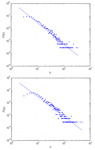
Figure 3 presents the degree distributions of the raw and trend VG networks (2007.9.1-2017.9.1). It can be seen that the degree distributions of both networks obeyed power-law distribution.
As shown in Tables 3 and 4, the degree distributions of the two scale-free networks also obeyed the power law under the five time windows. For both networks, the power-law values were smaller in three windows (2007.9.1-2009.9.1; 2011.9.1-2013.9.1; 2015.9.1-2017.9.1) than in other windows. This is because Wenchuan and Lushan earthquakes and their aftershocks, as near-field earthquakes, release a great deal of energy, inducing great and frequent fluctuations to the WWL in Nanxi Well. In addition, the node degree of the VG with relative large degree, as well as the mean degree of networks <k>, were both on the rise.
The power-law value of the period (2015.9.1-2017.9.1) was small. The WWL variation is not only caused by the Myanmar earthquake, but also the recovery mechanism of the underground system. Overall, the greater the seismic impact on groundwater level, the smaller the power-law values of the VG networks in the time windows. The maximum power-law values appeared in the global VG networks. This means that the seismic impact on the groundwater in global period is not as obvious as that in local periods.
Figure 3. The degree distributions of raw VG network (left) and trend VG network (right)
3.2.3 Assortative mixing
The degree correlations in different time windows can be obtained from Tables 3 and 4. There were three time windows with negative correlations in the raw and trend VG networks: (2007.9.1-2009.9.1; 2011.9.1-2013.9.1; 2015.9.1-2017.9.1). The relevant networks are weak disassortative networks, in which the high degree nodes attach to low degree nodes. During these time windows, Wenchuan earthquake, Lushan earthquake, and Myanmar earthquake took place. The seismic stress of these earthquakes affected the WWL of Nanxi Well. Meanwhile, the number of large degree nodes increased, and the mean and standard deviation of degree were relatively large.
The other two time windows had positive correlations in the raw and trend VG networks: (2009.9.1-2011.9.1; 2013.9.1-2015.9.1). The relevant networks are assertive networks. The seismic waves of the earthquakes that occurred in these periods had relatively limited impact on the WWL of Nanxi Well.
On the global scale (2007.9.1-2017.9.1), the raw VG network was assortative, while the trend VG network was disassortative. This is because the trend time series, which does not contain the interference from barometric pressure, rainfall, and solid tide, amplifies the influence of seismic wave and static stress on WWL fluctuations. The positive and negative degree correlations of different time windows depend on the occurrence of large earthquakes in the response period.
3.2.4 Hierarchy
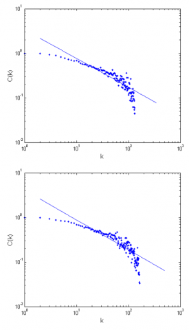
Figure 4 presents the relationship between mean clustering coefficient and node degree in the raw and trend VG networks, separately. The clustering coefficient and degree correlation of each VG network were tested in different time windows. It can be seen that the WWL time series of Nanxi Well were hierarchical networks on both local and global time scales. The hierarchy values are available in Tables 3 and 4. In all the VG networks, low degree cluster centers belonged to small modules with connectivity, while high degree cluster centers linked up different modules into largescale topology modules.
Figure 4. The relationship between mean clustering coefficient and node degree in the raw VG network (left) and the trend VG network (right)
3.2.5 Community
Community is an important measure of the node aggregation in complex networks. Here, the Louvain approach [34] is applied to divide the raw and trend VG networks into multiple communities. Specifically, each network node was treated as an independent community; then, each community moved into another community, only if the move can increase the modularity value; the movement was repeated until no more node moved to other communities. In this way, the raw VG network was divided into 15 communities with the modularity value of 0.7973, and the trend VG network was divided into 17 communities with the modularity value of 0.7627 (Figure 5).
It can be seen from Figure 5 that the communities of the raw VG network were basically the same as those of the trend VG network. There were four relatively large communities related to the recovery period after Wenchuan earthquake, the early stage of Lushan earthquake, the recovery period after Lushan earthquake, and the late stage of Myanmar earthquake, respectively. In the VG network about the WWL time series of Nanxi Well, the community structure depends on the tectonic stress caused by earthquakes. The seismic waves from intermediate- and far-field earthquakes increased the node degree, but did not affect the community division. Similarly, the division of communities was not greatly affected by barometric pressure, rainfall, or soil tide.
Figure 5. The communities of the raw VG network (upper) and the trend VG network (lower)
This paper obtains the trend time series of the WWL by state space model, and applies the VG complex network method to analyze and compare the trend times series and raw time series of the WWL variation induced by 11 earthquakes. The main conclusions are as follows:
(1) In intermediate-field or far-field earthquakes, the WWL recovered in a few days after the seismic waves changed the well permeability. Thus, only a few node degrees increased in the VG networks. By contrast, Wenchuan and Lushan earthquakes pushed up the degrees of many nodes in the raw and trend VG networks. The cluster centers of raw and trend global VG networks are related to the two earthquakes.
(2) All VG networks are scale free. Overall, the greater the seismic impact on groundwater level, the smaller the power-law values of the VG networks in the time windows. The maximum power-law values appeared in the global VG networks. This means that the seismic impact on the groundwater in global period is not as obvious as that in local periods.
(3) The positive and negative degree correlations of different time windows depend on the occurrence of large earthquakes in the response period.
(4) All VG networks are hierarchical. In all the VG networks, low degree cluster centers belonged to small modules with connectivity, while high degree cluster centers linked up different modules into largescale topology modules.
(5) In the VG network about the WWL time series of Nanxi Well, the community structure depends on the tectonic stress caused by earthquakes. The seismic waves from intermediate- and far-field earthquakes increased the node degree, but did not affect the community division. Similarly, the division of communities was not greatly affected by barometric pressure, rainfall, or soil tide.
To sum up, there are close correlations between the large degrees of VG networks, groundwater level variation, and earthquakes. The research findings provide new insights into the WWL response to earthquakes, and the dynamic system of groundwater level fluctuations.
This paper was supported in part by the Earthquake Spark Program Project (Grant No.: XH19070) and National Natural Science Foundation of China (Grant No.: 41877205).
[1] Cooper Jr, H.H., Bredehoeft, J.D., Papadopulos, I.S., Bennett, R.R. (1965). The response of well-aquifer systems to seismic waves. Journal of Geophysical Research, 70(16): 3915-2926. http://doi.org/10.1029/JZ070i016p03915
[2] Rojstaczer, S., (1988). Intermediate period response of water levels in wells to crustal strain: Sensitivity and noise level. Journal of Geophysical Research Solid Earth, 93(B11): 13619-13634. http://doi.org/10.1029/JB093iB11p13619
[3] Eddie, G.Q., Roeloffs, E.A. (1997). Water-level changes in response to the 20 December 1994 Earthquake near Parkfield. Bulletin of the Seismological Society of America, 87(2): 310-317.
[4] Roeloffs, E.A. (1988). Hydrologic precursors to earthquakes: A review. Pure & Applied Geophysics, 126(2-4): 177-209. http://doi.org/10.1007/BF00878996
[5] Gorokhovich, Y. (2005). Abandonment of Minoan palaces on Crete in relation to the earthquake induced changes in groundwater supply. Journal of Archaeological Science, 32(2): 217-222. http://doi.org/10.1016/j.jas.2004.09.002
[6] Wang, C.Y., Manga, M. (2010) Hydrologic responses to earthquakes and a general metric. Front Geofuids, 15: 206-216. https://doi. org/10.1002/9781444394900.ch14
[7] Bosl, W., Nur, A. (2002). Aftershocks and pore fluid diffusion following the 1992 Landers earthquake. Journal of Geophysical Research, 107(B12): 2366. http://doi.org/ 10.1029/2001JB000155
[8] Sibson, R.H., Rowland, J.V. (2003). Stress, fluid pressure and structural permeability in seismogenic crust, North Island, New Zealand. Geophysical Journal International, 154(2): 584-594. http://dx.doi.org/10.1046/j.1365-246X.2003.01965.x
[9] Kinoshita, C., Kano, Y., Ito, H. (2015). Shallow crustal permeability enhancement in central Japan due to the 2011 Tohoku earthquake. Geophysical Research Letters, 42: 773-780. https://doi.org/10.1002/2014GL062792
[10] Igarashi, G., Wakita, H. (1991). Tidal responses and earthquake-related changes in the water level of deep wells. Journal of Geophysical Research Solid Earth, 96(B3): 4269-4278. http://doi.org/0.1029/90JB02637
[11] Matsumoto, N. (1992). Regression and analysis for anomalous changes of ground water level due to earthquakes, Matsumoto, Norio. Regression analysis for anomalous changes of ground water level due to earthquakes. Geophysical Research Letters, 19(12): 1193-1196. http://doi.org/10.1029/92GL01042
[12] Kitagawa, G., Matsumoto, N. (1996). Detection of coseismic changes of underground water level. Journal of the American Statal Association, 91(434): 521-528. http://doi.org/10.1080/01621459.1996.10476917
[13] Matsumoto, N., Kitagawa, G., Roeloffs, E.A. (2003). Hydrological response to earthquakes in the Haibara well, central Japan - I. Groundwater level changes revealed using state space decomposition of atmospheric pressure, rainfall and tidal responses. Geophysical Journal of the Royal Astronomical Society, 155(3): 885-898. http://doi.org/10.1111/j.1365-246X.2003.02103.x
[14] Lacasa, L., Luque, B., Ballesteros, F., Luque, J., Nuno, J.C. (2008). From time series to complex networks: The visibility graph. Proceedings of the National Academy of Sciences of the United States of America, 105(13): 4972-4975. https://doi.org/10.1073/pnas.0709247105
[15] Zhang, B., Wang, J., Fang, W. (2015). Volatility behavior of visibility graph EMD financial time series from Ising interacting system, Physica A, 432(2015): 301-314. http://doi.org/ 10.1016/j.physa.2015.03.057
[16] Zhuang, E. Small, M., Feng, G. (2014). Time series analysis of the developed financial markets’ integration using visibility graphs. Physica A, 410 (2014): 483-495. http://doi.org/ 10.1016/j.physa.2014.05.058
[17] Wang, N., Li, D., Wang, Q. (2012). Visibility graph analysis on quarterly macroeconomic series of China based on complex network theory. Physica A, 391(2012): 6543-6555. http://dx.doi.org/10.1016/j.physa.2012.07.054
[18] Long, Y. (2013). Visibility graph network analysis of gold price time series. Physica A: Statistical Mechanics and Its Applications, 392(16): 3374-3384. http://dx.doi.org/10.1016/j.physa.2013. 03.063
[19] Sun, M., Wang, Y., Gao, C. (2016). Visibility graph network analysis of natural gas price: The case of North American market. Physica A: Statistical Mechanics and its Applications, 462: 1-11. http://dx.doi.org/10.1016/j.physa.2016.06.051
[20] Liu, K., Weng, T., Gu, C., Yang, H. (2020). Visibility graph analysis of Bitcoin price series. Physica A: Statistical Mechanics and its Applications, 538: 122952. http:// dio.org/10.1016/j.physa.2019.122952
[21] Hou, F.Z., Li, F.W., Wang, J. (2016). Visibility graph analysis of very short-term heart rate variability during sleep. Physica A Statistical Mechanics & Its Applications, 458: 140-145. http://doi.org/10.1016/j.physa.2016.03.086
[22] Jiang, S., Bian, C., Ning, X. (2013). Visibility graph analysis on heartbeat dynamics of meditation training. Applied Physics Letters, 102(25): 4972-999. http://doi.org/10.1063/1.4812645
[23] Telesca, L., Lovallo, M., Toth, L. (2014). Visibility graph analysis of 2002-2011 Pannonian seismicity. Physica A, 416: 219-224. http://doi.org/10.1016/j.physa.2014.08.048
[24] Aguilar-San Juan, B., Guzman-Vargas, L. (2013). Earthquake magnitude time series: Scaling behavior of visibility networks. The European Physical Journal B, 86(11): 454. https://doi.org/10.1140/epjb/e2013-40762-2
[25] Xie, W.J., Han, R.Q., Jiang Z.Q (2017). Analytic degree distributions of horizontal visibility graphs mapped from unrelated random series and multifractal binomial measures. EPL (Europhysics Letters), 119(4): 48008. http://dx.doi.org/10.1209/0295-5075/119/48008
[26] Newman, M.E.J., Girvan, M. (2004). Finding and evaluating community structure in networks, Physical Review E: Statistical, Nonlinear, and Soft Matter Physics, 69(2): 026113. http://doi.org/10.1103/physreve.69.026113
[27] Shi, Z. Wang, G. Wang, C.Y. (2014) Comparison of hydrological responses to the Wenchuan and Lushan earthquakes. Earth & Planetary Science Letters, 391: 193-200. http://doi.org/10.1016/j.epsl.2014.01.048
[28] Shi, Z.M., Wang, G.C., Manga, M., Wang, C. Y. (2015). Mechanism of co-seismic water level change following four great earthquakes - insights from co-seismic responses throughout the Chinese mainland. Earth and Planetary Science Letters, 430: 66-74. http://doi.org/10.1016/j.epsl.2015.08.012
[29] Brodsky, E.E., Roeloffs, E., Woodcock, D., Gall, I., Manga, M. (2003). A mechanism for sustained groundwater pressure changes induced by distant earthquakes. Journal of Geophysical Research, 108(B8): 2390. https://doi.org/10.1029/2002JB002321
[30] Roeloffs, E.A. (1998). Persistent water level changes in a well near Parkfield, California, due to local and distant earthquakes. Journal of Geophysical Research Atmospheres, 103(B1): 869-889. http://doi.org/10.1029/97JB02335
[31] Shi, Z., Wang, G. (2014). Hydrological response to multiple large distant earthquakes in the Mile well, China. Journal of Geophysical Research: Earth Surface, 119(11): 2448-2459. http://doi.org/10.1002/2014JF003184
[32] King, C.Y., Azuma, S., Igarashi, G., Ohno, M., Saito, H., Wakita, H. (1999). Earthquake‐related water‐level changes at 16 closely clustered wells in Tono, central Japan. Journal of Geophysical Research: Solid Earth, 104(B6): 13073-13082. http://dx.doi.org/10.1029/1999JB900080
[33] Andrej, M. (2005) Exploratory social network analysis with Pajek. Cambridge University Press.
[34] Blondel, V.D., Guillaume, J.L., Lambiotte, R., Lefebvre, E. (2008). Fast unfolding of communities in large networks. Journal of Statistical Mechanics: Theory and Experiment, 2008(10): 10008. http://doi.org/10.1088/1742-5468/2008/10/p10008