Ganiyu Ayodele Ajibade*![]() | S. A. Olorunsola | Omolayo M. Ikumapayi
| S. A. Olorunsola | Omolayo M. Ikumapayi![]() | Babatope Omolofe | Opeyeolu T. Laseinde
| Babatope Omolofe | Opeyeolu T. Laseinde![]()
© 2024 The authors. This article is published by IIETA and is licensed under the CC BY 4.0 license (http://creativecommons.org/licenses/by/4.0/).
OPEN ACCESS
Control charts have gained increasing attention as a feedback process monitoring technique in recent times. Among them, CUSUM schemes have proven to be effective for monitoring processes with small or moderate sustained mean shifts. However, the detection ability of CUSUM schemes is often slow during the initial process setup due to the constant control limits. To address this limitation, the fast initial response (FIR) or headstart feature has been commonly employed to enhance the scheme's performance at process startup. Additionally, the dynamic nature of real-world challenges calls for a more sensitive CUSUM scheme capable of rapidly identifying small disturbances in a process. In this paper, we propose the utilization of a generalized FIR feature to improve the performance of CUSUM schemes for monitoring process means. By incorporating the generalized FIR feature, we enhance the control limits of the CUSUM scheme, thereby improving its sensitivity to smaller sustained shifts in a process. We assess the efficiency of the proposed system by comparing how well it performs against existing alternatives, using the average run length (ARL), median run length (MDRL), and standard deviation average run length (SDRL) measures. The ARL performance comparison results indicate that the suggested approach shows faster detection of small to moderate sustained alterations in a particular process. Therefore, this method is especially useful for monitoring processes that have observations collected at widely spaced time intervals, such as hourly, daily, or weekly measures, where it is believed that any changes over time will be minor or moderate. To validate the practical viability of our proposed scheme, we showcase its successful implementation in real-world scenarios, utilizing data sets acquired from a beverage bottling company and a petroleum refinery laboratory.
generalized fast initial response for CUSUM charts, small shift detection, process mean monitoring, average run length (ARL), improved CUSUM charts
Process control has garnered significant attention from researchers in various scientific and engineering disciplines in recent years. While numerous tools are available for process control, statistical process control tools like control charts have been widely recognized for their robustness, reliability, and effectiveness. Control charts, including memoryless charts like Shewhart-$\bar{X}$ charts [1], as well as memory-type charts like cumulative sum control charts (CUSUM) initially proposed by Page [2], have been extensively adopted by control practitioners for monitoring industrial processes. Another instance of a memory-based control chart is the exponentially weighted moving average (EWMA) control chart, initially suggested by Roberts [3].
Furthermore, numerous scholars have explored their utility in various domains, in addition to their industrial applications. For instance, Wang and Liang [4] examined its utilization in the field of education. The utilization of control charts in the domains of budgeting, management, and accounting was discussed [5-8]. Furthermore, Hwang et al. [9] explored its utilization in nuclear engineering, while Woodall [10] examined its application in health services. In recent times, the application of SPC to flow meter drift and faulty detection systems has been investigated by Salamah et al. [11] and Benrabah et al. [12] respectively. In addition, the CUSUM scheme as a robustness check for modelling fiscal decentralization and environmental pollution control, and climate monetary policy have been investigated [13, 14]. Other advancements and applications of SPC have been studied in the references [15-22].
Let qt denote the quality variable of interest at time t. Let µ0 and R denote the target and reference values respectively. To monitor the mean of a given process, the upper and lower CUSUMs designed for this purpose are [2]:
$C_t^{+}=\max \left[0, \mathrm{q}_{\mathrm{t}}-\left(\mu_0+R\right)+C_{t-1}^{+}\right]$ (1a)
$C_t^{-}=\max \left[0,\left(\mu_0-R\right)-\mathrm{q}_{\mathrm{t}}+C_{t-1}^{-}\right]$ (1b)
where, $C_0^{+}=C_0^{-}$ are the beginning values that are usually set to zero. Note that max $[a, b]$ returns the maximum of $[a, b]$ for any $a, b \in \Re$ (where $\Re$ is a real number). By designating $H$ as the control threshold. Then, $H$ is defined as
$H=h \sigma$ (2)
where, h and σ are the control limit multiplier and standard deviation of the process respectively. The process will be out-of-control when Ct+ or Ct− exceeds H. Despite CUSUM’s effectiveness at detecting small process changes, its constant control limit has been a major shortcoming, especially at the process startup.
Typically, this reduces the sensitivity of the process at the beginning, which poses a significant economic danger on manufacturing sectors. Any disruptions in the process that go undetected can lead to substantial financial fines. To enhance the sensitivity of CUSUM schemes during the early setup of the process, Lucas and Crosier [23] suggested incorporating the headstart features. This addition aims to further enhance the detecting abilities of CUSUM schemes at the process starting. They introduced nonzero starting values for CUSUM schemes i.e. $C_0^{+}=C_0^{-} \neq 0$. So, under this scheme, the CUSUM chart can be written as
$C_t^{+}=\max \left[C_0^{+}, \mathrm{q}_{\mathrm{t}}-\left(\mu_0+R\right)+C_{t-1}^{+}\right]$ (3a)
$C_t^{-}=\max \left[C_0^{-},\left(\mu_0-R\right)-\mathrm{q}_{\mathrm{t}}+C_{t-1}^{-}\right]$ (3b)
where, the parameters remain the same as in Eq. (1). The only exception is that $C_0^{+}$and $C_0^{-}$ are nonzeros. In some applications, $C_0^{+}$and $C_0^{-}$ are usually set to half of the decision parameter $H$. i.e. $C_0^{+}=C_0^{-}=H / 2$. This is regarded as a $50 \%$ headstart. More details on the choices of $C_0^{+}$and $C_0^{-}$ as the headstart can be found in the research [24].
The remainder of this paper is structured as follows: Section 2 includes CUSUM charts that are based on the modifications of the headstart that varies with time. Section 3 introduces the suggested chart. Section 4 features performance metrics and their evaluation. Section 5 showcases the real-world application of the proposed scheme. Finally, Section 6 concludes.
Research has demonstrated that the persistent FIR characteristic improves the effectiveness of CUSUM schemes. Nevertheless, the immovable nature of CUSUM schemes and their defined control limitations make them less responsive during process starts, which presents a notable danger for processes that are prone to startup problems. Steiner [25] conducted a more in-depth investigation into this subject and expanded on the prior research by Lucas and Crosier [23]. Steiner introduced a time-varying FIR (TFIR) characteristic that tightens the control limit, thereby enhancing the detection capability of the EWMA scheme at the beginning of the process. He demonstrated that the utilization of TFIR-based control limits had a similar effect to the FIR characteristic [23] for the CUSUM scheme.
He suggested the use of the TFIR feature of the form
$\mathrm{FIR}_{\text {adj }}=1-(1-z)^{1+y(t-1)}$. (4)
He suggested that the parameter y, could be set equal to
$y=-\frac{1}{19}\left(1+\frac{2}{\log _{10}(1-z)}\right)$ (5)
So, the control limit for CUSUM under this scheme becomes
$H=h \sigma \mathrm{FIR}_{\text {adj }}$ (6)
Haq et al. [26] improved the FIR characteristic by incorporating a time-varying parameter, thereby further boosting the detection capability of CUSUM and EWMA schemes. He suggests the use of TFIR given as
$\operatorname{MFIR}_{\mathrm{adj}}=\left[1-(1-z)^{1+y(t-1)}\right]^{1+\frac{1}{t}}$ (7)
Thus, the control limit for CUSUM under this scheme becomes
$H=h \sigma \mathrm{MFIR}_{\mathrm{adj}}$ (8)
In either scenario, the process will deviate from in-control if either Ct+ or Ct− exceeds H. These techniques [25-34], have proven effective in enhancing EWMA or CUSUM schemes during the startup phase.
To enable the classical EWMA scheme to revert to its original form after incorporating TFIR characteristics, Ajibade and Ajibade et al. [27, 28] put forward the generalized version of the TFIR (GFIR) for EWMA schemes. In addition, an enhancement parameter for its better performance was given. However, the use of GFIR for the CUSUM scheme has not yet been explored. In this study, we wish to utilize it to improve the CUSUM scheme at the process startup. In the next Section, the design of the GFIR for the CUSUM scheme will be presented.
Let $q_t, t \in \Omega$ be an independent and identical quality variable of interest indexed by the finite index set $\Omega=$ $\left\{t_1, t_2, \ldots, t_s, \ldots, t_n\right\}$ for some $s, n \in \mathbb{N}$, (where $\mathbb{N}$ is a natural number). Note that the index set $\Omega$ contains uniformly spaced time $t$ at which each of the quality variables $q_t$ is realized. Now, assume that $q_t$ is with constant variance $\sigma_q$. Let $\mu_q$ denote the process mean that is obtained by finding the mean of the quality variable $q_t$ Our interest is to promptly detect the time $t$ when the process $q_t$ deviates from $\mu_q$. Let $t_1$ denote the time $t$ at which the process deviates from $\mu_q$. To monitor the process, mean i.e. $\mu_q$, the decision structure is formulated as follows:
$H_0: \mu(t)=\mu_q$ if $t<t_1, t \in \Omega$ (9)
$H_1:$ There exists $t_j^{\prime} \in \Omega$ such that $\mu\left(\mathrm{t}_{\mathrm{j}}^{\prime}\right) \neq \mu_q$, $t>t^{\prime}, \mu\left(t^{\prime}\right)=\mu_1, j=1,2,3, \ldots$ (10)
where, $\mu(.)$ denote the mean of the quality variable at each time t. This structure utilizes a stopping rule which produces a run length $R_L$ or stopping time for the process $q_t, t \in \Omega$ such that the average run length (ARL) is given as
$\operatorname{ARL}(\mu)=\mu_E\left(R_L\right)$
here,$\mu_E$ represents the average or mean of the random number RL relative to the size of the process mean. To enhance the sensitivity of CUSUM charts to these mean shifts, we explore the concept of GFIR, as suggested by Ajibade et al. [28]
$\operatorname{GFIR}_{\mathrm{adj}}=1-(1-z)^{(x+y) t-y}$ (11)
where, $y$ is identical to the one presented in Eq. (5), $z \in$ $[0.1,1]$, and $x$ is the switch parameter. It is thoroughly examined for the EWMA charts [27-30]. For the classical CUSUM chart, we could set $x=t+N(N \geq 400)$. Also, at $x=1 / t$, GFIR${ }_{\text {adj }}$ will perform as FIR${ }_{\text {adj }}$. Note that MFIR${ }_{\text {adj }}$ is $\left(1+\frac{1}{t}\right)$ power exponentiation of FIR${ }_{\text {adj }}$. So, the control limit for the CUSUM charts based on the GFIR${ }_{\text {adj }}$ with the switching parameters described above are the same as the ones given in Eqs. (2) and (4) respectively. To obtain improved FIR-CUSUM charts, we set $x$ equal to
$x=\frac{1+\psi}{t^2}(1-t)$ (12)
So that the control limit for the GFIR-CUSUM scheme becomes
$H=h \sigma\left[1-(1-z)^{(x+y) t-y}\right]$ (13)
where, $x$ is identical to the one presented in Eq. (11). Choosing this value of $x$ considerably tightens the control limit during the initial 14 observations, representing the process startup.
However, decreasing the control limits isn't always beneficial because it inherently leads to quicker detection of process deviations, thereby increasing the chances of encountering a false alarm. Therefore, there exists a compromise between reducing the control limits and keeping them in their original width, known as the traditional CUSUM control limit. However, if there is a need for faster detection of process shifts at commencement, it will be necessary to significantly reduce the control limit at the beginning of the process. The following section will offer the performance measure and analysis.
The assessment of a charting system's performance usually relies on its ARL attributes. ARL denotes the average number of observations needed for a chart to detect a signal. This metric is further divided into two categories: in-control ARL (ARL0) and the out-of-control ARL (ARL1). ARL0 signifies the average number of observations needed to detect an out-of-control signal during normal process operation, whereas ARL1 indicates the average number of observations required to detect an out-of-control signal after the process transitions to an abnormal state. When calculating the ARL, the control limit multiplier (h) is continuously modified in order to attain the required ARL0. Ajibade et al. [28] have recently demonstrated that the steady state-ARL for both the traditional EWMA chart and TFIR-based EWMA schemes are identical. Considering the asymptotic nature of the GFIR, its impact on the control limit of the CUSUM will only affect the observations during the initial phase of the process.
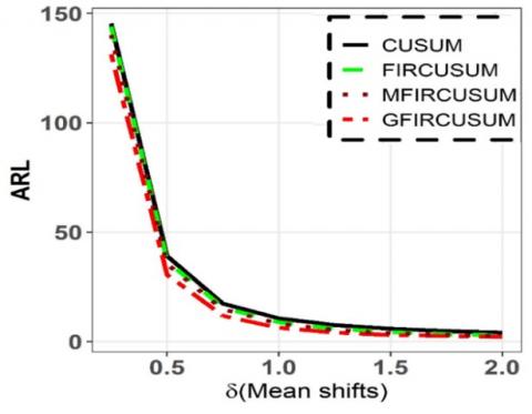
Consequently, the performance measure will only be based on the zero-state ARL. Let's denote the size of sustained shifts in the mean of a process $q_t$ as $\delta$, and let $\sigma_q$ represents the process's standard deviation. We will consider a large number of observations (50000) generated from a standard normal Gaussian process i.e. $q_t \sim N\left(\mu_q+\delta \sigma_q, \sigma_q\right)$, where $\mu_q=0$, $\sigma_q=1$. Here, we use $N$ to represent the standard normal Gaussian process. Our consideration of $\delta$ falls within the interval $0 \leq \delta \leq 2$ (noting that $\delta=0$ indicates the incontrol state, while $\delta>0$ indicates the out-of-control state). By utilizing R-language software, we compute the CUSUM statistics $C_i^{+}$and $C_i^{-}$for these observations using Eq. (1). The control limits specified in Eq. (12) are subsequently imposed on $C_i^{+}$and $C_i^{-}$at every time $t$, with the assumption of an incontrol $\mathrm{ARL}_0=500$. This procedure is iterated 50000 times, tracking the time $t$ (run length) when either $C_i^{+}$or $C_i^{-}$ exceeds the control limit. This iterative process is referred to as a Monte Carlo simulation. Thus, ARL, median run length (MDRL) and standard deviation run length (SDRL) are obtained by taking the average, median and standard deviation of the run length respectively. Table 1 displays the ARL of the proposed scheme alongside its counterparts. The data in Table 1 clearly indicates that the proposed scheme exhibits the lowest $\mathrm{ARL}_1$ values compared to its counterparts. Figure 1 presents the ARL curves of the proposed chart and its counterparts with an in-control $\mathrm{ARL}_0=500$
Table 1. ARL of CUSUM, FIR-CUSUM and GFIR-CUSUM control schemes
|
SCHEME |
CUSUM |
FIR-CUSUM |
MFIR-CUSUM |
GFIR-CUSUM |
|
δ ↓ h→ |
5.0695 |
5.0969 |
5.1124 |
5.2182 |
|
0.000 |
500.766 |
497.209 |
500.129 |
500.460 |
|
0.250 |
145.363 |
143.958 |
140.211 |
131.350 |
|
0.500 |
39.019 |
36.671 |
35.473 |
30.582 |
|
0.750 |
17.336 |
15.504 |
14.713 |
11.789 |
|
1.000 |
10.523 |
8.826 |
8.201 |
6.304 |
|
1.250 |
7.501 |
5.844 |
5.295 |
4.082 |
|
1.500 |
5.820 |
4.320 |
3.849 |
3.036 |
|
1.750 |
4.773 |
3.357 |
2.960 |
2.496 |
|
2.000 |
4.057 |
2.768 |
2.434 |
2.171 |
Figure 1. ARL curves of the proposed chart and its counterparts with an in-control $\mathrm{ARL}_0=500$
Table 2. MDRL of CUSUM, FIR-CUSUM and GFIR-CUSUM control schemes
|
SCHEME |
CUSUM |
FIR-CUSUM |
MFIR-CUSUM |
GFIR-CUSUM |
|
δ ↓ h→ |
5.0764 |
5.0953 |
5.1149 |
5.2243 |
|
0.00 |
348.000 |
346.000 |
343.000 |
324.000 |
|
0.25 |
104.000 |
98.000 |
96.000 |
83.000 |
|
0.50 |
29.000 |
27.000 |
26.000 |
20.000 |
|
0.75 |
14.000 |
13.000 |
12.000 |
7.000 |
|
1.00 |
9.000 |
7.000 |
7.000 |
4.000 |
|
1.25 |
7.000 |
5.000 |
4.000 |
3.000 |
|
1.50 |
5.000 |
4.000 |
3.000 |
2.000 |
|
1.75 |
5.000 |
3.000 |
2.000 |
2.000 |
|
2.00 |
4.000 |
2.000 |
2.000 |
2.000 |
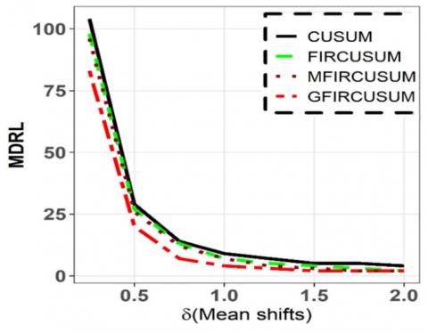
Figure 2. MDRL curves of the proposed chart and its counterparts with an in-control $\mathrm{ARL}_0$= 500
Table 3. SDRL of CUSUM, FIR-CUSUM and GFIR-CUSUM control schemes
|
SCHEME |
CUSUM |
FIR-CUSUM |
MFIR-CUSUM |
GFIR-CUSUM |
|
δ ↓ h→ |
5.0695 |
5.0969 |
5.1124 |
5.2182 |
|
0.00 |
493.945 |
504.521 |
516.235 |
570.418 |
|
0.25 |
137.321 |
142.221 |
142.296 |
149.279 |
|
0.50 |
31.872 |
32.256 |
32.402 |
33.390 |
|
0.75 |
11.214 |
11.681 |
11.901 |
11.816 |
|
1.00 |
5.494 |
5.960 |
6.131 |
5.749 |
|
1.25 |
3.334 |
3.596 |
3.704 |
3.191 |
|
1.50 |
2.267 |
2.464 |
2.485 |
1.883 |
|
1.75 |
1.667 |
1.775 |
1.705 |
1.225 |
|
2.00 |
1.300 |
1.369 |
1.216 |
0.846 |
Figure 3. SDRL curves of the proposed chart and its counterparts with an in-control $\mathrm{ARL}_0$= 500
This implies that the proposed scheme will detect small or moderate shifts in a process mean more quickly. The direct interpretations of the ARLs in the Table 1 are; if the magnitude of the shifts in a process mean is 0.25, it will take about 145 observations for classical CUSUM to detect the shift. Also, for the same magnitude of the mean shift, it will take approximately 143 and 140 observations for FIR-CUSUM and MFIR-CUSUM to detect the shift whereas it will only take approximately 131 observations for GFIR-CUSUM to detect the shift. That means the newly proposed scheme is 9 observations faster than the MFIR-CUSUM scheme, and 14 observations faster than the classical CUSUM scheme. A similar analysis applies to other values of the mean shifts. Additionally, Table 2 presents the MDRL of the proposed chart along with its counterparts. The results also agree with the ARLs. Among the control charts presented, GFIR-CUSUM has the best MDRL values for all the magnitude of the mean shifts. Figure 2 shows the MDRL curves of the proposed chart and its counterparts with an in-control $\mathrm{ARL}_0$= 500.
Finally, Table 3 showcases the SDRL of the proposed scheme and its counterparts. The SDRL value of the proposed scheme is marginally higher than that of its counterparts due to its heightened sensitivity. Figure 3 shows the SDRL curves of the proposed chart and its counterparts with an in-control $\mathrm{ARL}_0$= 500.
In this part, we showcase the real-world application of the newly introduced technique by employing two separate datasets: one containing measurements of bottle filling heights, and the other consisting of Di-glycol amine (DGA) data. The initial dataset is provided as an application-example I, whereas the subsequent dataset is offered as an application-example II.
5.1 Application-example I: vertical dimensions of filled beverage-bottles
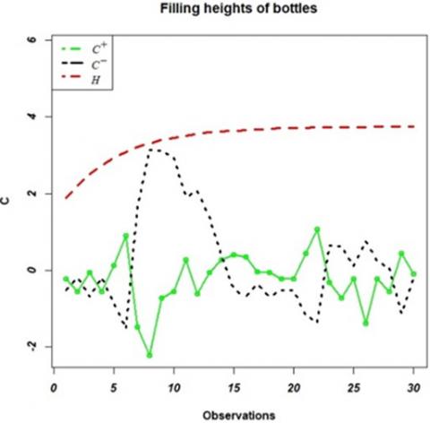
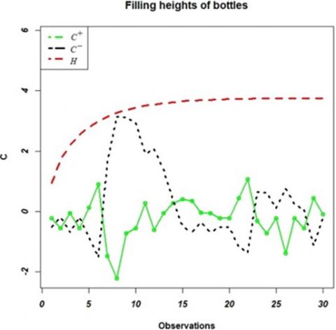
The task of filling empty bottles with soft drinks poses a challenge for bottling companies in the soft drink production process. The fillers simultaneously dispense the beverages into 30 bottles. This dataset is sourced from Ajadi et al. [35]. We observe the dataset utilizing the suggested method and its alternatives by employing Eqs. (1), (2), (6), (8), and (13), along with the decision parameters specified in Table 1. Specifically, the values for k and z are both 0.5, and the control limit multiplier that results in an average run length (ARL0) of 500. The visual depictions are exhibited in Figures 4a-d. It is seen in Figures 4a-c that the process is in-control for CUSUM, FIR-CUSUM and MFIR-CUSUM. However, GFIR-CUSUM is able to locate two out-of-control scenarios at the 8th and 9th observations. These two out-of-control scenarios fall within the startup of the process, hence a corrective action could be made.
(a) CUSUM control chart
(b) FIR-CUSUM control chart
(c) MFIR-CUSUM control chart
(d) GFIR-CUSUM control chart
Figure 4. Application of the proposed chart and its counterparts to bottling data set
5.2 Measurement units and numbers
Di-glycol amine (DGA) is a derivative of amine used in the refinery industry to eliminate Sulfur compounds from petroleum gases via a chemical method called the gas sweetening process. The dataset monitors the precision of the Di-Glycol Amine (DGA) analyzer. Further details about the dataset can be found in Ajadi et al. [36].
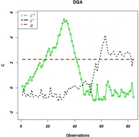
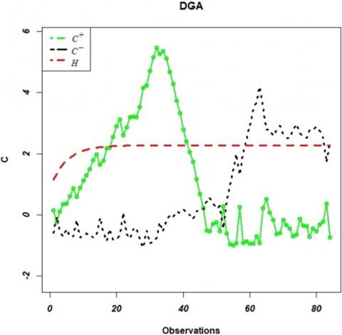
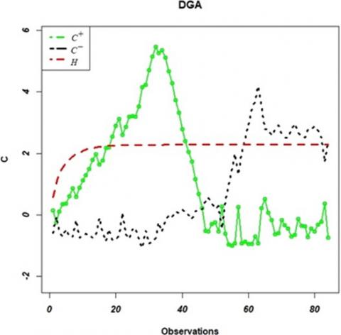
We evaluate the dataset using the suggested scheme and compare it to other schemes using Eqs. (1), (2), (6), (8), and (13), as well as the decision parameters provided in Table 1. Specifically, the values of k and z are both set to 0.5, and the constant h is adjusted to achieve an average run length (ARL0) of 500. The visual depictions are shown in Figures 5a-d. Upon comparing the control charts shown in Figures 5a-d, it is evident that the standard CUSUM, FIR-CUSUM, MFIR-CUSUM, and the suggested GFIR-CUSUM schemes all identify instances of out-of-control scenarios. Specifically, these schemes detect such scenarios between the 19th and 41st observations, as well as between the 59th and 84th observations. This implies that the dataset does not exhibit any initial problems or difficulties. This result is consistent with the conclusion made using EWMA charts [20]. It is worth mentioning the limitations of the proposed monitoring scheme i.e. GFIR-CUSUM. As previously discussed, there is a strong focus on sensitivity during the process startup, while less attention is given to the post-startup phase. Future research should aim to enhance both the process startup and post-startup phases concurrently. One useful suggestion to achieve this could be to implement the dynamic generalized fast initial response method [29].
(a) CUSUM control chart
(b) FIR-CUSUM control chart
(c) MFIR-CUSUM control chart
(d) GFIR-CUSUM control chart
Figure 5. Application of the proposed chart and its counterparts to DGA data set
This work employs generalized quick initial response features to enhance CUSUM schemes. The recently acquired GFIR-CUSUM scheme is extremely responsive to slight or moderate changes in the process mean. We examine the attributes of Average Run Length (ARL), Median Run Length (MDRL), and Standard Deviation of Run Length (SDRL) through the utilization of Monte Carlo simulations. The ARL values suggest that the proposed method can detect shifts in a process mean more rapidly than its predecessors. Moreover, the proposed Scheme exhibits superior Median Run Length (MDRL) values for all the mean shifts. Nevertheless, the SDRLs of this product are slightly elevated compared to its competitors due to its heightened sensitivity.
In order to showcase the implementation of the suggested chart, we utilize actual statistics from bottling corporations and petroleum refinery laboratories to exemplify the tangible utilization of the proposed system. The proposed graphic identified two instances of the bottling process being out of control, while all other charts showed that the process stayed in control. Subsequently, it was discovered that the suggested plan is exceptionally responsive in identifying minor alterations in the process, especially during the first stages. Due to its exceptional sensitivity, the proposed scheme will be highly effective in monitoring processes that experience difficulties during startup, particularly those that require observations at long intervals, such as hours, days, or weeks. Slow detection of changes in the process during these intervals can result in severe consequences.
[1] Shewhart, W.A. (1930). Economic quality control of manufactured product1. Bell System Technical Journal, 9(2): 364-389. https://doi.org/10.1002/j.1538-7305.1930.tb00373.x
[2] Page, E.S. (1954). Continuous inspection schemes. Biometrika, 41(1/2): 100-115. https://doi.org/10.1093/biomet/41.1-2.100
[3] Roberts, S.W. (2000). Control chart tests based on geometric moving averages. Technometrics, 42(1): 97-101. https://doi.org/10.2307/1266443
[4] Wang, Z., Liang, R. (2008). Discuss on applying SPC to quality management in university education. In 2008 The 9th International Conference for Young Computer Scientists, Hunan, China, pp. 2372-2375. https://doi.org/10.1109/ICYCS.2008.301
[5] Albright, T. L., & Roth, H. P. (1993). Controlling quality on a multidimensional level. Journal of Cost Management (Spring), 29-37. https://maaw.info/ArticleSummaries/ArtSumAlbrightRoth93.htm.
[6] Francis, A.E., Gerwels, J.M. (1989). Building a better budget. Quality Progress, 70-75. https://maaw.info/ArticleSummaries/ArtSumFrancisGerwels89.htm.
[7] Holmes, D.S., Hurley, R.E. (2000). How SPC enhances budgeting and standard costing - Another look. Management Accounting Quarterly, 57-62. https://maaw.info/ArticleSummaries/ArtSumHolmesHurley03.htm.
[8] Roehm, H.A., Weinstein, L., Castellano, J.F. (2000). Management control systems: How SPC enhances budgeting and standard costing. Management Accounting Quarterly, 34-40. https://maaw.info/ArticleSummaries/ArtSumRoehmWeinsteinCastellano2000.htm.
[9] Hwang, S.L., Lin, J.T., Liang, G.F., Yau, Y.J., Yenn, T.C., Hsu, C.C. (2008). Application control chart concepts of designing a pre-alarm system in the nuclear power plant control room. Nuclear Engineering and Design, 238(12): 3522-3527. https://doi.org/10.1016/j.nucengdes.2008.07.011
[10] Woodall, W.H. (2006). The use of control charts in healthcare and public-health surveillance. Journal of Quality Technology, 38(2): 89-104. https://doi.org/10.1080/00224065.2006.11918593
[11] Salamah, M.B., Kapoor, A., Savsar, M., Ektesabi, M., Abdekhodaee, A., Shayan, E. (2011). The detection of flow meter drift by using statistical process control. International Journal of Sustainable Development and Planning, 6(1): 91-103. https://doi.org/10.2495/SDP-V6-N1-91-103
[12] Benrabah, M.E., Kadri, O., Mouss, K.N., Lakhdari, A. (2022). Faulty detection system based on SPC and machine learning techniques. Revue d'Intelligence Artificielle, 36(6): 969-977. https://doi.org/10.18280/ria.360619
[13] Omodero, C.O. (2021). Fiscal decentralization and environmental pollution control. International Journal of Sustainable Development and Planning, 16(7): 1379-1384. https://doi.org/10.18280/ijsdp.160718
[14] Omodero, C.O., Alege, P.O. (2023). Climate monetary policy design and modelling. International Journal of Design & Nature and Ecodynamics, 18(1): 175-181. https://doi.org/10.18280/ijdne.180121
[15] Abikenova, S., Aitimova, S., Daumova, G., Koval, A., Sarybayeva, I. (2023). Statistical monitoring of OSH: Analysis of deviations and recommendations for optimization. International Journal of Safety and Security Engineering, 13(6): 1049-1059. https://doi.org/10.18280/ijsse.130607
[16] Ipek, H., Ankara, H., Ozdag, H. (1999). The application of statistical process control. Minerals Engineering, 12(7): 827-835. https://doi.org/10.1016/S0892-6875(99)00067-9
[17] Madanhire, I., Mbohwa, C. (2016). Application of statistical process control (SPC) in manufacturing industry in a developing country. Procedia CIRP, 40: 580-583. https://doi.org/10.1016/j.procir.2016.01.137
[18] Vander Wiel, S.A., Tucker, W.T., Faltin, F.W., Doganaksoy, N. (1992). Algorithmic statistical process control: Concepts and an application. Technometrics, 34(3): 286-297. https://doi.org/10.1080/00401706.1992.10485278
[19] Cook, G.E., Maxwell, J.E., Barnett, R.J., Strauss, A.M. (1997). Statistical process control application to weld process. IEEE Transactions on Industry Applications, 33(2): 454-463. https://doi.org/10.1109/28.568010
[20] Doumani, I., Pujo, P., M'Sirdi, N. (2016). Detection of process microdefects, within the warning limits of a control chart: Application to the wafer manufacturing in the semiconductor industry. Journal Europeen des Systemes Automatises, 49(2): 161-180. https://doi.org/10.3166/JESA.49.161-180
[21] Boregowda, S., Handy, R., Bae, E., Whitt, M. (2023). Entropic characterization of multiple physiological responses with statistical process control charts. International Journal of Design & Nature and Ecodynamics, 18(2): 335-340. https://doi.org/10.18280/ijdne.180210
[22] Maryani, E., Purba, H.H., Sunadi. (2021). Analysis of aluminium alloy wheels product quality improvement through DMAIC method in casting process: A case study of the wheel manufacturing industry in Indonesia. Journal Européen des Systèmes Automatisés, 54(1): 55-62. https://doi.org/10.18280/jesa.540107
[23] Lucas, J.M., Crosier, R.B. (1982). Fast initial response for CUSUM quality-control schemes: Give your CUSUM a head start. Technometrics, 3(24): 199-205. https://doi.org/10.2307/1271440
[24] Montgomery, D.C. (2019). Introduction to Statistical Quality Control. John Wiley & Sons.
[25] Steiner, S.H. (1999). EWMA control charts with time-varying control limits and fast initial response. Journal of Quality Technology, 31(1): 75-86. https://doi.org/10.1080/00224065.1999.11979899
[26] Haq, A., Jennifer, B., Moltchanova, E. (2013) Improved fast initial response features for exponentially weighted moving average and cumulative sum control charts. Quality and Reliability Engineering International, 5(30): 697-710. https://doi.org/10.1002/qre.1521
[27] Ajibade, G.A. (2016). A Multiobjective optimization design for statistical process control. King Fahd University of Petroleum and Minerals, Dhahran, Saudi Arabia.
[28] Ajibade, G.A., Riaz, M., Alshahrani, M., Kuboye, J.O., Alih, E., Ajadi, J.O. (2022). Generalization of time-varying fast initial response for exponentially weighted moving average control charts. Quality and Reliability Engineering International, 38(8): 4157-4168. https://doi.org/10.1002/qre.3194
[29] Ajibade, G.A., Enoch, O.O. (2023). Dynamic generalized fast initial response for EWMA control schemes for monitoring processes with startup and post-startup problems. Quality and Reliability Engineering International, 39(3): 922-930. https://doi.org/10.1002/qre.3269
[30] Ajibade, G.A., Ajadi, J.O., Kuboye, J.O., Alih, E. (2023). Generalized new exponentially weighted moving average control charts (NEWMA) for monitoring process dispersion. International Journal of Quality & Reliability Management. https://doi.org/10.1108/IJQRM-08-2022-0257
[31] Lucas, J.M., Saccucci, M.S. (1990). Exponentially weighted moving average control schemes, properties and enhancements. Technometrics, 32(1): 1-29. https://doi.org/10.2307/1269841
[32] Knoth, S. (2005). Fast initial response features for EWMA control charts. Statistical Papers, 46: 47-64. https://doi.org/10.1007/BF02762034
[33] Pokojovy M., Jobe, G.M. (2021). Univariate fast initial response statistical process control with taut strings. Journal of Applied Statistics, 49(9): 2326-2348. https://doi.org/10.1080/02664763.2021.1900798
[34] Rhoads, T.R., Montgomery, D.C., Mastrangelo, C.M. (2007). A fast initial response scheme for the exponentially weighted moving average control chart. Quality Engineering, 9(2): 317-327. https://doi.org/10.1080/08982119608919048
[35] Ajadi, J.O., Riaz, M., Al-Ghamdi, K. (2016). On increasing the sensitivity of mixed EWMA-CUSUM control charts for location parameter. Journal of Applied Statistics, 43(7): 1262-1278. https://doi.org/10.1080/02664763.2015.1094453
[36] Ajadi, N.A., Asiribo, O., Dawodu, G. (2020) Progressive mean exponentially weighted moving average control chart for monitoring the process location. International Journal of Quality & Reliability Management, 38(8): 1680-1694. https://doi.org/10.1108/IJQRM-05-2020-0138