Mounia Hendel*![]() | Khadra Kessairi
| Khadra Kessairi![]() | Mostefa Brahami
| Mostefa Brahami![]() | Abderrezak Mansouri
| Abderrezak Mansouri![]()
© 2024 The authors. This article is published by IIETA and is licensed under the CC BY 4.0 license (http://creativecommons.org/licenses/by/4.0/).
OPEN ACCESS
The breakdown voltage characterizes the required voltage at which an electrical insulator will become a conductor of electricity. Measurements of short air gap discharge voltages are essential to guarantee safety, compliance and reliability in electrical energy transmission and transformation networks. After the implementation of three distinct neural models for three short air gap configurations prediction: Electrode-Sphere-Sphere-Earth (ESSE), Electrode-Sphere-plane (ESP), and Electrode-Symmetry-Sphere (ESS); the present research introduces an innovative compact and intelligent architecture to predict the breakdown voltages of any short air gap configuration (without having to resort to reconfiguring the system each time), based on a universal automatic multi-layer neural network (MLP) repressor. The unified architecture receives as input the radius, distance and indicator of the configuration and returns as output the predicted breakdown voltage. Our system has been validated on three configurations (with several internal diameter electrodes) and a fairly rich database (taken from the literature) with a Mean Square Error (MSE) of around 11.84%, which certify the yield of the methodology undertaken.
automatic regression, MLP neural network, short air gap, gradient backpropagation, breakdown voltage
Electrical insulation is an elementary characteristic when designing and implementing electrical systems, whose aim is to guarantee the separation of conductor or electrical constituents. This will prevent, any unwanted or unexpected contact that can lead to electric shocks, short circuits, or other unappreciated phenomena resulting from electricity circulation. The breakdown voltage represents the maximum voltage limit that an insulating material can withstand before suddenly losing its insulating properties and becoming conductive. This phenomenon's consequences are multiple: irreversible damage to the insulation compromising its insulation capacity, short circuits between conductors leading to electrical equipment malfunctions, etc. This damage can lead to a power supply interruption, which can have significant repercussions in critical areas [1-3].
Like any gaseous medium, atmospheric air is considered an insulator. In an aerial network, the air is subjected to sufficient electrical voltage. In the presence of impurities and severe atmospheric conditions, a current of electrically charged particles becomes possible through the medium partial ionization [4-6]. Consequently, the air becomes conductive, which leads to breakdown. Alternatives and models for estimating electrical breakdown voltages are in high demand for areas involving electrical insulation, more particularly, in energy transportation and distribution networks; The models allow, in fact, to predict with certainty the electrical equipment sizing, to develop efficient technologies for preventing atmospheric discharges, and to accurately deduce safety distances.
The study of breakdown in air gaps has been the subject of several research in recent years. However, the airflow mechanism still needs to be fully understood. Methods for measuring breakdown voltage are subdivided into two approach categories: conventional methods (experimentally and theoretical) [7-10] and methods based on Artificial Intelligence (AI). Traditional methods of measuring breakdown voltage have certain disadvantages. On the one hand, these methods involve sophisticated equipment and require complex installations (such as special measuring chambers), thus making their implementation very expensive and limiting their accessibility and use. On the other hand, the results obtained are hazardous and of limited use due to the atmospheric conditions influence and the discharge energy influence on the samples studied. These drawbacks push the scientific community to intensify their research in order to propose more ingenious, efficient and economical breakdown measurement approaches. AI methods, inspired by living things' reasoning mechanisms, are seen as a critical solution due to the multitude of significant advantages they present. Indeed, AI promises to save time through the automation of the estimation process. AI ensures accurate, reliable results and reduces computing costs by eliminating expensive devices. Finally, AI has the particularity of learning from experience and adapting to situations never seen before, which makes it very suitable for the problem of approximating the electrical insulators' breakdown voltages, particularly air. With this in mind, several ingenious research in the field of breakdown voltage estimation based on intelligent regression approaches have been proposed, including those based on neural networks [11-15], those based on Support Vector Regression (SVR) [16-20], those based on Support Vector Machine (SVM) [11, 21, 22], those based on fuzzy logic [23, 24] and those based on extremely randomized trees algorithm [11]. In what follows, we will detail some studies that are pretty similar to ours:
A thorough analysis of the intelligent systems proposed previously allowed us to raise the following limits: (1) Unlike MLP, RBF is generally favorable for studies whose training sample numbers are quite limited; however, it is necessary to improve them by optimization techniques and vector quantification otherwise. (2) SVR remains favorable in both cases. Nevertheless, their rather complex mathematical foundation and the need to adjust their hyper parameters make their implementation very difficult and expensive in terms of implementation time. (3) The SVM use based on the translation of a regression problem to a classification problem is a bad idea because the obtained results will be non-precise and bounded in an interval. (4) Fuzzy logic is a compelling alternative. However, it remains based on the living beings' logical reasoning, which can make it ineffective in the face of unforeseen situations. In this study, we opted for using MLP because, on the one hand, we have a reasonably rich database which will allow us to train them well; and on the other hand, MLP-type neural networks offer a multitude of advantages, including: adaptability, non-linear data management, ability to extract characteristics from noisy data, robustness to noisy data, effectiveness for regression problems and performance improvement with the data quantity augmentation, etc.
Furthermore, the state of the art allowed us to conclude that despite the existence of a multitude of approaches to estimate the breakdown voltage of different air gap configurations and despite the existence of models which will enable switching between one configuration to another by taking only one configuration at a time. It isn't easy to find models that can guarantee the ability to easily adapt to additions of configurations (the possibility of extending the model) in a relatively simple way (natural, flexible and intuitive) without having to resort to neglecting configurations previously implemented in the same model. The only researches found are that of the studies [21, 22], which proposes a system that manages several configurations at the same time. All the same, this system remains primarily based on breakdown voltage estimation techniques based on mathematical and experimental calculation models (the disadvantages of which are cited above in the introduction); the SVM are only used to refine the tensions already obtained with precision. Furthermore, despite the good results obtained, the implemented systems remain quite complicated and require a fairly long execution time.
In this sense, the present study first presents a unique configuration based on MLP (in adequacy with existing models), with the aim of separately approaching the breakdown voltages of three distinct air gap configurations: Electrode-Sphere-Sphere-Earth (ESSE), Electrode-Sphere-plane (ESP), Electrode-Symetry-Sphere (ESS). Subsequently, the novelty of this research lies in the proposition of a new 100% intelligent unifier architecture is proposed to support all the air gap configurations studied. Thus, the proposed unified model has as first objective to propose a simple and flexible architecture 100% intelligent, which allows a fluid extension of the model to manage other configuration types. The model has as second objective to propose an efficient estimator with the speed and the precision of calculation, which will allow to consider an integration in real time/processes.
This paper is organized as follows: Section 2 will be devoted to the used database presentation. Section 3 will be dedicated to a brief description of the MLP mathematical foundation, followed by a well-established description of the proposed unified model. Section 4 will be reserved for the listing and discussion of the obtained results. Section 5 of this paper will serve as a conclusion.
Table 1. Training and estimation examples distribution according to each configuration
|
Configuration Type |
Examples Numbers According to the Sphere Radius |
|||||
|
a=250 mm |
a=125 mm |
a=62.5 mm |
a=31.25 mm |
Total examples number |
||
|
ESSE |
29 |
16 |
12 |
8 |
65 |
|
|
Learning: 50.77% |
Test: 49.23% |
|||||
|
ESP |
30 |
22 |
15 |
- |
67 |
|
|
Learning: 50.76% |
Test: 49.24% |
|||||
|
ESS |
- |
29 |
18 |
11 |
58 |
|
|
Learning: 50.72% |
Test: 48.28% |
|||||
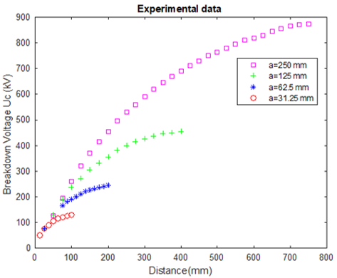
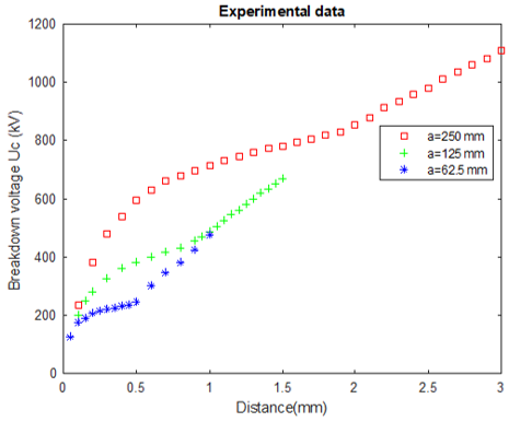
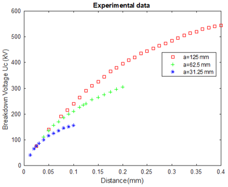
We have a database made up of 190 examples taken from the research work of Donohoe et al. [25]. Three electrode configurations are considered in this study for the test and training samples construction:
The distribution of test and training sample distributions is presented in Table 1 and Figures 1-4 in accordance with the configurations considered. For each configuration and each diameter, the data sets were split into two: a training set and an estimation set.
Before splitting the global base, a centred/reduced normalization process (Eq. 1) was applied in order to keep the same distribution for all samples. The normalization is done separately by taking into consideration each configuration sample for the unique estimators, and the normalization is done on a global basis for the proposed hybrid estimator implementation.
$\widetilde{x_{i j}}=\frac{\left(x_{i j}-\overline{x_j}\right)}{\sigma_{x j}}$ (1)
where, $\overline{x_j}$ is the mean and $\sigma_{x j}$ is the standard deviation.
Figure 1. Experimental examples distribution (ESSE configuration)
We note that other normalization techniques have been tested, namely "Min-Max normalization" (Eq. 2) and "Log transformation" (Eq. 3). The three normalization approaches were applied to the data set considered in this study, to obtain new normalized sets; the approximators performances were then evaluated based on each new set. For all configurations, the test results obtained with "centred/reduced normalization" reflected a significant reduction in the estimation error compared to other techniques.
$x_{i j}^{\prime}=\frac{x_{i j}-\min \left(x_j\right)}{\max \left(x_j\right)-\min \left(x_j\right)}$ (2)
$x_{i j}^{\prime}=\log \left(x_{i j}\right)$ (3)
Figure 2. Experimental examples distribution (ESP configuration)
Figure 3. Experimental examples distribution (ESS configuration)
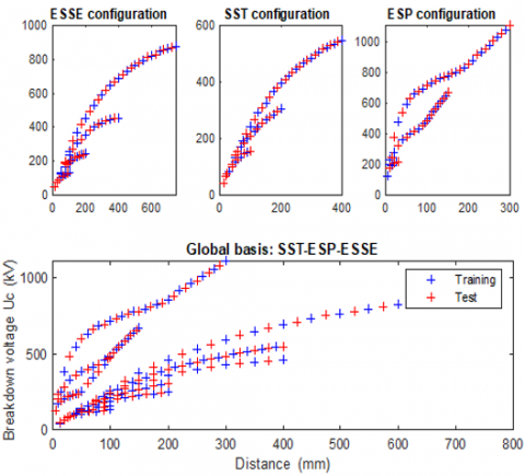
Figure 4. Training and estimation examples distribution (unique configuration)
MLP is a supervised learning model with high computational capacity. Its structure consists of an “input layer”, an “output layer” (interpreted as the response of the network) and one or more intermediate layers called “hidden layers”. A neuron in the bottom layer can only be connected to neurons in subsequent layers. In this study, the MLP is considered for the breakdown voltages calculation in short air gap configurations; it is, in fact, a regression problem.
The regression model hyperparameters selection is a crucial and essential step for an intelligent mathematical model design, capable of behaving effectively in the face of test examples never before seen. For an MLP type approximator, the optimized parameters are those relating to: hidden layer number, the hidden layer neuron number, the activation functions, the metric chosen for the learning error evaluation and the learning algorithm.
3.1 Gradient back propagation algorithm
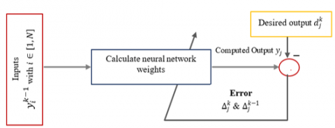
In the multilayer network structure, the gradient back propagation method is most frequently used to minimize the Mean Square Error (MSE) between the network output and the desired output. This algorithm back-propagates the error gradient from the output to the input. This operation is repeated until the difference between the network output and the desired output becomes acceptable (Figure 5).
Figure 5. Synaptic weights modification in supervised learning
Learning by backpropagation is carried out in successive steps, which are described above [26, 27]:
1) The synaptic coefficients are initialized with small random values (NB: large values tend to cause the activation functions to become saturated).
2) Presentation of the characteristic vectors as input to the classifiers.
3) Iteratively calculate the neuron states in the following layers using Eq. (2).
$y_j^k=f\left(\sum_{i=1}^N w_{j i}^k \cdot y_i^{k-1}\right)$ (4)
with:
$f$: activation function.
$N$: neurons number in layer k-1.
$k$: current layer number.
$y_j^k$: output of neuron j from layer k.
$w_{j i}^k$: connection between neuron i of layer k-1 and neuron j of layer k.
$y_i^{k-1}$: output of neuron $i$ from layer k-1.
4) Calculation of the error gradient made on neuron i in the output layer:
$\Delta_j^k=2 f^{\prime}\left(\sum w_{j k}^k \cdot y_j^{k-1}\right) \cdot\left(d_j^k-y_i^k\right)$ (5)
with:
$f^{\prime}$: the derivative of the function f.
$d_j^k$: the desired output for neuron i in layer k.
5) Back-propagated error gradients calculation from layer k to layer 1:
$\Delta_j^{k-1}=2 f^{\prime}\left(\sum_{i=1}^N w_{j k}^k \cdot y_j^{k-1}\right) \cdot \sum_{i=1}^N \Delta_j^k w_{j i}^k$ (6)
6) Synaptic coefficients update:
$w_{j i}^k(t+1)=w_{j i}^k(t)+\Delta \cdot \delta_j^k \cdot y_j^k$ (7)
with:
$\Delta$: is the gradient step.
Repeat all steps, except the first, each time for a new characteristic vector, until the stop test is activated.
3.2 MLP for a separate configuration breakdown voltage estimating
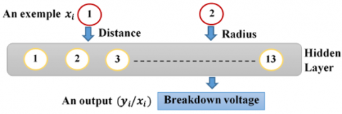
This sub-section will be devoted to presenting the methodology adopted to implement our unique intelligent estimators, each of which is responsible for interpolating the breakdown voltages of a single electrode geometry configuration. Each selected architecture is a three-layer configuration (Figure 6):
- An input layer: made up of two neurons, the first receiving the distance, and the second receiving the radius.
- A single hidden layer: the number of which is fixed empirically by testing several values and keeping the one that gave the best result (Table 2).
- An output layer is made up of a single neuron that returns the estimated breakdown voltage.
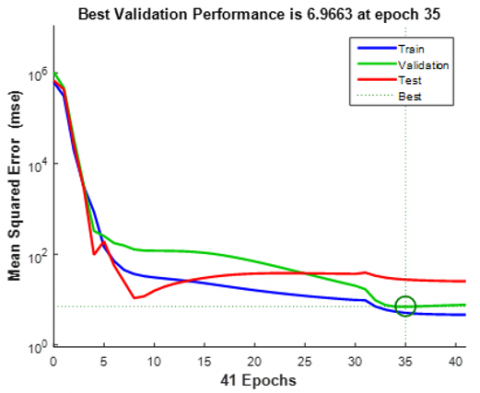
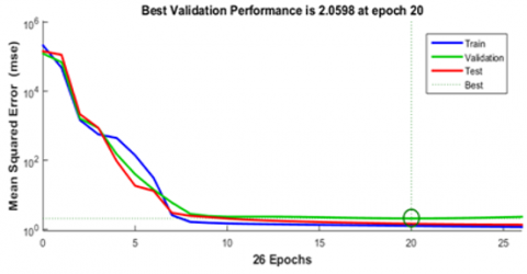
The MSE evaluation is shown in Figures 7-9. From the three figures, we can see a perfect convergence with quadratic errors, which are of the order of ESSE: 6.295, ESP: 6.966 and ESS: 2.0598. These findings prove the effectiveness of the unique configurations proposed.
3.3 MLP unified model
The goal of this section is to propose a compact architecture that makes it possible to address the problem in its entirety by supporting all three configurations (ESSE, ESP, and ESS). The training and testing data are the concatenation of the sets used to train and test the networks of the three configurations (ESSE, ESP and ESS) individually. The development of this unique network (see Figure 10) requires:
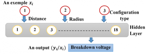
- There are three input neurons: one that receives the distance from which we want to estimate the breakdown voltage, one that receives the radius, and one that receives the configuration type (1 for SST, 2 for ESP, and 3 for ESS).
- One hidden layer whose neuron number was fixed empirically by testing several values and keeping the one that gave the best result (Table 3).
- A single output neuron that gives the estimated breakdown voltage.
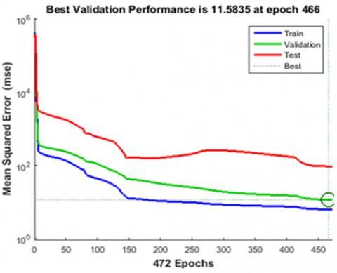
The squared error during the iterations is schematized in Figure 11. We see a very satisfactory convergence (with an MSE of around 11.5835), which once again proves the effectiveness of the proposed configuration.
Figure 6. Graphical representation of the single model's configuration
Figure 7. MSE error evolution during the iteration (ESSE configuration)
Figure 8. MSE error evolution during the iteration (ESP configuration)
Figure 9. MSE error evolution during the iteration (ESS configuration)
Figure 10. Graphical representation of the unique model configuration
Table 2. MSE evolution according to the hidden layer neurons number
|
Neurons Number |
5 |
7 |
9 |
11 |
13 |
15 |
17 |
19 |
21 |
23 |
25 |
27 |
29 |
|
ESSE |
33.20 |
37.19 |
19,88 |
11.65 |
6.29 |
8.64 |
9.76 |
22.18 |
25.23 |
16.15 |
32.23 |
33.31 |
34.86 |
|
ESP |
29.85 |
35.10 |
18.85 |
12.72 |
6.96 |
9.66 |
10.62 |
26.84 |
23.24 |
17.55 |
33.41 |
31.47 |
35.85 |
|
ESS |
5.92 |
3.78 |
2.96 |
4.42 |
2.05 |
3.57 |
4.65 |
3.01 |
4.30 |
3.59 |
5.61 |
5.10 |
6.66 |
Table 3. MSE evolution according to the hidden layer neurons number
|
Neurons Number |
8 |
10 |
12 |
14 |
16 |
18 |
20 |
22 |
24 |
26 |
|
MSE |
62.19 |
46.25 |
46.39 |
96.81 |
21.65 |
11.58 |
16.79 |
28.78 |
35.48 |
48.98 |
Figure 11. MSE error evolution during the iteration (unique configuration)
This section presents the obtained results after learning our different unique models and the proposed global model.
4.1 Electrode-Sphere-Sphere-Earth (ESSE)
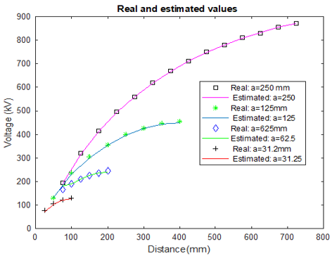
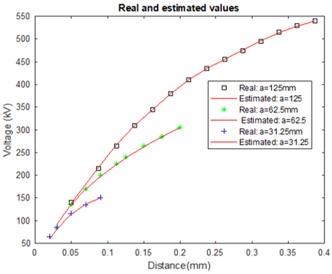
After the learning phase comes the test phase, from which the estimator performance is tested, Figure 12 illustrates the obtained results in the test phase. The outputs given by the network coincide in the majority of cases with the desired outputs with an MSE of 6.71%.
In order to properly view and analyse the obtained results, we list in Table 4 the obtained estimates and the estimation error for each distance. We see that the testing errors for all the sphere radius are insignificant and almost zero. This underlines the undertaken approach effectiveness and also proves the efficient execution of the model training phase.
4.2 Electrode-Sphere-plane (ESP)
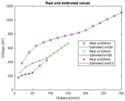
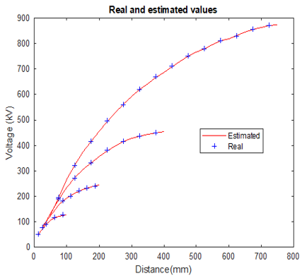
Once the network was trained, we presented it with all the experimental test data; the network responses are listed in Table 5 and Figure 13.
We notice from the obtained test results that the calculated output and the expected output are practically identical with an equal MSE to 7.15%. This confirms that the proposed network is well-trained and is able to behave effectively when faced with new examples.
Figure 12. Obtained test results by the proposed architecture (ESSE configuration)
Table 4. Error in test (ESSE configuration)
|
Sphere Radius 250 mm |
||||||||||||||
|
Estimated output |
193 |
317 |
416 |
490 |
558 |
622 |
675 |
711 |
747 |
780 |
805 |
832 |
856 |
871 |
|
Desired output |
195 |
320 |
415 |
495 |
560 |
620 |
670 |
710 |
750 |
780 |
810 |
830 |
855 |
870 |
|
Error |
2 |
3 |
-1 |
5 |
2 |
-2 |
-5 |
-1 |
3 |
0 |
5 |
-2 |
-1 |
-1 |
|
Sphere Radius 125 mm |
||||||||||||||
|
Estimated output |
133 |
230 |
301 |
355 |
396 |
425 |
444 |
|
|
|
|
|
|
|
|
Desired output |
130 |
235 |
305 |
355 |
400 |
425 |
445 |
|
|
|
|
|
|
|
|
Error |
-3 |
5 |
4 |
0 |
4 |
0 |
1 |
|
|
|
|
|
|
|
|
Sphere Radius 62.5 mm |
||||||||||||||
|
Estimated output |
166 |
191 |
210 |
225 |
236 |
240 |
|
|
|
|
|
|
|
|
|
Desired output |
165 |
190 |
210 |
225 |
235 |
245 |
|
|
|
|
|
|
|
|
|
Error |
-1 |
-1 |
0 |
0 |
-1 |
5 |
|
|
|
|
|
|
|
|
|
Sphere Radius 31.25 mm |
||||||||||||||
|
Estimated output |
77 |
105 |
122 |
131 |
|
|
|
|
|
|
|
|
|
|
|
Desired output |
75 |
105 |
120 |
130 |
|
|
|
|
|
|
|
|
|
|
|
Error |
-2 |
0 |
-2 |
-1 |
|
|
|
|
|
|
|
|
|
|
Table 5. Error in test (ESP configuration)
|
Sphere Radius 250 mm |
|||||||||||||||
|
Estimated output |
379 |
544 |
629 |
679 |
715 |
744 |
771 |
794 |
817 |
853 |
911 |
965 |
1014 |
1057 |
1109 |
|
Desired output |
380 |
540 |
630 |
680 |
715 |
745 |
775 |
795 |
820 |
855 |
915 |
960 |
1010 |
1060 |
1110 |
|
Error |
1 |
-4 |
1 |
1 |
0 |
1 |
4 |
1 |
3 |
2 |
4 |
-5 |
-4 |
3 |
1 |
|
Sphere Radius 125 mm |
|||||||||||||||
|
Estimated output |
247 |
330 |
380 |
413 |
457 |
489 |
526 |
563 |
600 |
635 |
672 |
|
|
|
|
|
Desired output |
250 |
325 |
380 |
415 |
455 |
485 |
525 |
560 |
600 |
635 |
670 |
|
|
|
|
|
Error |
3 |
-5 |
0 |
2 |
-2 |
-4 |
-1 |
-3 |
0 |
0 |
-2 |
|
|
|
|
|
Sphere Radius 62.5 mm |
|||||||||||||||
|
Estimated output |
171 |
205 |
218 |
229 |
248 |
343 |
427 |
|
|
|
|
|
|
|
|
|
Desired output |
175 |
205 |
220 |
230 |
245 |
345 |
425 |
|
|
|
|
|
|
|
|
|
Error |
4 |
0 |
2 |
1 |
-3 |
2 |
-2 |
|
|
|
|
|
|
|
|
Figure 13. Obtained test results by the proposed architecture (ESP configuration)
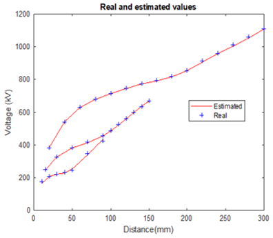
Figure 14. Obtained test results by the proposed architecture (ESS configuration)
Table 6. Error in test (ESS configuration)
|
Sphere Radius 125 mm |
||||||||||||||
|
Estimated output |
137 |
218 |
265 |
307 |
345 |
379 |
409 |
435 |
459 |
479 |
497 |
513 |
527 |
540 |
|
Desired output |
140 |
215 |
265 |
310 |
345 |
380 |
410 |
435 |
455 |
475 |
495 |
515 |
530 |
540 |
|
Error |
3 |
-3 |
0 |
3 |
0 |
1 |
1 |
0 |
-4 |
-4 |
-2 |
2 |
3 |
0 |
|
Sphere Radius 62.5 mm |
||||||||||||||
|
Estimated output |
88 |
133 |
171 |
201 |
227 |
241 |
265 |
285 |
305 |
|
|
|
|
|
|
Desired output |
85 |
135 |
170 |
200 |
225 |
240 |
265 |
285 |
305 |
|
|
|
|
|
|
Error |
-3 |
2 |
-1 |
-1 |
-2 |
-1 |
0 |
0 |
0 |
|
|
|
|
|
|
Sphere Radius 31.25 mm |
||||||||||||||
|
Estimated output |
63 |
85 |
115 |
134 |
152 |
|
|
|
|
|
|
|
|
|
|
Desired output |
65 |
85 |
115 |
135 |
150 |
|
|
|
|
|
|
|
|
|
|
Error |
2 |
0 |
0 |
1 |
-2 |
|
|
|
|
|
|
|
|
|
4.3 Electrode-Symmetry-Sphere (ESS)
At the end of the learning phase of this new geometry configuration, the test examples were presented as input to the regression model; the breakdown voltages estimated by the network in the test phase are listed in Table 6 and Figure 14 (separately for each sphere radius).
The test results show that the calculated output and the expected output are practically identical with an MSE equal to 3.82%, this confirms that the proposed network is well-trained and can behave effectively when faced with new examples; and once again prove the effectiveness of: the two input choices, the adopted procedure to choose the hidden layer neuron numbers and the learning procedure.
4.4 Unified configuration
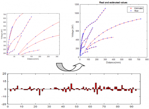
Once the network was trained, we tested it by first presenting the test data for each configuration individually (Figures 15-17) and then all the experimental data (Figure 18), the error representation is also shown in Figure 18. The obtained results reflect in the majority of cases, an estimated tension that coincide with the real values with an MSE of around of 11.84%.
In conclusion, we note that the proposed hybrid model, which is based mainly on a universal MLP-type estimator trained with the gradient back-propagation algorithm, effectively addresses the problem of estimating the breakdown voltage from the distance between electrodes; since, in all cases, the error between the actual breakdown voltage and the estimated voltage does not exceed 10 KV. Theoretically these results are very encouraging; in the worst case an error of 10 KV for example, for a breakdown voltage of 380 KV is insignificant since the error only represents 2.65% of the overall percentage.
4.5 Comparative analysis
A comparative study is necessary to position this study in relation to the studies previously proposed in the literature. However, it is not apparent to favour one result or another; several parameters must be taken into consideration. So, for comparison, Table 7 below illustrates the results of some studies similar to ours from the point of view of the following: considered configuration type, concerned configuration number at the same time, air gap type, and MSE error.
Figure 15. Obtained test results by the proposed unified architecture (ESSE configuration)
Figure 16. Obtained test results by the proposed unified architecture (ESP configuration)
Figure 17. Obtained test results by the proposed unified architecture (ESS configuration)
Figure 18. Global obtained test results by the proposed unified architecture (for all configurations)
Table 7. Comparative analysis
|
Study |
Configuration Type |
Configuration Number |
Air Gap Type |
Samples Number |
MSE Error |
|
CS-ω-SVR [16, 17] |
rod-rod |
One configuration at a time |
Long gap |
14 |
8.8 |
|
MLP [12] |
point-barrier |
One configuration at a time |
Not mentioned |
Not mentioned |
9.91 |
|
RBF-ROM [15] |
barrier-point-plane |
One configuration at a time |
Long gap |
$\simeq$ 50 |
5.8 |
|
EF-SVM [21] |
sphere-sphere, rod-plane, sphere-plane and sphere-plane-sphere |
four configurations at a time |
Short gap |
25 |
4.12 |
|
EF-OD-SVM [22] |
sphere-sphere, rod-plane and rod-gaps between rods |
three configurations at a time |
Short gap |
99 |
6.86 |
|
IRM-NN [14] |
rod-plane space |
One configuration at a time |
Long air gap |
Not mentioned |
2.59 |
|
Current study |
ESSE configuration ESP configuration ESS configuration |
One configuration at a time |
Short gap |
65 67 58 |
6.71 7.15 3.82 |
|
Unified model |
three configurations at a time |
190 |
11.84 |
From the table, we can see that the results obtained with the proposed approach are comparable and, in some cases, surpass other studies [12, 16, 17]. Indeed:
All of these findings justify the proposed approach's effectiveness and validity. It significantly simplifies the task of estimating breakdown voltages, thus avoiding unforeseeable accidents that could be caused in electrical networks.
Through this research, a new unified intelligent model for predicting short-gap breakdown voltages based on the MLP neural network is proposed. To do this, we proceeded in a progressive manner:
- We first proposed specific automatic networks to estimate breakdown voltages separately for each of the following three configurations: ESSE, ESP and ESS.
- We have introduced a global estimator based on an MLP, able to support all configurations, thus allowing an integrated approach for the breakdown voltage estimation.
- We also proposed a learning process to determine the neuron's numbers in the hidden layer for the selected configurations, which contributes to minimizes the MSE as much as possible and optimizes the networks estimation.
The obtained estimates and desired outputs are approximately identical in all cases, and the error is practically zero for all the geometries considered in this study (the unified architecture and the specific architectures). Comparisons between the obtained results with different approaches reported in the literature [12, 14-17, 21, 22] also indicate the effectiveness, validity and significant impact of the proposed unified model despite its simplicity.
These results are very encouraging and confirm the effectiveness of the adopted approach and its potential to improve the breakdown voltage estimation performance in areas involving electrical insulation, bringing precision and safety in the electrical equipment sizing. However, this research could be improved by considering the following future work: studying the environmental factors (temperature, humidity, pressure) effect, testing other geometries type, and implementing other automatic regressors type and provide the merger for greater credibility.
This work was supported by the PRFU-C00L07EP31022010001 project and the General Directorate for Scientific Research and Technological Development (DGRSDT).
|
a |
Radius |
|
f |
Activation function |
|
N |
Neurons number in layer $k-1$ |
|
k |
Current layer number |
|
$y_j^k$ |
Output of neuron j from layer k |
|
$w_{j i}^k$ |
Connection between neuron i of layer $k-1$ and neuron j of layer k |
|
$y_i^{k-1}$ |
Output of neuron i from layer $k-1$ |
|
$f^{\prime}$ |
The derivative of the function f |
|
$d_j^k$ |
The desired output for neuron i in layer k |
|
$\overline{\mathrm{x}_{\mathrm{j}}}$ |
The mean |
|
$\widetilde{x_{i j}}$ |
Normalized parameter |
|
Greek symbols |
|
|
$\Delta$ |
The gradient step |
|
$\sigma_{x j}$ |
The standard deviation |
|
Subscripts |
|
|
ESSE |
Electrode-Sphere-Sphere-Earth |
|
ESP |
Electrode-Sphere-plane |
|
ESS |
Electrode-Symmetry-Sphere |
|
MLP |
Multi-Layer Perceptron neural network |
|
MSE |
Mean Square Error |
|
AI |
Artificial Intelligence |
|
SVR |
Support Vector Regression |
|
SVM |
Support Vector Machine |
|
CS |
Cuckoo Search |
|
RBF |
Radial Basis Function |
|
ROM |
Random Optimization Method |
|
EF |
Electric Field |
|
OD |
Orthogonal Design |
|
IRM-NN |
Invariant Risk Minimization Neural Network |
[1] Kumar, D., Alam, M., Zou, P.X., Sanjayan, J.G., Memon, R.A. (2020). Comparative analysis of building insulation material properties and performance. Renewable and Sustainable Energy Reviews, 131: 110038. https://doi.org/10.1016/j.rser.2020.110038
[2] An, Y.Z., Yin, K.Q., Huang, T., Hu, Y.C., Ma, C.H., Yang, M.H., An, B.C., Chen, D. (2022). Study on the insulation performance of SF6 gas under different environmental factors. Frontiers in Physics, 10: 820036. https://doi.org/10.3389/fphy.2022.820036
[3] You, T., Dong, X., Zhou, W., Qiu, R., Hou, H., Luo, Y. (2022). Research and analysis of insulating gas in unified test conditions. ACS Omega, 7(11): 9221-9228. https://doi.org/10.1021/acsomega.1c05760
[4] An, Y.Z., Su, M.H., Hu, Y.C., Hu, S.M., Huang, T., He, B.N, Yang, M.H., Yin, K.Q., Lin, Y.T. (2022). The influence of humidity on electron transport parameters and insulation performance of air. Frontiers in Energy Research, 9: 806595. https://doi.org/10.3389/fenrg.2021.806595
[5] Li, B., Li, X., Fu, M., Zhuo, R., Wang, D. (2018). Effect of humidity on dielectric breakdown properties of air considering io n kinetics. Journal of Physics D: Applied Physics, 51(37): 375201. https://doi.org/10.1088/1361-6463/aad5b9
[6] Ji, Y., Giangrande, P., Zhao, W., Madonna, V., Zhang, H., Li, J., Galea, M. (2023). Investigation on combined effect of humidity–temperature on partial discharge through dielectric performance evaluation. IET Science, Measurement & Technology, 17(1): 37-46. https://doi.org/10.1049/smt2.12128
[7] Taniguchi, S., Okabe, S., Asakawa, A., Shindo, T. (2008). Flashover characteristics of long air gaps with negative switching impulses. IEEE Transactions on Dielectrics and Electrical Insulation, 15(2): 399-406. https://doi.org/10.1109/TDEI.2008.4483458
[8] Wang, Y., Wen, X., Lan, L., An, Y., Dai, M., Gu, D., Li, Z. (2014). Breakdown characteristics of long air gap with negative polarity switching impulse. IEEE Transactions on Dielectrics and Electrical Insulation, 21(2): 603-611. https://doi.org/10.1109/TDEI.2013.003627
[9] Fofana, I., Beroual, A., Rakotonandrasana, J.H. (2013). Application of dynamic models to predict switching impulse withstand voltages of long air gaps. IEEE Transactions on Dielectrics and Electrical Insulation, 20(1): 89-97. https://doi.org/10.1109/TDEI.2013.6451345
[10] Qin, J., Pasko, V.P. (2014). On the propagation of streamers in electrical discharges. Journal of Physics D: Applied Physics, 47(43): 435202. https://doi.org/10.1088/0022-3727/47/43/435202
[11] Yang, B., Ding, Y., Lu, Z., Yao, X., Lei, T., Su, Y. (2021). Intelligent computing of positive switching impulse breakdown voltage of rod-plane air gap based on extremely randomized trees algorithm. Electrical Engineering, 103(6): 3177-3187. https://doi.org/10.1007/s00202-021-01307-4
[12] Kalenderli, Ö., Bolat, S., Ismailoglu, H. (2003). Determination of critical impulse breakdown voltage by artificial neural network. In Third International Conference on Electrical and Electronics Engineering, Bursa, Turkey, https://www.researchgate.net/publication/239920261.
[13] Qiu, Z., Wu, Z., Song, Y. (2023). Sphere gap breakdown voltage prediction based on ISSA optimized BP neural network and effective electric field feature set. IEEJ Transactions on Electrical and Electronic Engineering, 18(4): 506-514. https://doi.org/10.1002/tee.23750
[14] Yao, X., Su, Y., Yang, B., Ma, X., Ding, Y. (2023). Prediction of discharge voltage for rod-plane gap based on regularized IRM-NN and its generalization analysis. In Proceedings of the 2023 7th International Conference on Computing and Data Analysis, Guiyang, China, pp. 75-78. https://doi.org/10.1145/3629264.3629275
[15] Mokhnache, L., Boubakeur, A. (2001). Prediction of the breakdown voltage in a point-barrier-plane air gap using neural networks. In 2001 Annual Report Conference on Electrical Insulation and Dielectric Phenomena (Cat. No. 01CH37225), Kitchener, ON, Canada, pp. 369-372. https://doi.org/10.1109/CEIDP.2001.963559
[16] Yang, B.X., Yao, X.Y., Su, Y., Ding, Y.J. (2022). Intelligent computing and analysis of breakdown voltage of rod-rod long air gap. Rural Electrification, (10): 20-25. http://doi.org/10.13882/j.cnki.ncdqh.2022.10.004
[17] Yao, X., Yang, B., Geng, J., Su, Y., Yu, H., Yang, G., Wang, X. (2022). Intelligent computing and analysis of breakdown voltage of rod-rod long air gap. Journal of Physics: Conference Series, 2215(1): 012011. https://doi.org/10.1007/s00202-021-01307-4
[18] Qiu, Z., Ruan, J., Jin, Q., Wang, X., Shu, S. (2019). Discharge voltage prediction of UHV AC transmission line–tower air gaps by a machine learning model. The Journal of Engineering, 2019(16): 3140-3144. https://doi.org/10.1049/joe.2018.8486
[19] Qiu, Z., Zhang, L., Liu, Y., Liu, J., Hou, H., Zhu, X. (2021). Electrostatic field feature selection technique for breakdown voltage prediction of sphere gaps using support vector regression. IEEE Transactions on Magnetics, 57(6): 1-4. https://doi.org/10.1049/joe.2018.8486
[20] Ding, Y., Zhao, S., Yang, B., Yao, X., Ding, Y., Lu, Z. (2023). Breakdown characteristics and voltage calculations of large-size sphere-plane long air gaps. Electrical Engineering, 105(6): 4469-4479. https://doi.org/10.1007/s00202-023-01952-x
[21] Qiu, Z., Ruan, J., Huang, D., Pu, Z., Shu, S. (2015). A prediction method for breakdown voltage of typical air gaps based on electric field features and support vector machine. IEEE Transactions on Dielectrics and Electrical Insulation, 22(4): 2125-2135. https://doi.org/10.1109/TDEI.2015.004887
[22] Qiu, Z., Ruan, J., Huang, D., Wei, M., Tang, L., Huang, C., Xu, W., Shu, S. (2016). Hybrid prediction of the power frequency breakdown voltage of short air gaps based on orthogonal design and support vector machine. IEEE Transactions on Dielectrics and Electrical Insulation, 23(2): 795-805. https://doi.org/10.1109/TDEI.2015.005398
[23] Rouini, A., Derbel, N., Hafaifa, A., Kouzou, A. (2018). New approach for prediction the DC breakdown voltage using fuzzy logic controller. Diagnostyka, 19(3): 55-62. https://doi.org/10.29354/diag/92294
[24] Mohanty, S., Ghosh, S. (2011). Modeling of the breakdown voltage of solid insulating materials using fuzzy logic techniques. In 2011 Annual Report Conference on Electrical Insulation and Dielectric Phenomena, Cancun, Mexico, pp. 530-533. https://doi.org/10.1109/CEIDP.2011.6232711
[25] Donohoe, J.P., Jiang, M.Y., Thompson, J.F., Miller, D.B. (1993). Computational simulation of electric fields surrounding power transmission and distribution lines. The Applied Computational Electromagnetics Society Journal, 8(2): 4-16.
[26] Du, K., Hennigen, L.T., Stoehr, N., Warstadt, A., Cotterell, R. (2023). Generalizing backpropagation for gradient-based interpretability. arXiv preprint arXiv:2307.03056. https://doi.org/10.48550/arXiv.2307.03056
[27] Wunderlich, T.C., Pehle, C. (2021). Event-based backpropagation can compute exact gradients for spiking neural networks. Scientific Reports, 11(1): 12829. https://doi.org/10.1038/s41598-021-91786-z