Khaled Ferkous* | Farouk Chellali | Abdalah Kouzou | Belgacem Bekkar
© 2021 IIETA. This article is published by IIETA and is licensed under the CC BY 4.0 license (http://creativecommons.org/licenses/by/4.0/).
OPEN ACCESS
Several methods have been used to predict daily solar radiation in recent years, such as artificial intelligence and hybrid models. In this paper, a Wavelet coupled Gaussian Process Regression (W-GPR) model was proposed to predict the daily solar radiation received on a horizontal surface in Ghardaia (Algeria). A statistical period of four years (2013 -2016) was used where the first three years (2013-2015) are used to train model and the last year (2016) to test the model for predicting daily total solar radiation. Different types of wave mother and different combinations of input data were evaluated based on the minimum air temperature, relative humidity and extraterrestrial solar radiation on a horizontal surface. The results demonstrated the effectiveness of the new hybrid model W-GPR compared to the classical GPR model in terms of Root Mean Square Error (RMSE), relative Root Mean Square Error (rRMSE), Mean Absolute Error (MAE) and determination coefficient (R2).
wavelet, Gaussian process, regression, daily solar radiation, Ghardaia site
The potential of solar energy is a set of data which describes the evolution of the solar radiation available at a particular place during a given period. It is used to simulate the potential functioning of solar energy systems. The study of the potential of solar energy is the starting point of any investigation on solar energy. The precise knowledge of global solar radiation (GSR) available in the long-term data is necessary to design and implement a good solar system [1]. The insufficient number of meteorological stations in which global solar radiation is recorded, as well as the lack of access to solar radiation measurement stations, have encouraged researchers to develop models suitable for predicting solar radiation using different meteorological data, based on available meteorological parameters such as relative humidity (RH), air temperature (T), wind speed (v), duration of sunlight (S). Several empirical formulas have been proposed for estimating solar radiation. However models based on the solar period are the most precise empirical models [2]. Among the current models, the model proposed by Angstrom [3], which gives a simple formula that, determines the relationship between GSR and the duration of sunlight. Unfortunately, this model cannot perform high tests; therefore, models that are more accurate are needed. Many researchers [4] have used Autoregressive Integrated Moving Average (ARIMA) and Seasonal Autoregressive Integrated Moving Average (SARIMA).
A deterministic time series is one, which can be expressed explicitly by an analytic expression. It has no random or probabilistic aspects. In mathematical terms, it can be described exactly for all time in terms of a Taylor series expansion provided that all its derivatives are known at some arbitrary time. Its past and future are completely specified by the values of these derivatives at that time. If so, then we can always predict its future behavior and state how it behaved in the past. However, the main limitation of these forecasting models is the lack of a deterministic cause [5]. To overcome this limitation, researchers use other modeling techniques, including statistical learning machines such as Artificial neural network (ANN), support vector machine (SVM) and neuro-fuzzy. In ref. [6] radial basis functions (RBF) have been used to estimate the daily GSR in Medina (Saudi Arabia) and showed that the RBF was able to predict daily GSR at high resolution. Åenkal and Kuleli [7] used Multiple Layer Perception (MLP) to forecast GSR in twelve regions of Turkey, two types of delay were used (weekly and annual), the results showed a better forecast with RMSE (91W/m2).
Some researchers have achieved considerable results using the Extreme Learning Machine (ELM) algorithm due to its rapid implementation and ease of training. In ref. [8], the Kernel based extreme learning machine (KELM) has been used to model the daily GSR. Many tests are performed, the results reveal that the basis of the KELM model Tmin and Tmax achieves higher precision, in particular when using Tmax, and Tmax -Tmin inputs (R2 = 0.90, RMSE = 2.02 MJ/m2, rRMSE = 11.25 %,).
Gaussian process regression (GPR) algorithm has been used successfully in recent years in remote sensing and Earth sciences [9, 10]. When using (GPR), is directly captures the model uncertainty, you are able to add prior knowledge and specifications about the shape of the model by selecting different kernel functions. For example, you may choose different priors. Is the model smooth, is it sparse, Should it be able to change drastically, Should it be differentiable. In addition to good computational performance and stability, GPR is simpler and generally more robust than other statistical regression tools, requires a relatively small training data set, which can adopt highly flexible kernel functions, fast training speed and accuracy and provide better prediction areas. In ref. [11], a GRP model was used to predict daily GSR, where the results showed better performance than conventional methods. In ref. [12], the authors used data from four years (2005-2008) to develop the model, the results obtained show that the GPR model gives better precision. Adaptive-network-based fuzzy inference system (ANFIS) model was used in ref. [13] to predict the global daily influence in Egypt; the authors used ten years of data (1991-2000) to develop the model. This method is a combination of logic and ANN, good accuracy was obtained.
In recent years, hybrid models based on wavelets have been used to improve accuracy. A coupled SVM-Wavelet method has been proposed by Shamshirband et al. [14] to estimate the diffuse solar radiation for the city of Kerman (Iran), R2 = 0.96 % and RMSE = 0.69 (MJ/m2).
In this paper, the W-GPR hybrid model is used to predict global solar radiation in a Saharan climate. To achieve high accuracy, the best-input data and the most efficient model must be determined. Finally, to demonstrate the effectiveness of the proposed W-GPR model, the obtained results are compared to those of the classical GPR model.
2.1 Study region and meteorological data
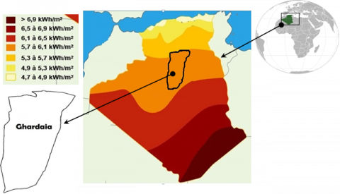
The study area covers the province of Ghardaa (32.2° - 32.82° N, and 3.7° and 4.5° E), which is located in the desert region of Algeria (Figure 1), and at an altitude of 450m. Rainfall during the year is low in Ghardaia, it is classified as BWh climat [15]. In Ghardaia. The average precipitation is 68 mm, the average annual temperature is 21.0℃. The city has great solar potential throughout the year due to its location (the average daily solar radiation received is approximately 6000 Wh.m2) on a horizontal surface. The data sets used for this study include the total daily solar radiation on a horizontal surface measured and recorded at the Applied Research Unit for Renewable Energies URAER for the four-year period from January 1 (2013) to December 31 (2016). The first three years set of 2013-2015 was used as the training data set while the last year (2016) is used to test the different models.
2.2 Refinement of data
The accuracy of the models is greatly affected by the quality of the data used. It is preferable to perform the data cleaning procedure for improving the quality of the data by filtering it from any error or doubt.
The dataset of the daily solar radiation used includes unreliable values [16]. Therefore, we carried out a procedure in this work to filter the raw data before the design of the daily GSR.
1. For the knowledge of the inaccurate daily SR values, the daily clearness index K is calculated, the values which are outside the range 0.015 < K < 1 have been deleted [17].
2. A month is deleted from the dataset, if the incorrect values are greater than five days in this month; if the number is less than five, the values are replaced by correct values based on the interpolation [18]. Due to certain atmospheric phenomena such as cloud extinction and aerosol extinction that occur when solar radiation travels through the atmosphere, all values of H must be less than H0 in the data available, which means K < 1.
In Table 1, the variables used as inputs are very appropriate, where the close agreement is between Tmin, Tmax, Tmean, H0 and solar radiation. The lowest value of solar radiation is recorded during the month of December and the highest value is recorded in the month of July. In terms of relative humidity, this is the opposite of solar radiation, where the highest value is recorded during the month of July and the lowest value in the month of December.
The minimum temperature data and the minimum, medium and maximum humidity data are positively skewed with the average skewness factors of 0.02, 0.37, 0.24, 0.43 respectively, while the maximum and medium temperature data and extraterrestrial solar radiation, and daily incident solar radiation are negatively skewed with the average skewness factors of -0.04, -0.02, -0.24, -0.15, as expected.
Figure 1. The study area site
Table 1. The climatological cycle of daily global solar radiation for the study period
|
Inputs data |
Min |
Max |
Mea |
Std |
Ske |
Kur |
r |
|
|
Train |
Tmin |
1.20 |
34.90 |
17.15 |
8.01 |
0.001 |
1.78 |
0.63 |
|
Tmax |
10.70 |
47.30 |
29.43 |
9.11 |
-0.070 |
1.79 |
0.69 |
|
|
Tmean |
1.20 |
34.90 |
21.15 |
8.01 |
0.001 |
1.78 |
0.63 |
|
|
RHmin |
18.26 |
51.02 |
21.15 |
10.80 |
0.442 |
2.76 |
-0.66 |
|
|
RHmean |
18.25 |
97.50 |
49.94 |
17.86 |
0.323 |
2.32 |
-0.65 |
|
|
H0 |
18.25 |
41.43 |
31.40 |
8.05 |
-0.271 |
1.59 |
0.90 |
|
|
H |
9.26 |
30.81 |
20.84 |
5.79 |
-0.060 |
1.68 |
1 |
|
|
Test |
Tmin |
3.03 |
33.70 |
17.28 |
7.84 |
0.070 |
1.69 |
0.69 |
|
Tmax |
11.80 |
45.80 |
29.25 |
8.90 |
0.016 |
1.69 |
0.74 |
|
|
Tmean |
7.20 |
38.90 |
23.01 |
8.49 |
0.046 |
1.67 |
0.73 |
|
|
RHmin |
0.50 |
57.02 |
22.69 |
11.32 |
0.472 |
2.98 |
-0.71 |
|
|
RHmean |
18.20 |
95.50 |
50.02 |
17.82 |
0.323 |
2.41 |
-0.70 |
|
|
H0 |
30.91 |
41.43 |
18.25 |
8.26 |
-0.205 |
1.53 |
0.94 |
|
|
H |
9.20 |
29.96 |
20.72 |
5.95 |
-0.116 |
1.65 |
1 |
|
Statistically, two numerical measures of shape (skewness and excess kurtosis) can be used to test for normality. For kurtosis, the general guideline is that if the number is greater than +1, the distribution is peaked. If skewness is not close to zero, then your data set is not Gaussian distributed [19] as expected, all the data can be considered as Gaussian in their distributional behaviors. All the data can be considered as Gaussian in their distributional behaviors (Table 1).
2.3 Gaussian process regression (GPR)
GPR is a non-parametric model based on the Gaussian probability distribution [20]; it can be defined as a collection of random variables, of which any finite number GP has a joint Gaussian distribution [21]. Thus, a GP is completely specified by its 2nd order statistics,
$f(x) \sim G P\left(m(x), k\left(x, x^{\prime}\right)\right)$ (1)
where, m(x) and $k\left(x, x^{\prime}\right)$ are the mean and covariance function of a real process f(x) respectively.
Suppose that a training set $\left\{\left(x_{i}, y_{i}\right), i=1 \ldots \ldots n\right\}$ The relationship between the $p-$ dimensional predictor $x \in \mathbb{R}^{p}$ and the target variable y is expressed as:
$y=f(x)+\varepsilon$ (2)
where, $\varepsilon$ is assumed to be an additive idd Gaussian noise, $\varepsilon \sim \mathrm{N}\left(0, \sigma_{n}^{2}\right)$.
The prior on the noisy observation becomes:
$\operatorname{cov}(y)=K(X, X)+\sigma_{n}^{2} I$ (3)
where, I denote the identy matrix of size n.
The joint distribution of the observed target values and the function values at the test locations prior is given by:
$\left|\begin{array}{l}
y \\
f_{*}
\end{array}\right| \sim \mathrm{N}\left(0 .\left|\begin{array}{cc}
K(X, X)+\sigma_{n}^{2} & K\left(X_{*}, X\right) \\
K\left(X_{*}, X\right) & K\left(X_{*}, X_{*}\right)
\end{array}\right|\right)$ (4)
where, $K\left(X, X_{*}\right)_{n \times n_{*}}$ denotes the covariance (or Gram) matrix between training test and also for different matrix $K\left(X_{*}, X\right), K\left(X_{*}, X_{*}\right) \operatorname{and} K(X, X) .$
The predictive equations for GPR becomes [22].
$f_{*} \mid X, y, X_{*} \sim \mathrm{N}\left(\bar{f}_{*}, \operatorname{cov}\left(f_{*}\right)\right)$ (5)
where,
$\operatorname{cov}\left(f_{*}=K\left(X_{*}, X_{*}\right)-\bar{f}_{*} K\left(X, X_{*}\right)\right.$ (6)
for a single test point $X_{*}$, the predictive distribution is a Gaussian distribution with mean and covariance given by:
$f_{*}=k_{*}^{T}\left(K+\sigma_{n}^{2} I\right)^{-1} y$ (7)
$\mathbb{V}\left[f_{*}\right]=k\left(x_{*}, x_{*}\right)-\bar{f}_{*} k_{*}$ (8)
where: $K=K(X, X), K_{*}=K\left(X, X_{*}\right) \text { and } k\left(x_{*}\right)=k_{*}$ denote the vector of covariances between the test point and the n training points. In the Eqns. (8) and (9), $\left(K+\sigma_{n}^{2} I\right)^{-1}$ can be calculated using Cholesky factorization [23].
2.4 Wavelet decomposition
The main motivation for using wavelet decomposition (WD) is the simple analysis of the series obtained. For many years, WD (or Wavelet transform) has been mixed with time series models as a preprocessing technique. WD uses a set of filters to decompose the original time series iteratively, so that separate forecasting models can be applied to each component.
The continuous wavelet transform (CWT) of a function f(t), compared to the mother wavelet $\psi(t)$ can be written by the following integral [24]:
$F_{w}(a, \tau)=|a|^{-\frac{1}{2}} \int_{-\infty}^{+\infty} f(t) \psi^{*}\left(\frac{1-\tau}{a}\right) d t$ (9)
where, (*) represents the operation of the complex conjugation, $\tau \in \mathbb{R}$ is the translational value and $a \in \mathbb{R}^{+*}$ is the scaling coefficient. Unlike the Fourier transformation, the CWT has been discretized and is known as the discrete wavelet transform (DWT).
The approach is an implementation of the wavelet transform by scaling and translation of the wavelets in discrete time. In this case, the wavelets are given by:
$\psi_{n, k}(t)=\left|a_{0}^{n}\right|^{-\frac{1}{2}} \psi\left(\frac{1-k \tau_{0} a_{0}^{n}}{a_{0}^{n}}\right)$ (10)
where, n and k are integers and $a=a_{0}^{n}, \tau=k \tau_{0} a_{0}^{n}$.
More details on Wavelet transform can be found in the literature [24] and [25].
2.5 Structure of the hybrid model
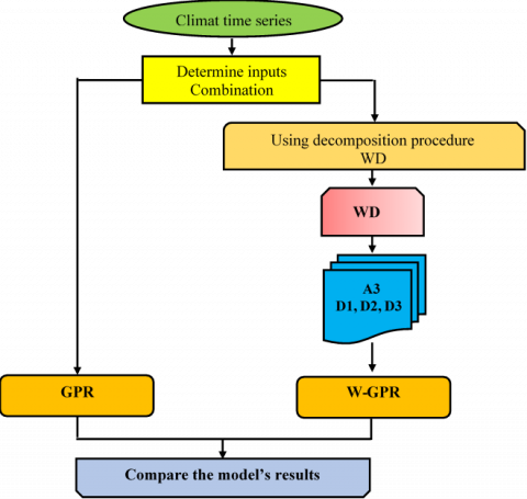
We use W-GPR to predict daily solar radiation in the desert region. Through this study, we used wavelet analysis to decompose the time series of meteorological data into different components. The optimal GPR parameters are represented in the flow chart of Figure 2 based on the wavelet transform algorithm.
Figure 2. The flow chart of the proposed model of the wavelet-Gaussian process regression W-GPR
2.6 Model input data
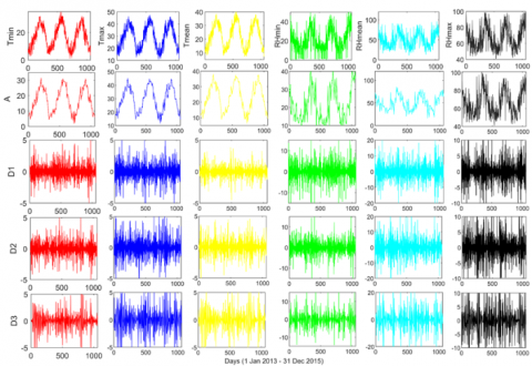
Figure 3 shows the DWCs of the seven input variables using coiflet type wavelets (Table 2) with three levels of detailed decompositions and one level of approximation, where the approximate level has the lowest frequency. Many works use the entire wavelet sub-series [26], while other works delete the detail component and keep the remaining sub-series as noise based on the correlation coefficient [27].
In the proposed approach, we consider each wavelet-decomposed signal in its original form to capture their random attributes and their physical structure; on this basis, we insert the entire substring into the W-GPR model.
Figure 3. DWC of the inputs of the W-GPR model from 01-Jan-2013 to 31-December-2015 for Ghardaia Aero
Table 2. Effect of the wavelet type on model accuracy
|
|
R2 |
MAE |
MSE |
RMSE |
|
db4 |
0.93 |
1.72 |
6.28 |
2.02 |
|
db8 |
0.94 |
1.30 |
5.89 |
1. 74 |
|
sym2 |
0.94 |
1.33 |
7.14 |
2.32 |
|
Sym8 |
0.94 |
1.27 |
5.71 |
1.89 |
|
coif1 |
0.96 |
1.02 |
5.25 |
1.81 |
|
coif3 |
0.95 |
1.14 |
5.34 |
1.83 |
|
coif5 |
0.93 |
2.93 |
17.31 |
3.66 |
|
dmey |
0.94 |
1.41 |
5.31 |
1.83 |
2.7 Performance evaluation
The performance of the proposed models (W-GPR) are tested based on the following statistical measures:
$r^{2}=\frac{\left(\sum_{n=1}^{n}\left(H_{n, O b s}-\bar{H}_{n, \text { obs }}\right)\left(H_{n, \text { Pred }}-\bar{H}_{n, \text { Pred }}\right)\right)^{2}}{\sum_{i=1}^{N}\left(H_{n, O b s}-\bar{H}_{n, o b s}\right)^{2} \sum_{n=1}^{n}\left(H_{n, \text { Pred }}-\bar{H}_{n, \text { Pred }}\right)^{2}}$ (11)
$\mathrm{RMSE}=\sqrt{\frac{\sum_{\mathrm{n}=1}^{\mathrm{n}}\left(\mathrm{H}_{\mathrm{n}, \mathrm{Obs}}-\mathrm{H}_{\mathrm{n}, \mathrm{Pred})^{2}}\right.}{\mathrm{N}}}$ (12)
$\mathrm{MAE}=\frac{1}{\mathrm{~N}} \sum_{\mathrm{i}=1}^{\mathrm{N}}\left|\left(\mathrm{H}_{\mathrm{n}, \text { Pred }}-\mathrm{H}_{\mathrm{n}, \mathrm{Obs}}\right)\right|$ (13)
where,
Hi,Obs :observed values
Hn,Pred: predicted values
$\bar{H}$n,obs: mean value of observations.
$\bar{H}$n,pred: mean value of predictions.
N: total number of data.
r2: Coefficient of determination.
RMSE: Root Mean Square Error.
MAE: Mean Absolute Error.
rRMSE: relative Root Mean Square Error.
According to Paul et al. [28] the performance of the model by considering the rRMSE is defined as:
rRMS E < 10 % the performance is Excellent.
10 % < rRMS E < 20 % the performance is Good.
20 % < rRMS E < 30 % the performance is Fair.
rRMS E > 30 % the performance is Poor.
3.1 Effect of wavelet type
Because of the importance of choosing the type of wavelets to decompose the variable input into details and approximation components in the precision of the models [29, 30], Table 2 presented the results of the application of eight mother wavelet, the highest precision concerns coif1 (Coiflet) (RMSE = 1.81 MJ/ m2Day).
In this paper, extraterrestrial solar radiation H0 was used as the primary predictor variable, and then the input combinations were divided into three groups:
$\begin{array}{l}
W-G P R 1: \\
(\mathrm{M} 1=[\mathrm{H} 0, \mathrm{Tmax}] \\
\mathrm{M} 2=[\mathrm{H} 0, \operatorname{Tmax}, \mathrm{Tmin}] \\
\mathrm{M} 3=[\mathrm{H} 0, \text { Tmax, } \text { Tmin, Tmean }]
\end{array}$
$\begin{array}{l}
W-G P R 2: \\
(\mathrm{M} 4=[\mathrm{H} 0, \mathrm{RHmean}] \\
\mathrm{M} 5=[\mathrm{H} 0, \mathrm{RHmean}, \mathrm{RHmin}] \\
\mathrm{M} 6=[\mathrm{H} 0, \mathrm{RHmean}, \mathrm{RHmin}, \mathrm{RHmax}]
\end{array}$
$\begin{array}{l}
W-\text { GPR3 : } \\
\text { (M7 = [H0, Tmax, RHmean, Tmin, RHmin] } \\
\text { M8 = [H0, Tmax, RHmean, Tmin, RHmin, Tmean] } \\
\text { M9= [H0, Tmax, RHmean, Tmin, RHmin, RHmax] } \\
\text { M10 = [All predictors variables] }
\end{array}$
Careful examination of Table 3 shows that the best performance that can be obtained is to include all inputs except the Tmean (M2) for the first group (W-GPR1), with R2 = 0.95 and, rRMSE = 11.76 % compared to R2= 0.95 and rRMSE = 12.10% (M3). For the second group (W-GPR2) the performance is better in (M4) with R2= 0.94 and rRMSE = 12.59% compared to R2= 0.94, rRMSE = 12.80% (M5), for (W-GPR3) the performance of the model is best in (M9) verified by R2 = 0.96 and rRMSE = 11.21 % in (M9) compared to R2= 0.96, rRMSE = 11.34 % in (M10).
By comparing the forecasts of the three models, the third group (W-GPR3) exceeds the expectations of the other models. The correlation coefficient not only records the highest values (0.96) compared to (0.95) for GPR3, (0.913) for W-GPR1 and (0.95) for W-GPR2, but also marks the lowest value of rRMSE (11.21%) compared to (12.52 %) for the classic model.
Table 3. Effect of the wavelet type on model accuracy
|
Input combinations |
Wavelet-coupled (W-GPR) model |
Classical (non-wavelet) GPR model |
||||||||
|
R2 |
MAE |
MSE |
RMSE |
rRMSE |
R2 |
MAE |
MSE |
RMSE |
rRMSE |
|
|
M1[H0, Tmax] |
0.94 |
1.24 |
7.16 |
2.18 |
12.40 |
0.94 |
1.4 |
7.91 |
2.4 |
13.69 |
|
M2[H0, Tmax,Tmin] |
0.95 |
1.06 |
5.81 |
1.93 |
11.76 |
0.94 |
1.29 |
7 |
2.23 |
12.87 |
|
M3 [H0, Tmax,Tmin, Tmean] |
0.95 |
1.11 |
6.17 |
2.00 |
12.10 |
0.94 |
1.31 |
7.22 |
2.27 |
13.06 |
|
M4 [H0, RHmean] |
0.94 |
1.20 |
6.50 |
2.10 |
12.59 |
0.94 |
1.34 |
7.13 |
2.26 |
12.99 |
|
M5 [H0, RHmean,RHmin] |
0.94 |
1.20 |
6.93 |
2.14 |
12.80 |
0.94 |
1.35 |
7.07 |
2.25 |
12.93 |
|
M6 [H0, RHmean,RHmin, RHmax] |
0.94 |
1.19 |
6.58 |
2.11 |
12.66 |
0.94 |
1.3 |
6.79 |
2.2 |
12.68 |
|
M7 [H0, Tmax, RHmean, Tmin, RHmin] |
0.95 |
1.07 |
5.51 |
1.91 |
11.67 |
0.95 |
1.25 |
6.80 |
2.2 |
12.69 |
|
M8 [H0, Tmax, RHmean, Tmin, RHmin, Tmean] |
0.95 |
1.09 |
5.89 |
1.94 |
11.84 |
0.95 |
1.26 |
6.84 |
2.21 |
12.73 |
|
M9 [H0, Tmax, RHmean, Tmin, RHmin, RHmax] |
0.96 |
1.02 |
5.25 |
1.81 |
11.21 |
0.95 |
1.22 |
6.38 |
2.12 |
12.31 |
|
M10 [All] |
0.96 |
1.04 |
5.38 |
1.84 |
11.34 |
0.95 |
1.24 |
6.61 |
2.16 |
12.52 |
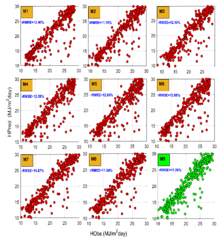
The ideal value of R2 is one, which means a perfect match between predicted and measured values. The scatterplot of the predicted value Hn,pred and the measured Hn,obs are shown in Figure 4, the model M9 is considered to be the optimal combination (R2 = 0.96).
Figure 4. Scatterplots of the regression value of solar radiation versus the measured, with different input combinations
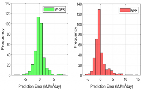
Visual representation of statistics has a big role in understanding the error range, to know the propagation of the error Pe, we use the histogram, based on this representation the prediction errors are large for the GPR model and although they are relatively less for W -GPR (M9) as shown in Figure 5. Which confirms the results obtained in Table 3.
Figure 6 shows the performance of the M9 model with W-GPR, GPR based on rRMSE measurement. W-GPR shows better performance than with the GPR model.
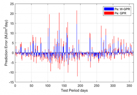
Figure 7 traces the prediction error (Pe = Hn,pred – Hn,obs). Input combinations of Table 2 are used. According to Table 3 and Figure 6, the comparison between the classical model and the W-GPR models shows that the use of the wavelet transform increases the precision of the model in the forecasts.
Figure 5. The spread of prediction error for (W-GPR) compared with GPR model
Figure 6. Comparison of the performance of the W-GPR with GPR
Figure 7. The prediction error in test period
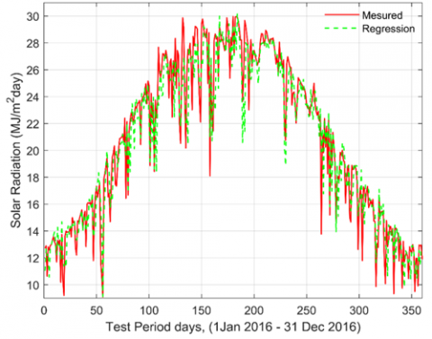
To better see the occurrence of large errors in forecasting, the predicted daily global solar radiation and observed values over the testing period (year 2016) are depicted in Figure 8. It is clearly illustrated that great changes of weather types of two consecutive days (sunny days to overcast days and overcast days to sunny days) result in large errors of forecasting.
Figure 8. Measured global radiation versus estimated best W-GPR model M9
In some cases, the model is not capable to predict values of solar radiation with accuracy. The reason behind this issue is that some events presented to the model in the validation phase are not similar to those used in the training process.
Since the prediction of solar radiation is very important in the management of solar systems. This paper investigated the possibility of prediction of W-GPR model, for daily solar radiation with high precision. Ten W-GPR models were developed using different combinations of inputs: Tmin, Tmax, RHmin, RHmax, RHmean and H0. In order to evaluate the models and test their accuracy on the prediction, we used five statistical indicators. The results showed the significant effect of the wavelet type on the precision of the W-GPR models, where the wavelet type coif1 (Coiflet) has the highest precision, and the combination H0, Tmin, Tmax, RHmin, RHmax, RHmean offers great precision compared to the other proposed W-GPR models. To demonstrate the accuracy of the W-GPR model, its predictions are compared to the classical model (GPR). The results showed a significant improvement in the performance of the W-GPR model appearing in the statistical indices R2 = 0.960, MAE=1.02 MJ/m2day, MSE=5.25 MJ/m2day, RMSE= 1.81 MJ/m2day, rRMSE= 11.21%. Finally, this model can be used to predict daily solar radiation in areas with a similar climate and can be further improved by introducing other variables, which should be the focus of our future work.
|
$H_{0}$ |
Extra-terrestrial solar radiation (MJ/m2 Day) |
|
$G_{S C}$ |
Solar constant (1367 W/m2) |
|
$\delta$ |
Solar declination (rad) |
|
$\omega_{s}$ |
Mean sunrise hour angle (rad) |
|
$\varphi$ |
Latitude of the region (rad) |
|
K |
Clearness index |
|
nday |
day number of the year |
|
$H_{n, O b s}$ |
observed values (MJ/m2 Day) |
|
$H_{n, \text { Pred }}$ |
predicted values (MJ/m2 Day) |
|
$\bar{H}_{n, O b s}$ |
Mean value of observations (MJ/m2 Day) |
|
$\bar{H}_{n, \text { Pred }}$ |
Mean value of predictions (MJ/m2 Day) |
|
MAE |
Mean Absolute bias Error (MJ/m2 Day) |
|
MSE |
Mean Square Error (MJ/m2 Day) |
|
RMSE |
Root Mean Square Error (MJ/m2 Day) |
|
rRMSE |
normalized Relative Mean Square Error (%) |
|
r |
Correlation Coefficient |
|
R2 |
Détermination Coefficient |
H0 as the extraterrestrial solar radiation is computed as [31]:
$\begin{aligned}
H_{0}=\frac{24 \times 3600}{\pi} G_{s c}\left(1+\frac{0.033 \cos \left(3600 \times n_{\text {day }}\right)}{365}\right)\left(\cos (\varphi) \sin \left(\omega_{s}\right)+\right.\\
&\left.\frac{\pi \omega_{s}}{180}\right) \sin (\varphi) \sin (\delta)
\end{aligned}$
where:
Gsc: Solar constant (1367 W/m2) [32].
$\varphi$: Latitude of the location.
nday: Day number of the year.
$\delta \text { and } \omega$: Daily solar declination and sunset hour angle, respectively calculated by:
$\delta=\frac{23.45 \pi}{180} \sin \left[\frac{360}{365}\left(n_{\text {day }}+284\right)\right]$ (3)
$\omega_{s}=\arccos [-\tan (\delta) \tan (\varphi)]$
Clearness Index (K): is a ratio of measured solar radiation in a locale relative to the extraterrestrial solar radiation.
[1] Majumder, I., Dash, P.K., Bisoi, R. (2019). Short-term solar power prediction using multi-kernel-based random vector functional link with water cycle algorithm-based parameter optimization. Neural Computing and Applications, 1-19. https://doi.org/10.1007/s00521-019-04290-x
[2] Fan, J., Wu, L., Zhang, F., Cai, H., Ma, X., Bai, H. (2019). Evaluation and development of empirical models for estimating daily and monthly mean daily diffuse horizontal solar radiation for different climatic regions of China. Renewable and Sustainable Energy Reviews, 105: 168-186. https://doi.org/10.1016/j.rser.2019.01.040
[3] Liu, J., Pan, T., Chen, D., Zhou, X., Yu, Q., Flerchinger, G.N., Shen, Y. (2017). An improved Ångström-type model for estimating solar radiation over the Tibetan Plateau. Energies, 10(7): 892. https://doi.org/10.3390/en10070892
[4] Belmahdi, B., Louzazni, M., El Bouardi, A. (2020). One month-ahead forecasting of mean daily global solar radiation using time series models. Optik, 219: 165207. https://doi.org/10.1016/j.ijleo.2020.165207.
[5] Alsharif, M.H., Younes, M.K., Kim, J. (2019). Time series ARIMA model for prediction of daily and monthly average global solar radiation: The case study of Seoul, South Korea. Symmetry, 11(2): 240. https://doi.org/10.3390/sym11020240
[6] Benghanem, M., Mellit, A. (2010). Radial basis function network-based prediction of global solar radiation data: application for sizing of a stand-alone photovoltaic system at al-Madinah, Saudi Arabia, Energy, 35(9): 3751-3762. https://doi.org/10.1016/j.energy.2010.05.024
[7] Åenkal, O., Kuleli, T. (2009). Estimation of solar radiation over turkey using artificial neural network and satellite data, Applied Energy, 86(7): 1222-1228. https://doi.org/10.1016/j.apenergy.2008.06.003
[8] Shamshirband, S., Mohammadi, K., Chen, H.L., Narayana Samy, G., Petkovi, D., Ma, C. (2015). Daily global solar radiation prediction from air temperatures using kernel extreme learning machine: A case study for Iran, Journal of Atmospheric and Solar-Terrestrial Physics, 134(Complete): 109-117. https://doi.org/10.1016/j.solener.2015.03.015
[9] Pasolli, L., Melgani, F., Blanzieri, E. (2010). Gaussian process regression for estimating chlorophyll concentration in subsurface waters from remote sensing data. IEEE Geoscience and Remote Sensing Letters, 7(3): 464-468. https://doi.org/10.1109/LGRS.2009.2039191
[10] L´azaro-Gredilla, M., Titsias, M. K., Verrelst, J., Camps-Valls, G. (2014). Retrieval of biophysical parameters with heteroscedastic gaussian processes. IEEE Geoscience and Remote Sensing Letters, 11(4): 838-842. https://doi.org/10.1109/LGRS.2013.2279695
[11] Salcedo-Sanz, S., Casanova-Mateo, C., Mu˜noz-Mar´ı, J., Camps-Valls, G. (2014). Prediction of daily global solar irradiation using temporal gaussian processes. IEEE Geoscience and Remote Sensing Letters, 11(11): 1936-1940. https://doi.org/10.1109/LGRS.2014.2314315
[12] Guermoui, M., Gairaa, K., Rabehi, A., Djafer, D., Benkaciali, S. (2018). Estimation of the daily global solar radiation based on the gaussian process regression methodology in the Saharan climate. The European Physical Journal Plus, 133: 211. https://doi.org/10.1140/epjp/i2018-12029-7
[13] Quej, V.H., Almorox, J., Arnaldo, J.A., Saito, L. (2017). ANFIS, SVM and ANN soft-computing techniques to estimate daily global solar radiation in a warm sub-humid environment. Journal of Atmospheric and Solar-Terrestrial Physics, 155: 62-70. https://doi.org/10.1016/j.jastp.2017.02.002
[14] Shamshirband, S., Mohammadi, K., Khorasanizadeh, H., Yee, L., Lee, M., Petkovi´c, D., Zalnezhad, E. (2016) Estimating the diffuse solar radiation using a coupled support vector machine–wavelet transform model. Renewable and Sustainable Energy Reviews, 56: 428-435. https://doi.org/10.1016/j.rser.2015.11.055
[15] https://fr.climate-data.org/afrique/algerie/ghardaia-1123/ (November 2020, date last accessed).
[16] Mohammadi, K., Shamshirband, S., Tong, C.W., Arif, M., Petkovi´c, D., Ch, S. (2015). A new hybrid support vector machine–wavelet transform approach for estimation of horizontal global solar radiation. Energy Conversion and Management, 92: 162-171. https://doi.org/10.1016/j.enconman.2014.12.050
[17] Yadav, A.P., Behera, L. (2014). Solar radiation forecasting using neural networks and wavelet transform. IFAC Proceedings Volumes, 47(1): 890-896. https://doi.org/10.1016/j.rser.2013.08.055
[18] Turrado, C.C., López, M.D.C.M., Lasheras, F.S., Gómez, B.A.R., Rollé, J.L.C., Juez, F.J.D.C. (2014). Missing data imputation of solar radiation data under different atmospheric conditions. Sensors, 14(11): 20382-20399. https://doi.org/10.3390/s141120382
[19] George D, Paul, M. (2010). SPSS for Windows Step by Step: A Simple Guide and Reference, 17.0 Update. 10th ed. Boston: Allyn & Bacon.
[20] Roushangar, K., Shahnazi, S. (2020). Prediction of sediment transport rates in gravel-bed Rivers using Gaussian process regression. Journal of Hydroinformatics, 22(2): 249-262. https://doi.org/10.2166/hydro.2019.077
[21] Benavoli, A., Azzimonti, D., Piga, D. (2020). Skew Gaussian processes for classification. Machine Learning, 109(9): 1877-1902. https://doi.org/10.1007/s10994-020-05906-3
[22] Guan, Y.B. (2020). Introduction to gaussian processes for regression. Doctoral Dissertation, California State Polytechnic University, Pomona.
[23] Phoon, K.K., Huang, H.W., Quek, S.T. (2004). Comparison between Karhunen–Loeve and wavelet expansions for simulation of Gaussian processes. Computers & Structures, 82(13-14): 985-991. https://doi.org/10.1016/j.compstruc.2004.03.008
[24] Corradi, G., Sinou, J.J., Besset, S. (2020). Prediction of squeal noise based on multiresolution signal decomposition and wavelet representation-Application to FEM brake systems subjected to friction-induced vibration. Applied Sciences, 10(21): 7418. https://doi.org/10.3390/app10217418
[25] Daubechies, I. (1992). Ten lectures on wavelets. Society for Industrial and Applied Mathematics. https://doi.org/10.1137/1.9781611970104
[26] Zhang, D. (2019). Wavelet Transform. In Fundamentals of Image Data Mining, Springer, Cham, 35-44.
[27] Zhou, F., Liu, B., Duan, K. (2020). Coupling wavelet transform and artificial neural network for forecasting estuarine salinity. Journal of Hydrology, 588: 125127. https://doi.org/10.1016/j.jhydrol.2020.125127
[28] Paul, R.K., Paul, A.K., Bhar, L.M. (2020). Wavelet-based combination approach for modeling sub-divisional rainfall in India. Theoretical and Applied Climatology, 139(3): 949-963. https://doi.org/10.1007/s00704-019-03026-0
[29] Mihoub, R., Chabour, N., Guermoui, M. (2016). Modeling soil temperature based on gaussian process regression in a semi-arid-climate, case study ghardaia, Algeria. Geomechanics and Geophysics for Geo-Energy and Geo-Resources, 2(4): 397-403. https://doi.org/10.1007/s40948-016-0033-3
[30] Kulesza, K. (2020). Spatiotemporal variability and trends in global solar radiation over Poland based on satellite-derived data (1986–2015). International Journal of Climatology, 40(15): 6526-6543. https://doi.org/10.1002/joc.6596
[31] Rabehi, A., Guermoui, M., Lalmi, D. (2020). Hybrid models for global solar radiation prediction: A case study. International Journal of Ambient Energy, 41(1): 31-40. https://doi.org/10.1080/01430750.2018.1443498
[32] Fedorov, V.M. (2012). Interannual variability of the solar constant. Solar System Research, 46(2): 170-176. https://doi.org/10.1134/S0038094612020049